
Leakage Vortex Progression through a Guide Vane’s Clearance Gap and the Resulting Pressure Fluctuation in a Francis Turbine

 , ,
, ,  and
and
Abstract
:1. Introduction
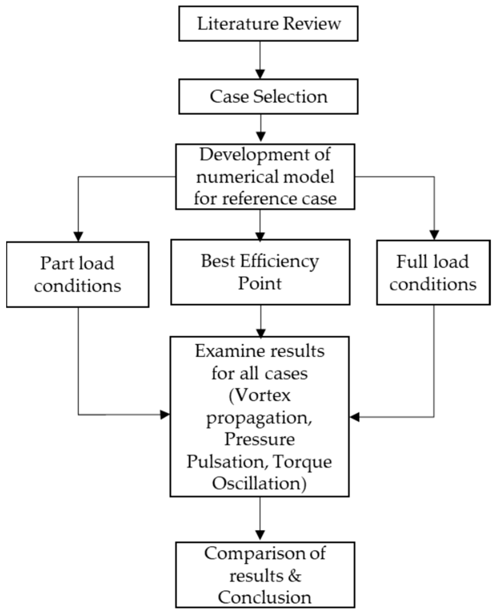
2. Methodology
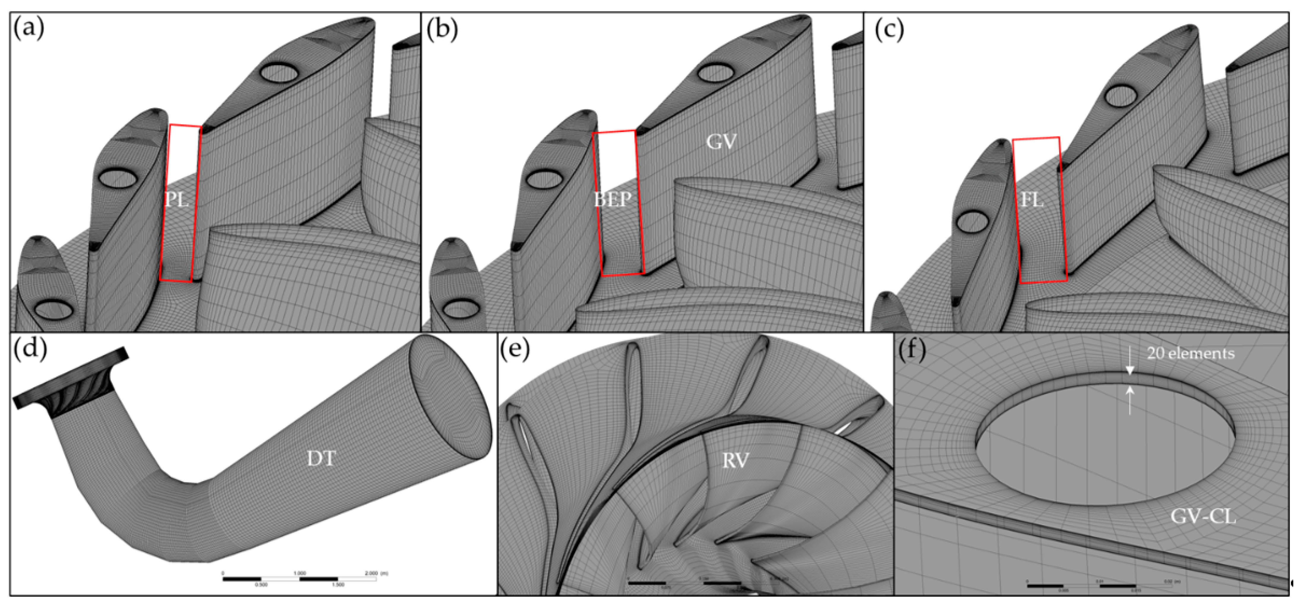
2.1. Mesh Generation and Boundary Conditions
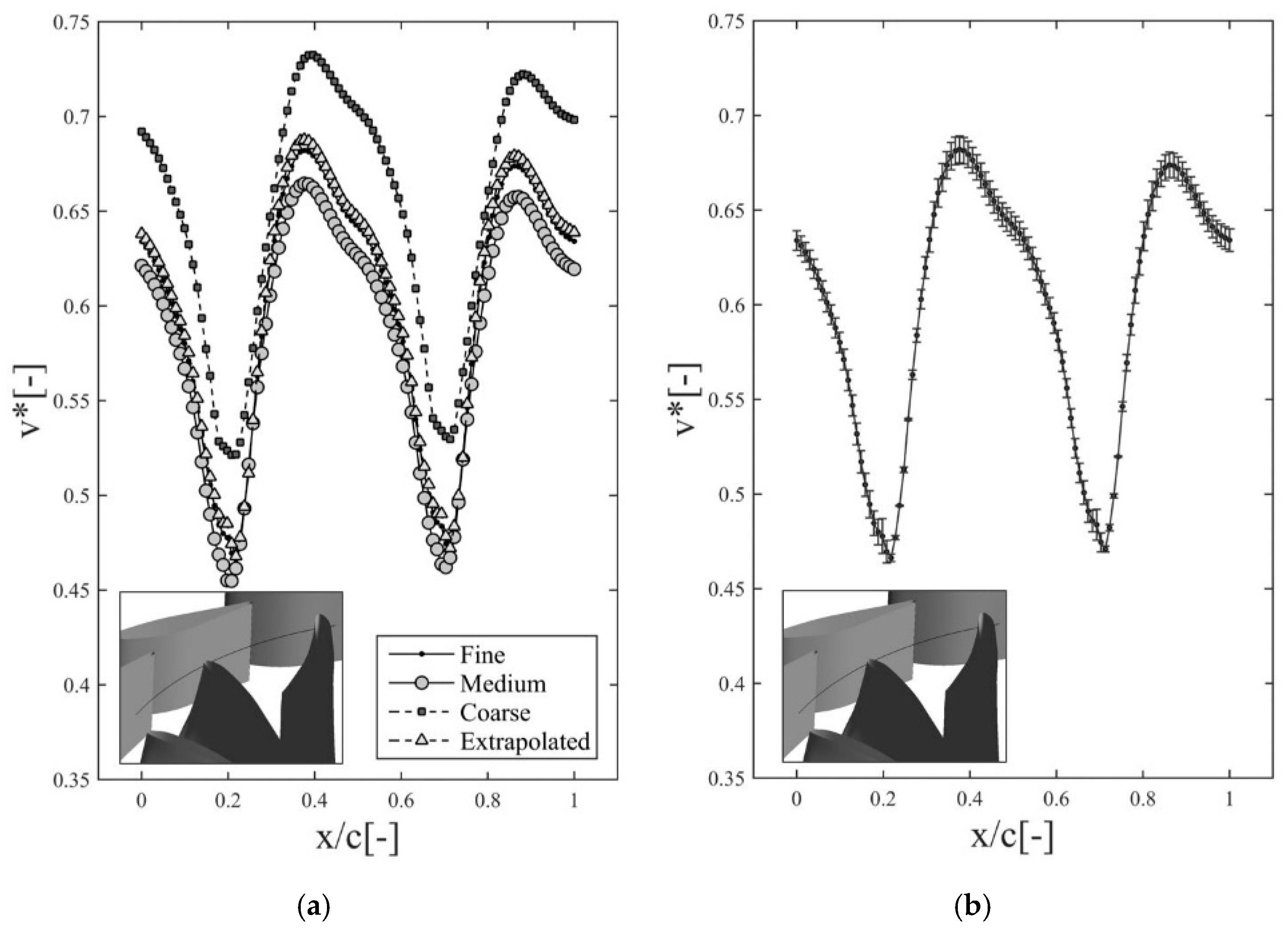
2.2. Mesh Sensitivity Analysis
- (i)
- Average length of each element for a 3D mesh was determined as follows:
- (ii)
- Let and . The apparent order was solved as in Equations (2)–(4) using a fixed point iteration method:
- (iii)
- The extrapolated values were calculated as follows:
- (iv)
- The approximate and extrapolated relative errors were calculated as follows:
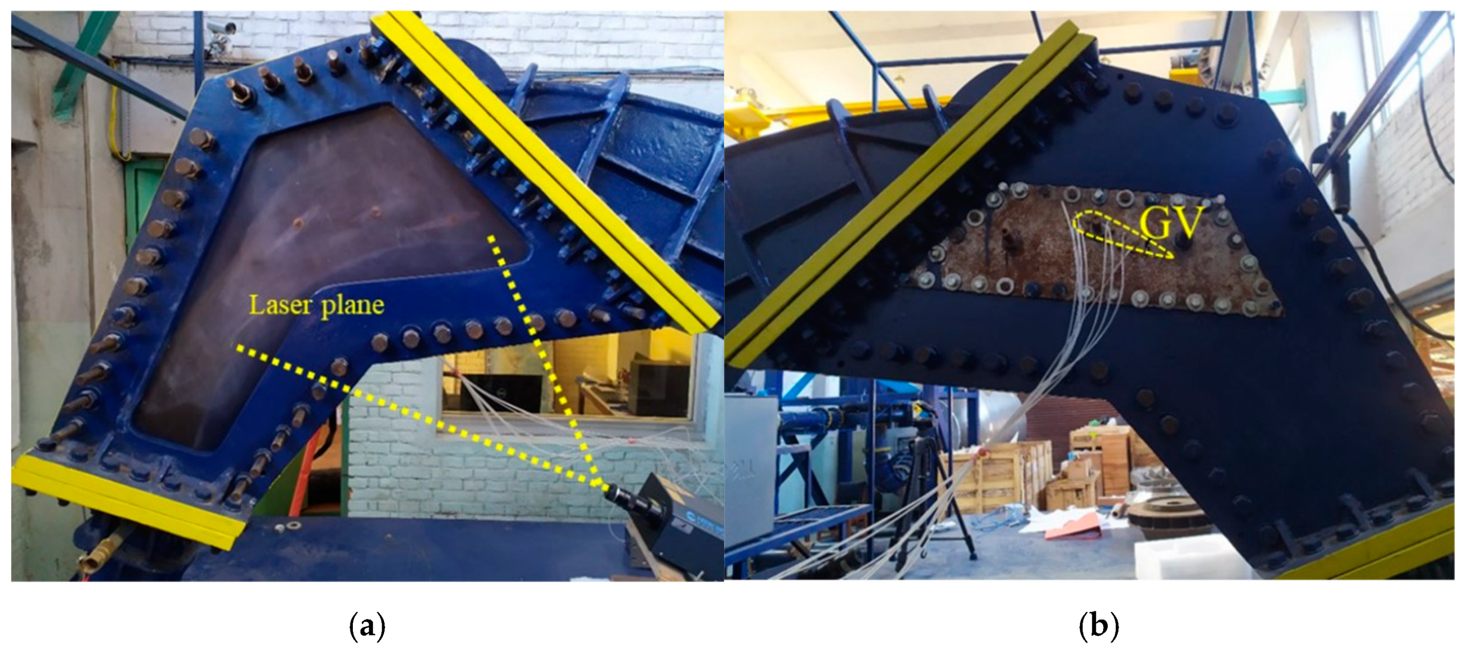
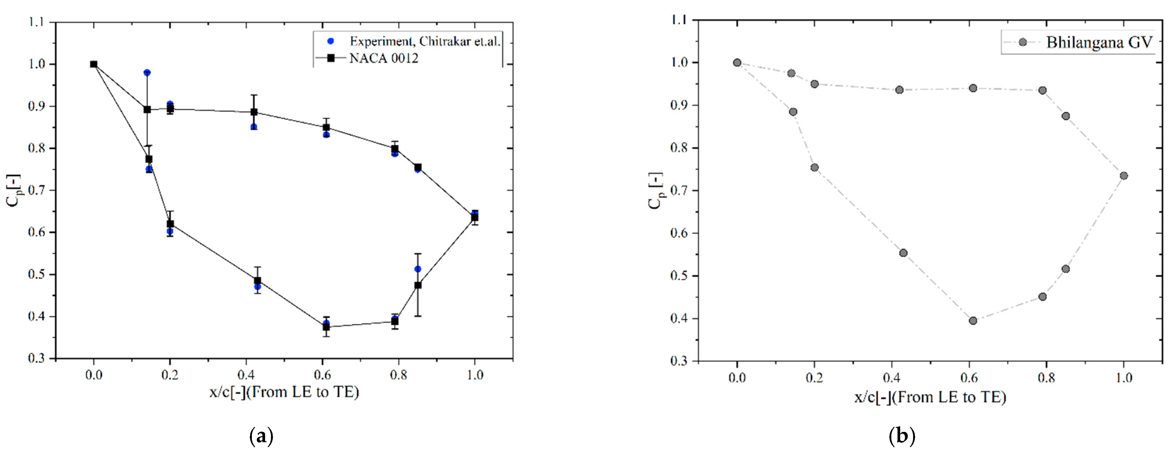
2.3. Validation with Prototype Data
3. Results and Discussions
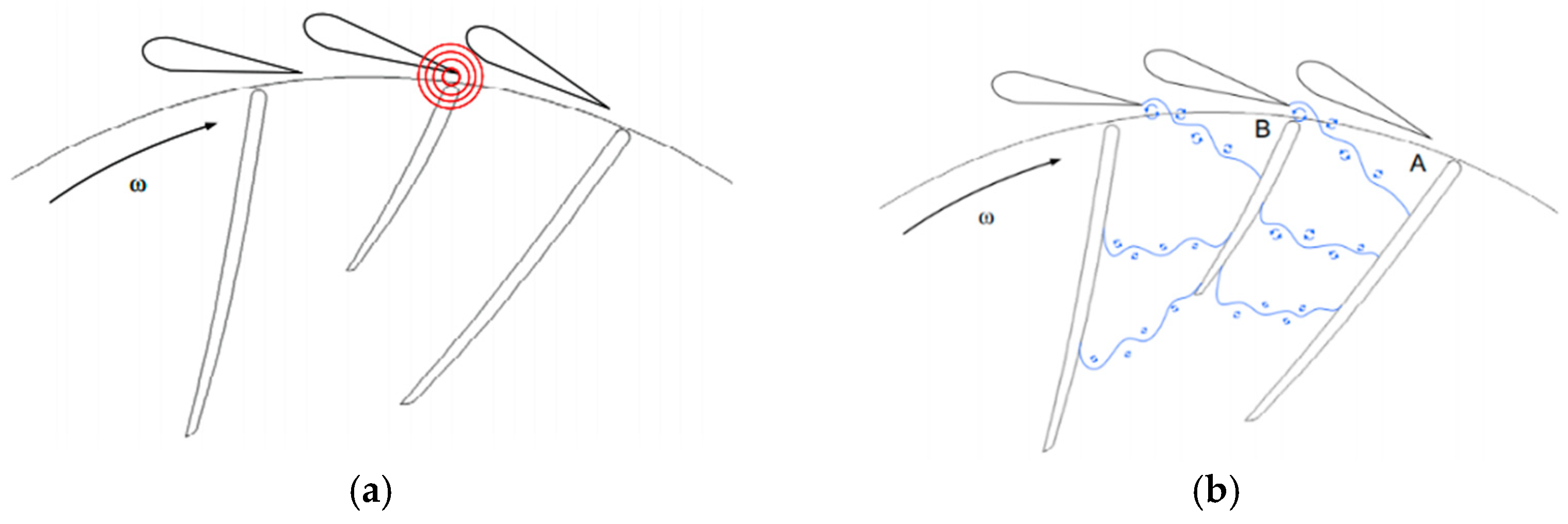
3.1. Leakage Vortex from GV
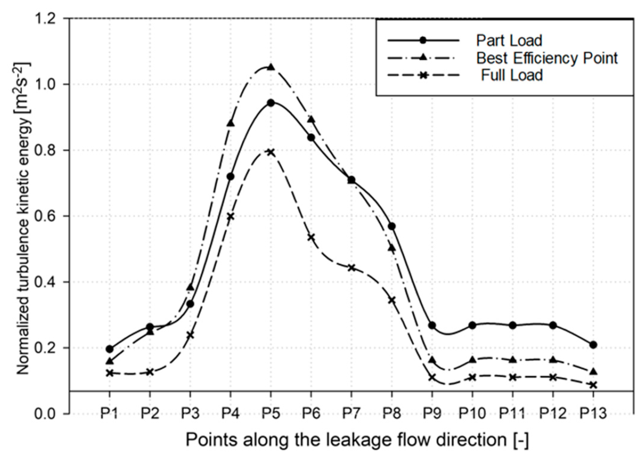
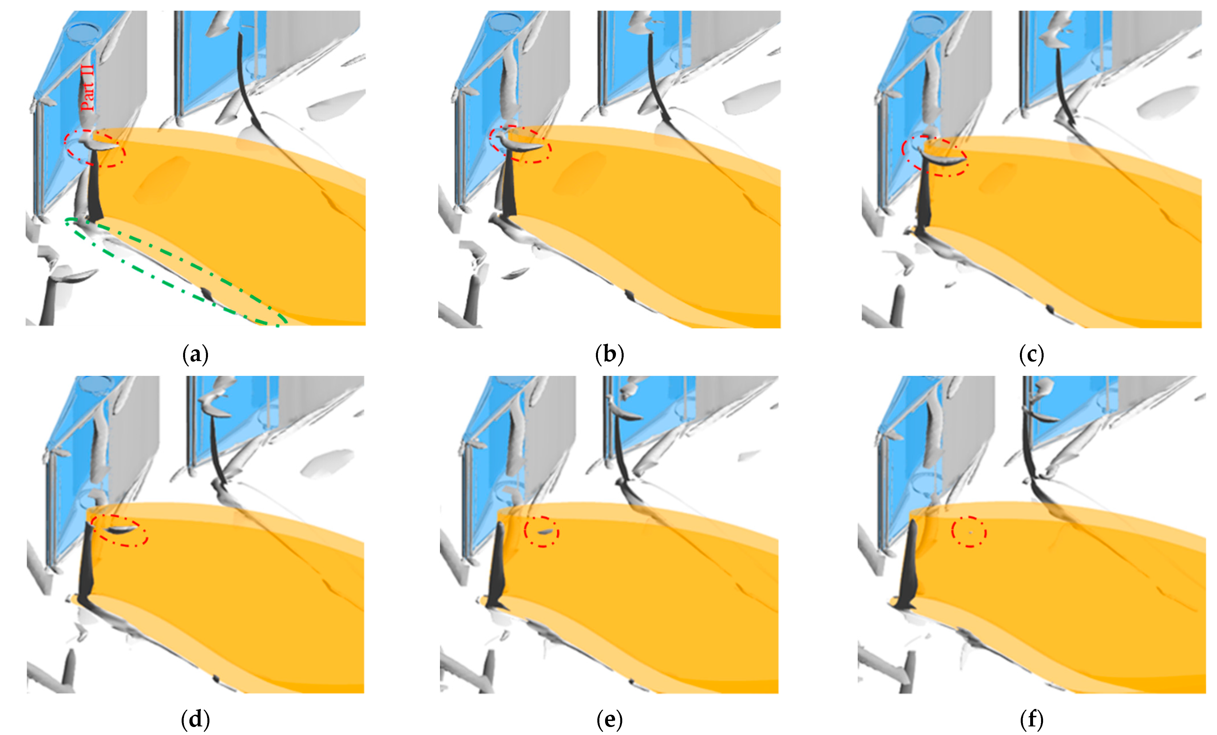
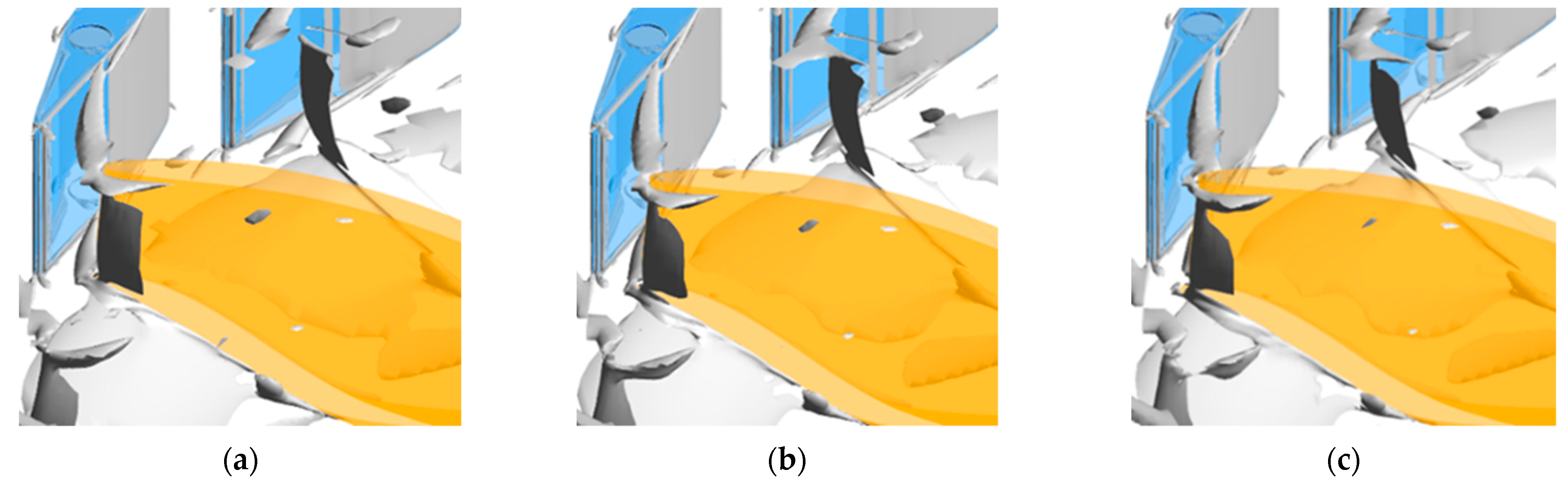
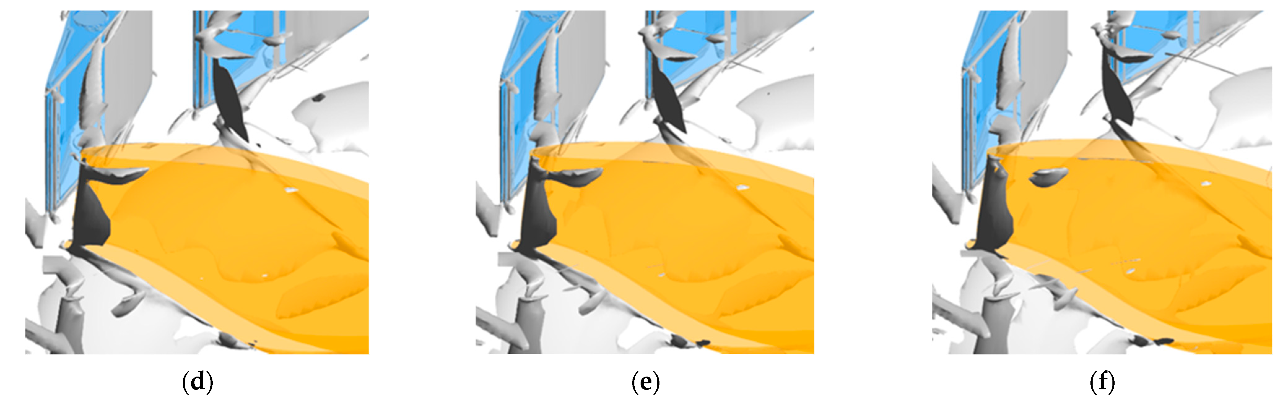
3.2. Leakage Vortex Progression
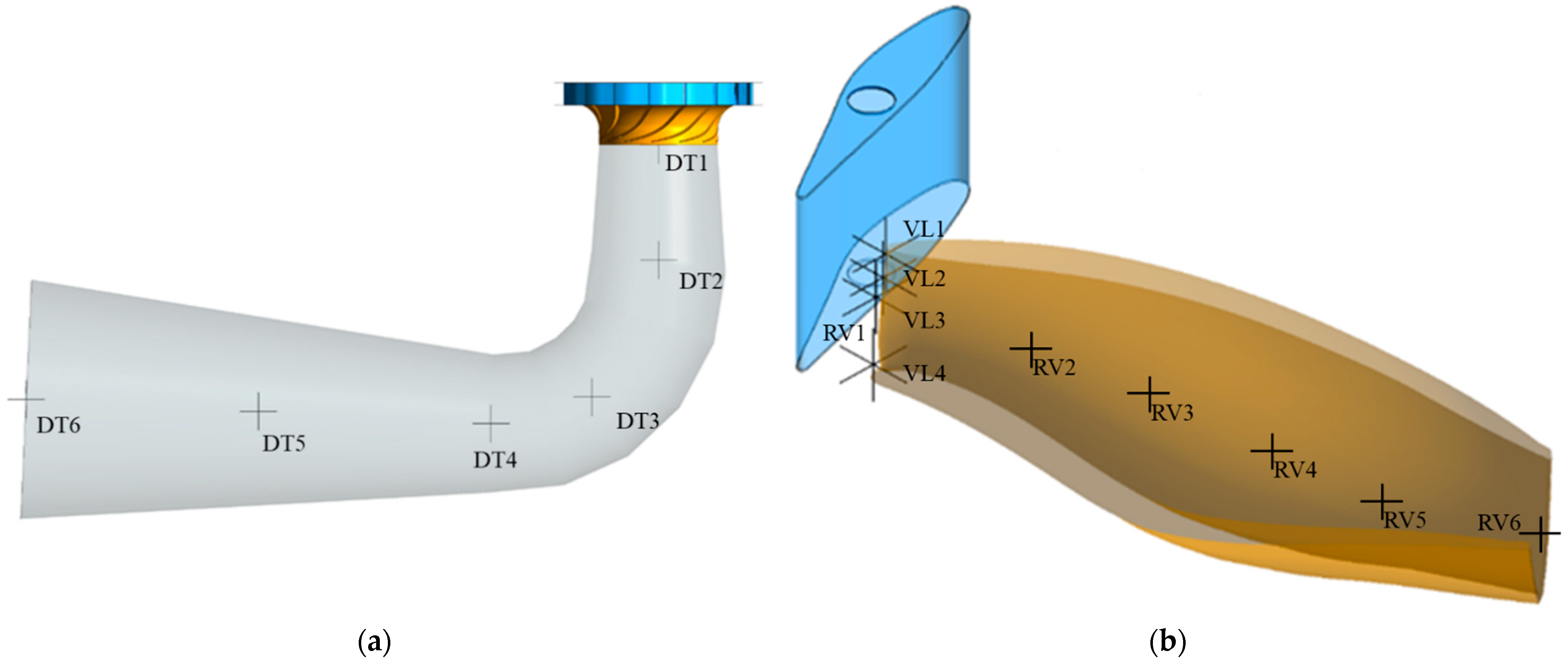
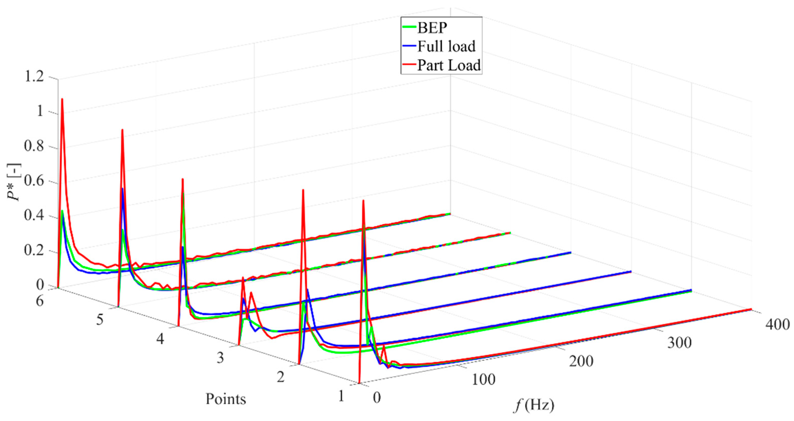
3.3. Pressure Pulsations Inside Runner
3.4. Torque Oscillations
4. Conclusions
Author Contributions
Funding
Data Availability Statement
Acknowledgments
Conflicts of Interest
Nomenclature
| GCIfine | Grid convergence index of the fine mesh [-] |
| ea | Approximate relative error [-] |
| eext | Extrapolated relative error [-] |
| fb | Blade passing Frequency [Hz] |
| f | Frequency [Hz] |
| H | Head [m] |
| n | Rotation of the runner [rpm] |
| Ph | Power [kW] |
| P* | Normalized Pressure [-] |
| Th | Hydraulic torque [Nm] |
| Tavg | Average torque [Nm] |
| Angular velocity [rads−1] | |
| Φ | Variable for GCI calculation [-] |
| v* | Normalized velocity [-] |
| v | Local velocity [ms−1] |
| Cp | Normalized pressure [-] |
| ρ | Density [kgm−3] |
| E | Specific hydraulic energy of turbine [J kg−1] |
| Zb | Number of rotating blades [-] |
| Zgv | Number of guide vanes [-] |
References
- Brekke, H. The influence from the Guide Vane Clearance Gap on Efficiency and Scale Effect for Francis Turbine. In Proceedings of the IAHR Symposium on Progress within Large and High Specific Energy Units, Trondheim, Norway, 20–23 June 1988; Volume 14, pp. 825–837. [Google Scholar]
- Thapa, B.S.; Dahlhaug, O.G.; Thapa, B. Sediment Erosion Induced Leakage Flow from Guide Vane Clearance Gap in a Low Specific Speed Francis Turbine. Renew. Energy 2017, 107, 253–261. [Google Scholar] [CrossRef]
- Chitrakar, S.; Thapa, B.S.; Dahlhaug, O.G.; Neopane, H.P. Numerical Investigation of the Flow Phenomena around a Low Specific Speed Francis Turbine’s Guide Vane Cascade. IOP Conf. Ser. Earth Environ. Sci. 2016, 49. [Google Scholar] [CrossRef] [Green Version]
- Koirala, R.; Thapa, B.; Neopane, H.P.; Zhu, B.; Chhetry, B. Sediment Erosion in Guide Vanes of Francis Turbine: A Case Study of Kaligandaki Hydropower Plant, Nepal. Wear 2016, 362–363, 53–60. [Google Scholar] [CrossRef]
- Koirala, R.; Zhu, B.; Neopane, H.P. Effect of Guide Vane Clearance Gap on Francis Turbine Performance. Energies 2016, 9, 275. [Google Scholar] [CrossRef]
- Liu, Y.; Han, Y.; Tan, L.; Wang, Y. Blade Rotation Angle on Energy Performance and Tip Leakage Vortex in a Mixed Flow Pump as Turbine at Pump Mode. Energy 2020, 206, 118084. [Google Scholar] [CrossRef]
- Chitrakar, S.; Dahlhaug, O.G.; Neopane, H.P. Numerical Investigation of the Effect of Leakage Flow through Erosion-Induced Clearance Gaps of Guide Vanes on the Performance of Francis Turbines. Eng. Appl. Comput. Fluid Mech. 2018, 12, 662–678. [Google Scholar] [CrossRef]
- Chitrakar, S.; Neopane, H.P.; Dahlhaug, O.G. Particle Image Velocimetry Investigation of the Leakage Flow through Clearance Gaps in Cambered Hydrofoils. J. Fluids Eng. Trans. ASME 2017, 139. [Google Scholar] [CrossRef]
- Gautam, S.; Neopane, H.P.; Thapa, B.S.; Chitrakar, S.; Zhu, B. Numerical Investigation of the Effects of Leakage Flow from Guide Vanes of Francis Turbines Using Alternative Clearance Gap Method. J. Appl. Fluid Mech. 2020, 13, 1407–1419. [Google Scholar] [CrossRef]
- Liu, Y.; Tan, L.; Wang, B. A Review of Tip Clearance in Propeller, Pump and Turbine. Energies 2018, 11, 2202. [Google Scholar] [CrossRef] [Green Version]
- Kobro, E. Measurement of Pressure Pulsations in Francis Turbines. Ph.D. Thesis, NTNU, Trondheim, Norway, 2010. [Google Scholar]
- Zhang, Y.; Liu, K.; Xian, H.; Du, X. A Review of Methods for Vortex Identification in Hydroturbines. Renew. Sustain. Energy Rev. 2018, 81, 1269–1285. [Google Scholar] [CrossRef]
- Qian, R. Flow Field Measurements in a Stator of a Hydraulic turbine. Ph.D. Thesis, Laval University, Quebec, QC, Canada, 2008. [Google Scholar]
- Chakraborty, P.; Balachandar, S.; Adrian, R.J. On the Relationships between Local Vortex Identification Schemes. J. Fluid Mech. 2005, 535, 189–214. [Google Scholar] [CrossRef] [Green Version]
- Elsas, J.H.; Moriconi, L. Vortex Identification from Local Properties of the Vorticity Field. Phys. Fluids 2017, 29. [Google Scholar] [CrossRef] [Green Version]
- ANSYS Inc. ANSYS Inc. ANSYS CFD-Post User’s Guide. In Vortex Core Region; ANSYS Inc: Canonsburg, PA, USA, 2017. [Google Scholar]
- Hunt, J.C.R.; Wray, A.A.; Eddies, P.M. Streams, and Convergence Zones in Turbulent Flows. In Center for Turbulence Research, Proceedings of the Summer Program; Stanford University: Stanford, CA, USA, 1988; pp. 193–208. [Google Scholar]
- Jeong, J.; Hussain, F. On the Identification of a Vortex. J. Fluid Mech. 1995, 69–94. [Google Scholar] [CrossRef]
- Chong, M.S.; Perry, A.E.; Cantwell, B.J. A General Classification of Three-Dimensional Flow Fields. Phys. Fluids A 1990, 2, 765–777. [Google Scholar] [CrossRef]
- Zhou, J.; Adrian, R.J.; Balachandar, S.; Kendall, T.M. Mechanisms for Generating Coherent Packets of Hairpin Vortices in Channel Flow. J. Fluid Mech. 1999, 387, 353–396. [Google Scholar] [CrossRef]
- Thapa, R.; Sharma, S.; Singh, K.M.; Gandhi, B.K. Numerical Investigation of Flow Field and Performance of the Francis Turbine of Bhilangana-III Hydropower Plant. J. Phys. Conf. Ser. 2020, 1608. [Google Scholar] [CrossRef]
- Acharya, N.; Trivedi, C.; Wahl, N.M.; Gautam, S.; Chitrakar, S.; Dahlhaug, O.G. Numerical Study of Sediment Erosion in Guide Vanes of a High Head Francis Turbine. J. Phys. Conf. Ser. 2019, 1266. [Google Scholar] [CrossRef] [Green Version]
- Gautam, S.; Neopane, H.P.; Acharya, N.; Chitrakar, S.; Thapa, B.S.; Zhu, B. Sediment Erosion in Low Specific Speed Francis Turbines: A Case Study on Effects and Causes. Wear 2020, 442–443. [Google Scholar] [CrossRef]
- IEC 60041: 1991–11; Field Acceptance Tests to Determine the Hydraulic Performance of Hydraulic Turbines, Storage Pumps and Pump-Turbines; International Electrotechnical Commission: Geneva, Switzerland, 1991.
- Trivedi, C.; Dahlhaug, O.G. A Comprehensive Review of Verification and Validation Techniques Applied to Hydraulic Turbines. Int. J. Fluid Mach. Syst. 2019, 12, 345–367. [Google Scholar] [CrossRef]
- Ansys Inc. CFX Solver Modelling Guide, Release 15.0. ANSYS CFX Solver Model. Guid. 2013, 15317, 724–746. [Google Scholar]
- Menter, F.R. Review of the Shear-Stress Transport Turbulence Model Experience from an Industrial Perspective. Int. J. Comut. Fluid Dyn. 2009, 23, 305–316. [Google Scholar] [CrossRef]
- Gautam, S.; Lama, R.; Chitrakar, S.; Thapa, B.S.; Zhu, B.; Neopane, H.P. Numerical Investigation on the Effects of Leakage Flow from Guide Vane-Clearance Gaps in Low Specific Speed Francis Turbines. J. Phys. Conf. Ser. 2020, 1608. [Google Scholar] [CrossRef]
- Trivedi, C.; Cervantes, M.J.; Dahlhaug, O.G. Numerical Techniques Applied to Hydraulic Turbines: A Perspective Review. Appl. Mech. Rev. 2016, 68, 1–18. [Google Scholar] [CrossRef]
- Arispe, T.M.; de Oliveira, W.; Ramirez, R.G. Francis Turbine Draft Tube Parameterization and Analysis of Performance Characteristics Using CFD Techniques. Renew. Energy 2018, 127, 114–124. [Google Scholar] [CrossRef]
- Celik, I.B.; Ghia, U.; Roache, P.J.; Freitas, C.J.; Coleman, H.; Raad, P.E. Procedure for Estimation and Reporting of Uncertainty Due to Discretization in CFD Applications. J. Fluids Eng. Trans. ASME 2008, 130, 0780011–0780014. [Google Scholar] [CrossRef] [Green Version]
- Trivedi, C.; Cervantes, M.J.; Gandhi, B.K.; Dahlhaug, O.G. Experimental and Numerical Studies for a High Head Francis Turbine at Several Operating Points. J. Fluids Eng. Trans. ASME 2013, 135, 1–17. [Google Scholar] [CrossRef]
- Shingai, K.; Okamoto, N.; Tamura, Y.; Tani, K. Long-Period Pressure Pulsation Estimated in Numerical Simulations for Excessive Flow Rate Condition of Francis Turbine. J. Fluids Eng. Trans. ASME 2014, 136, 1–9. [Google Scholar] [CrossRef]
- Chitrakar, S.; Neopane, H.P.; Dahlhaug, O.G. Development of a Test Rig for Investigating the Flow Field around Guide Vanes of Francis Turbines. Flow Meas. Instrum. 2019, 70, 101648. [Google Scholar] [CrossRef]
- Chitrakar, S.; Thapa, B.S.; Dahlhaug, O.G.; Neopane, H.P. Numerical and Experimental Study of the Leakage Flow in Guide Vanes with Different Hydrofoils. J. Comput. Des. Eng. 2017, 4, 218–230. [Google Scholar] [CrossRef]
- Trivedi, C.; Agnalt, E.; Dahlhaug, O.G.; Brandastro, B.A. Signature Analysis of Characteristic Frequencies in a Francis Turbine. IOP Conf. Ser. Earth Environ. Sci. 2019, 240. [Google Scholar] [CrossRef]
- Laouari, A.; Ghenaiet, A. Predicting Unsteady Behavior of a Small Francis Turbine at Several Operating Points. Renew. Energy 2019, 133, 712–724. [Google Scholar] [CrossRef]
- Trivedi, C.; Cervantes, M.J.; Gandhi, B.K. Investigation of a High Head Francis Turbine at Runaway Operating Conditions. Energies 2016, 9, 149. [Google Scholar] [CrossRef] [Green Version]
- Dorji, U.; Ghomashchi, R. Hydro Turbine Failure Mechanisms: An Overview. Eng. Fail. Anal. 2014, 44, 136–147. [Google Scholar] [CrossRef]
- Arpe, J.; Nicolet, C.; Avellan, F. Experimental Evidence of Hydroacoustic Pressure Waves in a Francis Turbine Elbow Draft Tube for Low Discharge Conditions. J. Fluids Eng. Trans. ASME 2009, 131, 0811021–0811029. [Google Scholar] [CrossRef]
- Zhou, X.; Shi, C.; Miyagawa, K.; Wu, H.; Yu, J.; Ma, Z. Investigation of Pressure Fluctuation and Pulsating Hydraulic Axial Thrust in Francis Turbines. Energies 2020, 13, 1734. [Google Scholar] [CrossRef] [Green Version]
- Anup, K.C.; Thapa, B.; Lee, Y.H. Transient Numerical Analysis of Rotor-Stator Interaction in a Francis Turbine. Renew. Energy 2014, 65, 227–235. [Google Scholar] [CrossRef]
- Nicolle, J.; Cupillard, S. Prediction of Dynamic Blade Loading of the Francis-99 Turbine. J. Phys. Conf. Ser. 2015, 579. [Google Scholar] [CrossRef] [Green Version]


| Item | Setting |
|---|---|
| Inlet boundary condition | Mass flow rate at 4330 kg/s at BEP with a cylindrical flow component |
| Outlet boundary condition | Average static pressure of 0 Pa |
| Wall | No slip wall |
| Turbulence model | Shear stress transport |
| Turbulence intensity | Medium (5%) |
| Advection scheme | High resolution |
| Turbulence numeric | High resolution |
| Solver precision | Double |
| Convergence criteria | RMS residual below 1 × 10⁻⁵ |
| Parameter | Pressure 1 (Pa, Φ1) | Pressure 2 (Pa, (Φ2) | Efficiency (ƞ, (Φ3) |
|---|---|---|---|
| Coarse (G3) | 366,912 | 344,516 | 90.15 |
| Medium (G2) | 367,151 | 344,112 | 91.84 |
| Fine (G1) | 367,236 | 345,083 | 92.03 |
| 367,280 | 345,791 | 92.05 | |
| 0.02314% | 0.0028% | 0.0021% | |
| 0.0151% | 0.2568% | 0.0307% |
Publisher’s Note: MDPI stays neutral with regard to jurisdictional claims in published maps and institutional affiliations. |
© 2021 by the authors. Licensee MDPI, Basel, Switzerland. This article is an open access article distributed under the terms and conditions of the Creative Commons Attribution (CC BY) license (https://creativecommons.org/licenses/by/4.0/).
Share and Cite
Acharya, N.; Gautam, S.; Chitrakar, S.; Trivedi, C.; Dahlhaug, O.G. Leakage Vortex Progression through a Guide Vane’s Clearance Gap and the Resulting Pressure Fluctuation in a Francis Turbine. Energies 2021, 14, 4244. https://doi.org/10.3390/en14144244
Acharya N, Gautam S, Chitrakar S, Trivedi C, Dahlhaug OG. Leakage Vortex Progression through a Guide Vane’s Clearance Gap and the Resulting Pressure Fluctuation in a Francis Turbine. Energies. 2021; 14(14):4244. https://doi.org/10.3390/en14144244
Chicago/Turabian StyleAcharya, Nirmal, Saroj Gautam, Sailesh Chitrakar, Chirag Trivedi, and Ole Gunnar Dahlhaug. 2021. "Leakage Vortex Progression through a Guide Vane’s Clearance Gap and the Resulting Pressure Fluctuation in a Francis Turbine" Energies 14, no. 14: 4244. https://doi.org/10.3390/en14144244
APA StyleAcharya, N., Gautam, S., Chitrakar, S., Trivedi, C., & Dahlhaug, O. G. (2021). Leakage Vortex Progression through a Guide Vane’s Clearance Gap and the Resulting Pressure Fluctuation in a Francis Turbine. Energies, 14(14), 4244. https://doi.org/10.3390/en14144244