Modelling and Simulation of Bifacial PV Production Using Monofacial Electrical Models ^†

Abstract

In this paper, we investigate the use of monofacial PV models to simulate the production of bifacial PV systems over different albedos. Analytical and empirical models were evaluated using measured data obtained from three identical bifacial PV arrays: (1) with the backside covered by white plastic, (2) with normal albedo, and (3) with high albedo. The front-and rear-side irradiances were measured in order to integrate bifaciality of the modules into the models. The models showed good performance for non-real-time monitoring, especially under clear skies, and the analytical model was more accurate than the empirical model. The heatmap visualization technique was applied to six months of data in order to investigate the site conditions on the rear side of the modules as well as the accuracy of the models. The heatmap results of the rear- and front-sides irradiances showed that the installation conditions, such as the azimuth angles of the sun and the surrounding obstacles, had a strong impact on the energy received from the back of the modules. The heatmap results of the models validated the performance of the analytical model. The average daily errors for the analytical model were less than 1% and 3% for normal and high albedos, respectively.

1. Introduction

Bifacial photovoltaic (PV) module technology is becoming increasingly attractive, with a market share of around 20% in 2020 expected to increase significantly to more than 70% over the next 10 years [1,2,3,4,5]. The bifacial solar cell technology uses similar fabrication methods to monofacial PV cells and implementation only requires minor and affordable changes of the manufacturing equipment. The manufacturing of bifacial modules requires the use of transparent material at the rear side, such as a transparent backsheet or glass, which may increase slightly the cost. The alternative mounting concepts of bifacial modules offers potential benefits for applications, including building-integrated vertically mounted scenarios, etc. [6,7,8].

The modeling and simulation of bifacial PV modules is a major obstacle to the bankability of bifacial PV technology. Monofacial PV performance forecasting models are well established; however, their adaption for bifacial systems is still ongoing, and their reliability needs to be proven by comparison with measured data [9,10]. Several studies reported that the geometrical, optical, and environmental conditions dictate the energy output of bifacial PV systems and that the synergistic effect of these factors ought to be accounted for when evaluating the performance of bifacial technologies [11,12,13,14,15,16]. In addition, the integration of the bifacial PV to the buildings could increase the shadowing or inhomogeneities of the received radiation on both the front and rear side of the bifacial modules.

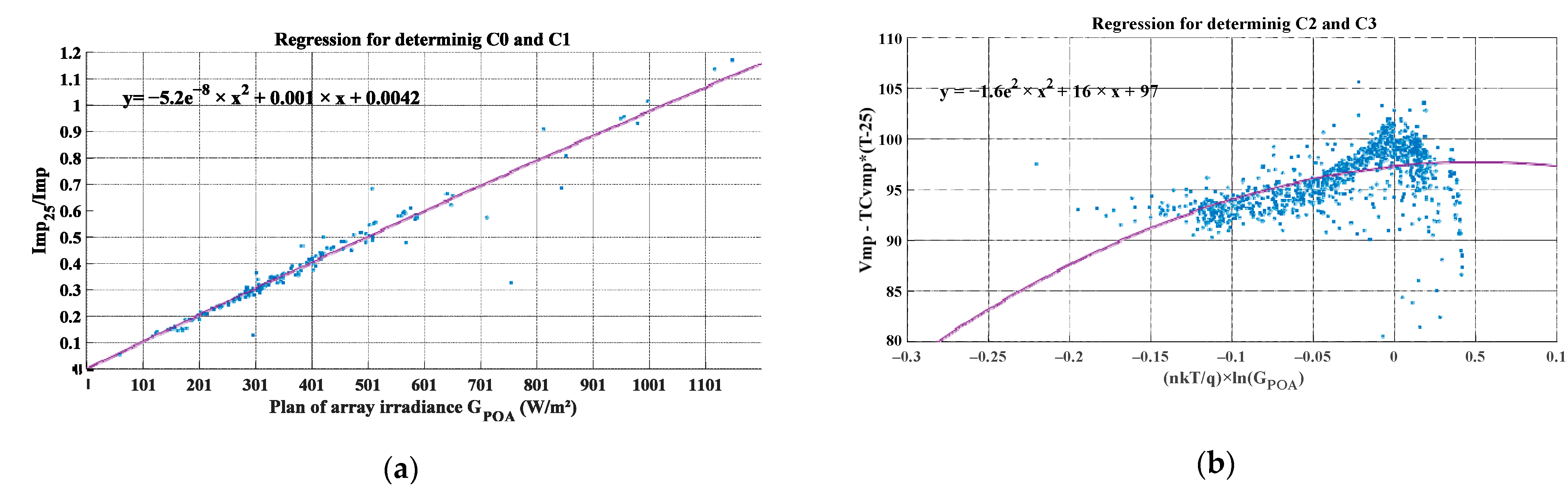
In this work, we applied monofacial electrical models to simulate the bifacial PV module energy production: (i) The model of Eduardo et al. [17], which uses the electrical characteristics indicated in the manufacturer datasheet at Standard Test Conditions (STC). (ii) The model of King et al. [18], known as the Sandia Array Performance Model, in which the model’s coefficients are determined from the assessment of the measured data. In both models, we considered that the short-circuit current and the current at maximum power point vary according to the backside power gain of the bifacial modules. The performances of the models were validated using measured data from monofacial and bifacial PV arrays installed in Barcelona, Spain.

The experimental setup was built up using the same commercial bifacial modules arranged in three PV arrays with the same configuration, such as the orientation, tilt, ground clearance, etc. However, the PV arrays were installed with different rear-side conditions; the backside of the first PV array was coated with a thin white plastic layer to provide data for monofacial operation. This was also considered as the reference PV array to allow an equivalent and direct evaluation of the advantage of the bifacial modules. The bifacial PV modules of the second and the third PV arrays were installed over normal and high albedos, respectively. The albedo of a surface corresponds to the ratio between the reflected light and the incident light. The albedo represents the amount of light reflected off of a surface. A dark body that absorbs light has low albedo, and a bright reflective body has high albedo [19].

Electrical, weather, and environmental conditions were measured by the installation of a number of sensors, such as pyranometers, thermocouples, current and voltage transducers, and others. We point out here that five irradiance sensors to measure the rear irradiance distribution of each albedo were installed. The developed monitoring program enabled the acquisition of all necessary data, the creation of daily XLS report files, and the visualization of all such data. The simulation results were compared with measurement data in order to evaluate the accuracy of models for bifacial applications.

2. Measurement Set-Up

The measurement set-up involved the design and installation of three bifacial PV arrays with a monitoring system capable of collecting weather, environmental, and electrical parameters. In order to provide comparative data under different rear-side conditions, we used the same bifacial PV module to form the PV arrays.

The arrays were installed on the flat roof of the Polytechnic University of Catalonia (UPC) in Terrassa (coordinates: 41°33′45.1″ N 2°1′15.5″ E), Spain. This setup belongs to the KETsupply pilot plant developed in the framework of the Sudoket Project, devoted to foster the application of Key Enabling Technologies (KET’s) in Intelligent Buildings [9,20]. The Azimuth of the building is 163°, which means it is rotated by 17° south-southeast. The bifacial PV module consists of 60 bifacial PERC cells (Passivated Emitter Rear Cell) encapsulated with EVA (Ethylene Vinyl Acetate) polymer and a front glass and rear glass. The nominal front side power is 320 Wp with a bifaciality of 70 ± 5%.

Table 1. The electrical parameters at Standard Test Conditions (STC) of the bifacial PV module with different irradiance conditions on the module’s backside; the rear-side power gain had a linear relationship to the parameters Isc and Imp, and Voc and Vmp were considered constant.

	Rear Side Power Gain
Parameters	Monofacial	5%	10%	15%	20%	25%
Cell efficiency, ηcell%	19.5
PV module efficiency, ηmodule%	19.2
Rated maximum power, Pmax Wp	320	336	352	368	384	400
Open circuit voltage, Voc V	40.79	40.80	40.80	40.80	40.90	40.90
Maximum Power Voltage, Vmp V	33.50	33.50	33.50	33.50	33.60	33.60
Short circuit current, Isc A	10.09	11.59	11.10	11.60	12.11	12.61
Maximum Power Current, Imp A	9.56	10.03	10.51	10.99	11.43	11.90
Temperature Coefficient of Isc, TCi%/°C	+0.060
Temperature Coefficient of Voc, TCv%/°C	−0.300
Temperature Coefficient of Maximum Power (Pmp), TCpmp%/°C	−0.370
Nominal Operating Cell Temperature, NOCT °C	45
Bifaciality (Pmprear/Rated Pmaxfront), Φ%	70

provides the bifacial module specifications under the STC with different levels of the backside power gain, these values were used to model the bifacial modules, see Section 3.

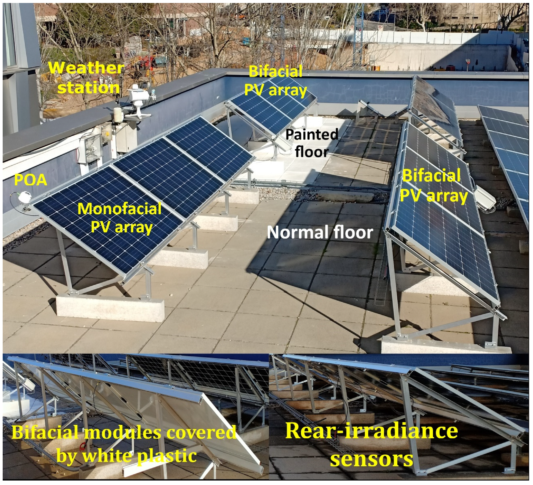
The bifacial PV modules were arranged in three PV arrays with 34° tilt, ground clearance height of 50 cm, and row-to-row distance of 3 m, see Figure 1. Each PV array was composed of three bifacial modules installed in a landscape position and connected in series; the rated power per array was 960 Wp. The landscape position reduced the non-homogeneity of the rear irradiance and provided a power gain. This landscape gain is defined as the power in landscape compared to portrait [21]. As shown in Figure 1, the bifacial modules were installed on the rooftop, where the natural floor provides a normal albedo for the bifacial modules, and the high reflectance floor provides a higher albedo due to paint with high solar reflectance index (SRI) of 105. The albedo is the reflected irradiance of the floor divided by the incident irradiance [22].

Before mounting the bifacial PV modules, three pyranometers were installed to measure the ground albedo: first, installed facing the sky, measuring the front incident irradiance, and the others facing the ground to measure the reflective irradiance of the normal and painted floors. We found that the albedo was 15% for the normal floor and only 32% for the painted floor, which was much lower than expected. As reported in [18], the albedo for concrete was 16%, and the addition of white paint increased the albedo to 62%. The same reported 23% for greenfield and 27% for white gravel. The albedo appeared to be highly affected by the surrounding structures, such as walls, PV arrays, buildings, and others.

In order to have the equivalent monofacial PV array (reference), the backside of the bifacial modules was covered with white plastic to obstruct the rear side of the bifacial cells. The same commercial bifacial module was used to reduce the differences due to cell and module technology. In [21], the researchers reported that the energy gain varied widely ranging from 13% to 35% and from 8.3% to 39%, respectively.

Figure 2 shows the testbed diagram developed to test and monitor the bifacial modules. The PV generation of each PV array was injected into the electrical grid by a single-phase PV inverter with a nominal power of 1.5 kW. As shown, the direct normal irradiance (DNI), global horizontal irradiance (GHI), plan of array irradiance (G_POA), and rear irradiance (Gr) for the normal and high albedos (Gr_NA and Gr_HA) were measured. Five sensors (EKO ML 01) were installed on the top, middle, and bottom to measure the reflective irradiance from the normal and painted floor. We also installed those for the normal albedo away from the reflection of the painted floor.

These measurements may allow us to study later the uniformity and distribution of the rear irradiance. The weather station also included sensors to measure the ambient temperature and humidity (Tamb and H) and an anemometer to measure the wind speed (W). The operating temperature of the PV modules (TC) was measured by fixing the thermocouples (type K) on the back of the central module for each PV array. The DC voltages and currents were measured by means of transducers installed at the output of each PV array; we indicate here that the inverter used had an MPPT efficiency of 99.9% and maximum efficiency of 97.1%. The information about the sensors and the measured parameters is summarized in

Table 2. Sensors and the measured parameters.

Parameter		Sensor	Accuracy/Precision	Input/Output
Solar irradiance	GHI	Pyranometer	0.5%	10.28 µV/W.m−2
	DNI	Pyrheliometer	0.5%	9.29 µV/W.m−2
	GPOA	Pyranometer	<1.5%	13.96 µV/W.m−2
	Gr	Si-pyranometer	<±2%	~50 µV/W.m−2
Temperature	Tc	Thermocouple K	±0.75%	±2.2 °C
	Tamb	HYGRASGARD® KFTF-I	±2%	4…20 mA/−35…+75 °C
Humidity	H		±1.8%	4…20 mA/0…100%
Wind speed	W	Anemometer	±0.5 m/s	0…100 Hz/0.8…40 m s−1
DC voltage	Vdc	Transducer	±1%	1000 V/5 V
DC current	Idc	Transducer	1%	±4 V/20 A

. The sensors were selected respecting the standard to monitor the performance of the PV system [23].

In order to ensure robust, reliable, and continuous measurement of the indoor and outdoor parameters, we designed the data acquisition system with two DAQs connected to the lab PC with Ethernet cables in a line topology. Then, using LabVIEW, we achieved a monitoring program that managed the DAQs to synchronize all the measured data from the sensors installed outside and inside the building. This system was also programmed to perform the calibration of the signals to the corresponding units, the real-time display of the measured and derived parameters, and the creation of the daily excel report files.

For the latter, a sub-program that saved all the measured parameters to an excel file at 30 s intervals was developed. At midnight, the sub-program reset all the energy meters, save and sent the daily excel file to a dedicated Dropbox, and created a new excel file for the next day. We directly saved the data to the Dropbox, which shared the files with the project team’s PCs; this prevented any data loss and full remote access to the database.

3. PV Module Models

In the current section, two monofacial performance models were used to simulate the power output of the bifacial arrays installed over different albedos as described above. We used an analytical model developed by Eduardo et al. [17] and an empirical model developed by King et al. [18] also known as the Sandia Array Performance Model. We selected these models due to their ability to model the full range of operating conditions (irradiance and temperature) and because they do not require additional parameters not specified in manufacturer data sheets. The PV module performance modeling is complicated by the influences of a variety of interactive factors related to the environment and solar cell physics. To monitor the performance of the PV arrays, a performance model must be able to separate and quantify the influence of all significant factors [18,24].

3.1. Analytical Model

The Equations (1)–(3) describe the PV module model defined by Eduardo et al. The analytical model takes into consideration the relationship of the current as a function of the voltage, the effective solar irradiance, the PV module operating temperature, the short-circuit current, the open-circuit voltage, and the performance coefficient of the PV module (b). The latter has a theoretical range between 0.01 and 0.18, where the smaller the b is, greater is the produced power [24]; Equation (4) describes how to calculate this coefficient. The variable ε is the maximum allowed error to stop the iteration; the performance coefficient is equal to 0.06074 for the installed bifacial PV module.

$$I\left(V\right)=\frac{Is{c}_x}{1-e^{(-\frac{1}{b})}}{ \times [1-e}^{\left(\frac{V}{b\times {Voc}_x}- \frac{1}{b}\right)}]$$

(1)

$$\begin{array}{c}{\mathit{Voc}}_x=s \times \frac{G_{POA}}{G_n}\times \mathit{TCv} \times \left(T_c-T_n\right){+ s \times \mathit{Voc}}_{\mathit{max}}- s \times \left({\mathit{Voc}}_{\mathit{max} }-{\mathit{Voc}}_{\mathit{min}}\right) \times \\ e^{\left(\frac{G_{POA}}{G_n} \times \mathit{ln}\left(\frac{{\mathit{Voc}}_{\mathit{max}} - \mathit{Voc}}{{\mathit{Voc}}_{\mathit{max}} - {\mathit{Voc}}_{\mathit{min}}}\right)\right)}\end{array}$$

(2)

$${\mathit{Isc}}_x=p \times \frac{G_{POA}}{G_n}\times \left[\mathit{Isc}+\mathit{TCi}\times \left(T_c-{ T}_n\right)\right],$$

(3)

while: $\left|b_{n+1}-b_n\right| > \mathsf{\epsilon }$

$$b_{n+1}=\frac{V_{\mathit{mp}}-{ V}_{\mathit{oc}}}{V_{\mathit{oc}}{ \times l}_n \left[1 -\frac{I_{\mathit{mp}}}{I_{\mathit{sc}}} \times \left(1 - \mathit{exp}\left(\frac{-1}{b_n}\right)\right) \right]}$$

(4)

where Isc_x and Voc_x are the short-circuit current and the open-circuit voltage considering the solar irradiance level (G_POA) and PV module operating temperature (Tc). Voc_max and Voc_min are the open-circuit voltages at 1200 W/m² and 200 W/m², respectively. In theory, Voc_max is close to 1.03 Voc, and Voc_min is close to 0.85 Voc [24]. Using the measured data in the MATLAB parameter estimation tool, the Voc_max was identified as equal to 1.02 Voc, and Voc_min was identified equal to 0.91 Voc. TCi is the temperature coefficient of Isc; TCv is the temperature coefficient of Voc. The nominal temperature (Tn) is equal to 25 °C; the nominal solar irradiance (Gn) is equal to 1000 W/m². Considering that PV modules have the same electrical characteristics, s and p are the numbers of PV modules connected in series and parallel, respectively.

The current and voltage at maximum power point (Imp_x and Vmp_x) were calculated directly using Equations (5) and (6), in which the dynamic limits of the IV curves (Isc_x and Voc_x) are calculated according to the solar irradiance and temperature of the module. This method, called the Linear Reoriented Coordinates Method [25], allows the estimation of the maximum output power without any defect, independently of the inverter algorithm.

$$Im{p}_x{ =\mathit{Isc}}_x\times \frac{1 -b+b \times \mathit{exp}\left(\frac{- 1}{b}\right)}{1 - \mathit{exp}\left(\frac{-1}{b}\right)}$$

(5)

$$Vm{p}_x{ =\mathit{Voc}}_x{+ b\times \mathit{Voc}}_x \times \mathit{ln}\left(b-b\times \mathit{exp}\left(-\frac{1}{b}\right)\right).$$

(6)

3.2. Empirical Model

The empirically based model defined by King et al. allows a direct prediction of the PV power output and takes into consideration the G_POA, Tc, and model coefficients as described by the following equations:

$$Im{p}_x=Imp\left(C0\times G_{POA}+C1\times G_{POA}^2\right)\left(1+TC{i}_{mp}\left(T_c-T_n\right)\right)$$

(7)

$$Vm{p}_x=Vmp+C2\times N_s\times \delta \left(T_c\right)\times \mathit{ln}\left(G_{POA}\right)+C3\times N_s\times {\left(\delta \left(T_c\right)\times \mathit{ln}\left(G_{POA}\right)\right)}^2+TC{v}_{mp}\left(T_n-T_0\right)$$

(8)

$$\delta \left(T_c\right)=n\times k\times \left(T_c+273.15\right)/q$$

(9)

where Imp_x and Vmp_x are the current and voltage at the maximum power point according to G_POA and Tc. Imp and Vmp are the current and voltage at the MPP under STC, respectively. Ns is the number of solar cells in series; δ(Tc) is the thermal voltage; n is the empirical diode factor; k is the Boltzmann’s constant; and q is the elementary charge. C0 and C1 coefficients relate Imp_x to the G_POA. The C2 and C3 coefficients relate Vmp_x to the G_POA.

The coefficients C0, C1, C2, and C3 were extracted using data measured in March and April in two different ways. First, C0 and C1 were obtained by a regression of Equation (7), the regression results are shown in Figure 3. C0 and C1 were found to be 0.001 and −5.2 × 10⁻⁹, respectively. C2 and C3 were obtained by a regression of Equation (8), and the regression results are shown in Figure 3. As C2 × Ns = 16, C3 × Ns = −1.6 10² and Ns = 160, C2 and C3 were calculated to be 0.01 and −0.89, respectively.

Second, we identified them directly by the well-known Levenberg–Marquardt and Trust Region estimation algorithms implemented in the MATLAB parameter estimation toolbox. This black-box method provides similar results (C0 = 0.001, C1 = 3.2 × 10⁻⁸, C2 = 0.012 and C3 = −0.73) to the regression of Equations (7) and (8). Nevertheless, more efforts were paid for the first method to process data; thus, we recommend the second method.

3.3. PV Module Bifaciality

In this sub-section, the fact that the bifacial PV module captures light from both the front and the rear sides (bifaciality) was integrated into the monofacial models presented above using the data sheet information and the measured front and rear irradiances (G_POA and Gr).

As shown in Table 1, the backside power gain had a linear relationship to the parameters Isc and Imp; therefore, they were introduced as variables to the models. The additional power generated by bifacial modules over monofacial modules is the bifacial gain, which is a metric for evaluating the performance of the bifacial PV module [26]. The bifacial gain is an electrical parameter; however, for a simple calculation of the output of the module, it can also be considered as an optical parameter while considering the values of the front and rear radiance [3]. As expressed in (10), we introduced the bifacial gain of irradiance (BGg) parameter to model the bifaciality of the modules.

$$B{G}_g=100\times \frac{G_r}{G_{POA}} \left(1-{\eta }_{loss}\right)$$

(10)

where the loss of power (η_loss) is caused by the non-homogeneity of the rear irradiance due to the shading and mismatch effects. The evaluation of similar bifacial PV systems in [27] showed that there was a neglected effect (<0.5%) on performance. However, by definition, rear non-uniformity is not more impactful to performance than front non-uniformity; however, due to reduced irradiance values in the rear, the non-uniformity effect decreases because the front irradiance still dominates strongly [3]. We assume that η_loss is equal to zero. Equation (11) expresses the BGg parameter used to calculate Isc and Voc with respect to the rear irradiance Gr.

$$B{G}_g=100\times \frac{G_r}{G_{POA}}.$$

(11)

For the analytical model, the Isc variable described in (12) was included in (3); for the empirical model, the Imp described in (13) was included in (7). The parameters Voc and Vmp are considered constant, and their values were selected from the monofacial test.

$$Isc=0.101 B{G}_g+10.09$$

(12)

$$Imp=0.0932 B{G}_g+9.56 .$$

(13)

In order to highlight the difference between normal and high albedo, the measured data of two months (54 days from 1 March to 29 April 2020) were organized according to the level of G_POA. The correlation in Figure 4 shows the behavior of the mean values, over the monitored period, of the received rear-irradiance energy (E_Gr) and the BGg with respect to the G_POA levels. As shown, BGg decreased as G_POA increased, and therefore BGg increased under low irradiance, reflecting the effects of weather conditions on the solar irradiance components [28,29].

As can be seen in Figure 4b, under G_POA greater than 400 W/m², the BGg was in the range between 2% and 6% for normal and high albedo, respectively. This was due to the low reflectivity of the floor under the bifacial modules as mentioned earlier in Section 2, and the albedos measured were 15% and 32% for the normal and the painted floors. The unexpected BGg measured will be investigated in further work related to the performance evaluation of bifacial modules requiring data from at least one year of monitoring.

4. Results and Discussion

The power outputs of the monofacial and bifacial PV arrays were simulated using the analytical and empirical models in which we introduced the ratio of Gr to G_POA (BGg) to integrate the behavior of the bifacial modules. The simulation results were compared to the measured data, we performed daily and monthly comparisons to discuss the precision of the models over different skies. Furthermore, we discussed the daily errors over the monitored period—six-months—to discuss the performance of the proposed models for bifacial applications with different albedos.

4.1. Daily Comparison

The PV output of the PV modules depends on the local climatic conditions; therefore, two typical weather conditions namely sunny-day and overcast-day, were considered for hourly simulation. Figure 5 and Figure 6 show the irradiances and temperatures over two days characterized by clear (07/03/20) and overcast (16/03/20) skies. During the sunny day, we observed that white paint greatly increased the rear irradiance of the bifacial modules installed above high albedo (Gr_HA) compared to the bifacial modules installed above normal albedo (Gr_NA). At noon, the Gr_HA max (89 W/m²) was three times the Gr_NA max (27 W/m²), see Figure 5a. The instantaneous BGg was close to 9% for high albedo and less than 3% for normal albedo, see Figure 5b. With the exception of low BGg values, the white paint greatly increased the solar irradiance on the backside of the bifacial modules.

Clearly, the operating temperature of the bifacial modules above high albedo was slightly higher than that of the others, which were superimposed as shown in Figure 5c. The max PV module temperature for high albedo was approximately 48 versus 42 °C for both monofacial and bifacial with normal albedo. These values were close to the NOCT of the PV module (45 °C) but are expected to be higher when the ambient temperature rises; the ambient temperature values were below 20 °C.

Instantaneous BGg values were particularly higher during the overcast day compared to the sunny day, as shown in Figure 6b. BGg values were higher than 5% and 10% for normal and high albedo, respectively, and were much higher during very low irradiance periods. This is due to the fact that the diffuse fraction (the ratio of diffuse irradiance and global irradiance) is high under low irradiance, which means that the available rear irradiance is more dominant in the total received irradiance compared to the clear sky [29].

As a result, the high BGg values will incorrectly amplify the simulated power output and, thus, reduce the accuracy of the proposed models under low irradiance conditions. However, the amount of energy received under overcast conditions was very low compared to sunny conditions. The operating temperature curves of all the PV modules were superimposed and ranged from 10 to 16 °C, see Figure 6c.

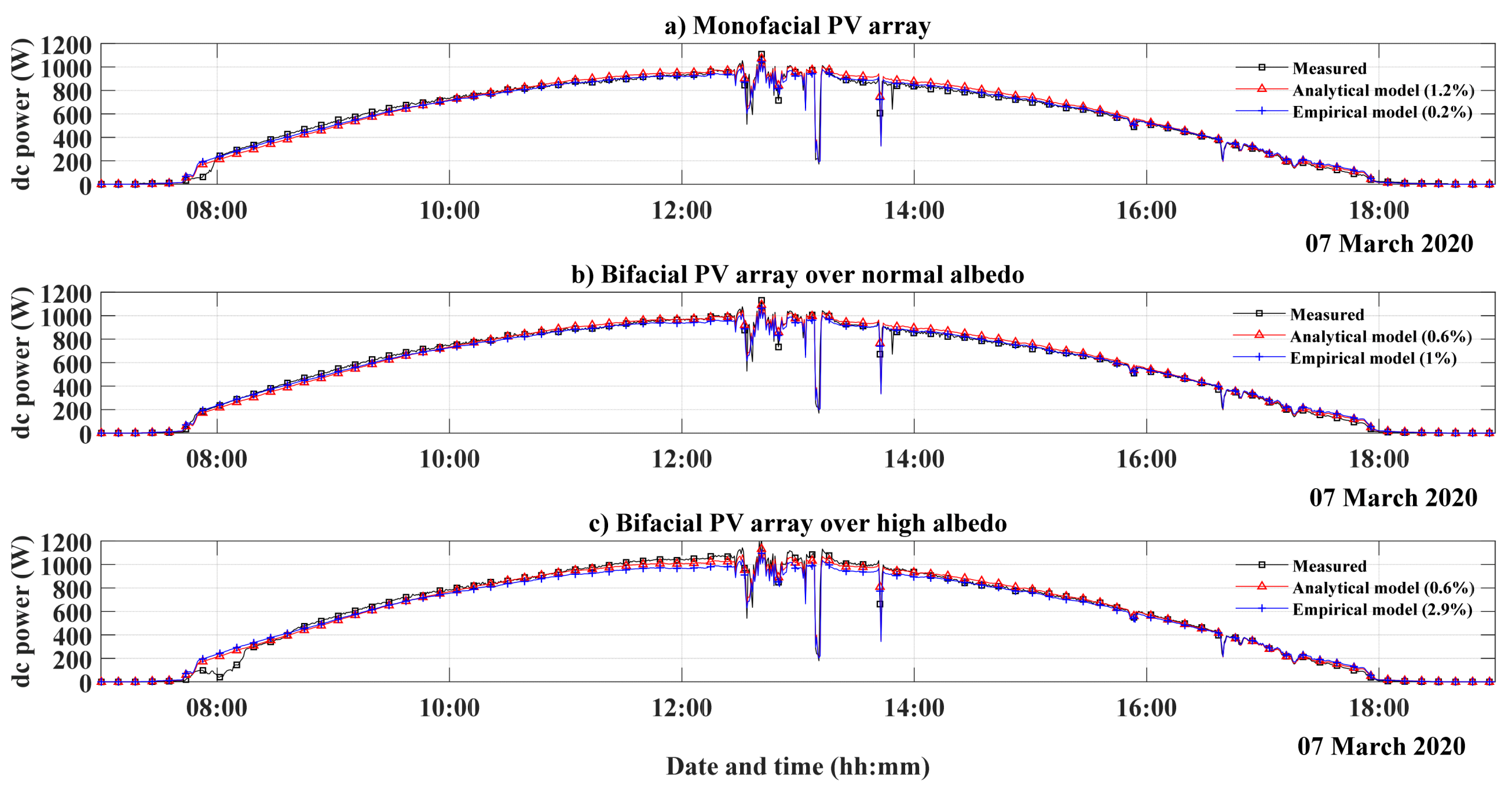
Figure 7 and Figure 8 show the simulation results of the analytical and empirical models applied to the monofacial modules and bifacial modules with different albedos. The models allow the dynamic behavior simulation of the monofacial and bifacial PV modules using the irradiances and PV module temperatures measurements. The comparison between the models shows that, for bifacial modules, the analytical model showed more accuracy than the empirical model. However, for monofacial modules, the empirical model showed better accuracy for sunny and overcast days, see Figure 7a and Figure 8a.

During the sunny day, the comparison results show that both models achieved good performance in terms of simulating the instantaneous power output of the PV arrays. The relative error of the models was calculated for the daily energy (measured and simulated); the errors on the sunny-day were much less than the overcast-day. Excluding the shading errors during the sunrise, shown in Figure 7a,c, we assume that the daily error of both models were found to be less than 1% for the sunny-day. The pyranometer was less affected than the PV arrays by the shading from the surrounding building.

During the overcast day, the relative errors were higher for both models, see Figure 8a–c. We can explain this for a number of reasons: First, we modeled the effect of the rear irradiance using the linear relationship between the Isc/Imp and the BGg (Equations (12) and (13)); therefore, the BGg caused a certain overestimation of the production of the bifacial modules under overcast conditions, as shown in Figure 8b,c. Second, the intense fluctuation of instantaneous solar irradiance (under overcast and cloudy conditions) also resulted in a relatively large measurement error (≥4%) between different instruments [30], and it could be interesting to assess the monitored data to correct the mismatches of the models.

Third, the DC voltage dropped by half during low irradiance periods, see Figure 9, which could be due to the maximum power point tracking (MPPT) algorithm of the PV inverters (SOLAX X1–1.5 kW). This was not considered in our model due to the lack of information on the PV inverter control strategy. Finally, the DC operating voltage (Vmp) of the PV arrays was close to 100 V during high irradiation and close to 50 V during low irradiance, which is much lower than the nominal DC operating voltage of the inverter (360 V). This may have an impact on the efficiency of the PV inverters, particularly during low irradiance periods.

4.2. Monthly Comparison

To evaluate the performance of the proposed models based on the heatmap visualization technique, we compared and evaluated the precision of the models (the difference between the measured and the simulated energy) using 166 days of measured data, from 1 March to 31 August 2020, which included spring and summer seasons.

Figure 10 shows the relative distribution of the rear irradiance energy (E_Gr) and the front irradiance energy (E_POA) of all monitored days on a heatmap. The map shows the distribution of days considering the normal and high albedos, the painted floor clearly increased the received irradiance (at the back of the bifacial modules) twofold; the distribution of the days on the map was more or less the same for both albedos. The heatmap can help to identify shading issues on both sides of the modules. As the building is south-southeast-facing, the backside of the bifacial modules could receive sunlight in the evening during the summer period. This is not the case due to the building located behind the bifacial PV arrays.

The maximum E_Gr values were measured during April and May, at more than 0.2 kWh/m²/day for the normal albedo and more than 0.4 kWh/m²/day for the high albedo. During June, July, and August, the sunlight was obstructed in the evening by the rear building, which affected the Gr received by the backside of the modules. The maximum E_Gr values were less than 0.1 kWh/m²/day for the normal albedo and less than 0.2 kWh/m²/day for the high albedo. The results showed that installation conditions, such as the azimuth angles of the sun and the surrounding obstacles, could have a strong impact on the energy received from the back of the modules.

Figure 11 shows the heatmap visualization of the daily relative errors for the monofacial modules; the simulation error results corresponding to the E_POA. As can be seen, most errors were less than 3% for the empiric model, and more than half were greater than 3% for the analytical model. The empiric model showed better precision for simulating the power output of the monofacial modules.

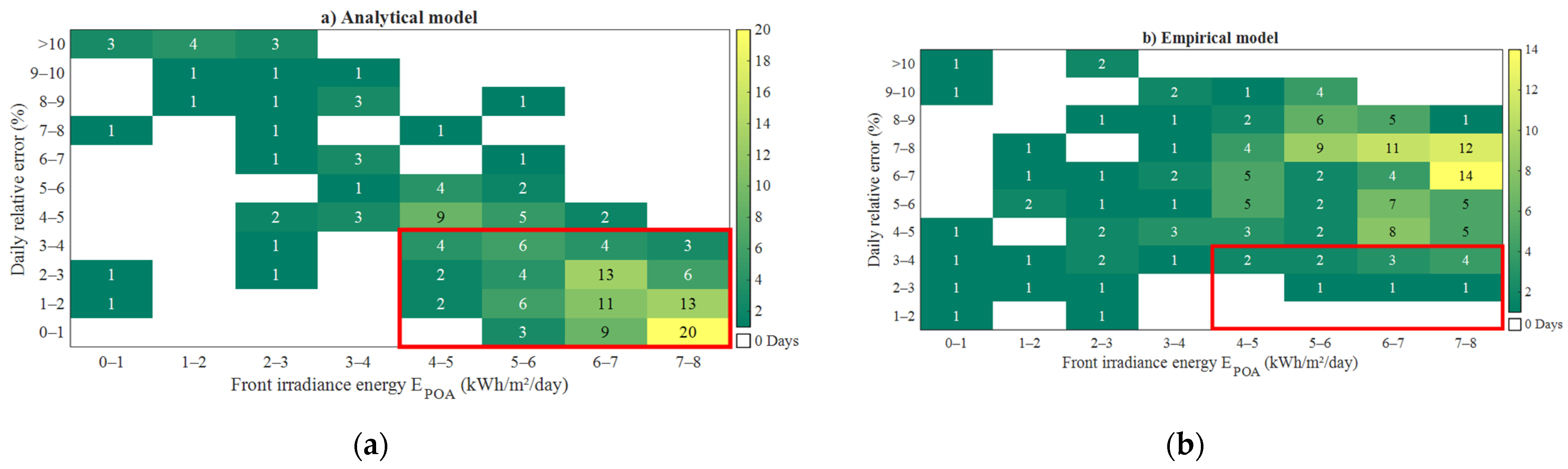
Figure 12 shows the heatmap visualization of the daily errors for the bifacial modules with normal albedo and the simulation error results corresponding to the E_POA. Unlike the monofacial modules, the maps show that the distribution of the daily errors was better for the analytical model. Within the highlighted area limited to E_POA more than 4 kWh/m²/day and relative errors less than 4%, the number of days for the analytical model and the empirical model were 125 and 114, respectively. In addition, there were 72 days with less than 2% error for the analytical model compared to 38 days for the empiric model.

Figure 13 shows the heatmap visualization of the daily errors for the bifacial modules with high albedo; the simulation error results corresponding to the E_POA. The distribution of the errors confirms the previous results. Within the same area (limited to >4 kWh/m²/day and <4%), the number of the days for the analytical model and the empirical model were 106 and 14, respectively. Under high albedo, the comparison between the maps shows the clear advantage to simulate the bifacial power output using the analytical model.

The bifacial energy gain was calculated by the ratio of the energy generated by the monofacial and bifacial PV arrays. As shown in

Table 3. Difference between the produced and the simulated energy over 166 days.

	Total DC Energy	Bifacial Energy Gain	Average Daily Error
			Analytical Model	Empirical Model
Monofacial PV array	792.95 kWh	/	2.44%	0.43%
Bifacial PV array with normal albedo	826.15 kWh	4.18%	0.51%	1.55%
Bifacial PV array with high albedo	868.77 kWh	9.56%	2.82%	5.28%

, the bifacial energy gain values for normal and high albedo were 4.18% and 9.56%, respectively. The results are approximately close to the values of the instantaneous BGg (bifacial gain of irradiance) under clear sky (9% for high albedo and less than 3% for normal albedo, see Figure 5). The average daily errors of the proposed models, given in Table 3, validate that the analytical model was more precise to simulate the bifacial PV production, with the daily average errors at 0.51% and 2.82% for normal and high albedos, respectively. However, the empirical model provided better accuracy to simulate the monofacial PV production, whose average daily error was 0.43%.

5. Conclusions

The simulation tools for bifacial PV generation are still under development, and their reliability needs to be demonstrated by comparison with the measured data. In this paper, we adapted two monofacial electrical PV models to simulate the power output of bifacial PV modules with different rear conditions. An experimental setup was built to demonstrate the feasibility of this approach by installing identical bifacial PV arrays with different albedos plus one monofacial PV array as a reference. Analytical and empiric models were used to simulate the instantaneous bifacial output of the modules by integrating the bifaciality of the modules (light capture from both front- and rear- sides) using the measured rear irradiance. The comparison with the monitored data showed that monofacial models could be a good way to monitor bifacial production.

The results showed very good agreement between the measured and the simulated results of the monofacial and bifacial modules under clear sky conditions. We found that the analytical model was more accurate and easier to implement compared to the empirical model. The latter was more accurate for monofacial simulation. As the models provide information on healthy operation using the measured solar irradiances and operating temperatures, we found that more than 2% of the differences under clear skies were due to the shading of the surrounding buildings.

These models integrated into the monitoring system could be an effective tool for assessing shading and soiling losses in real time. However, the accuracy of both models decreased under low solar irradiance conditions; thus, further work is planned to include the measurement of diffuse solar irradiance in the models. The assessment of the models over six months using the heatmap visualization technique confirmed the same results obtained from the instantaneous comparisons and provides us with a very powerful tool to show the effect of the albedo, the azimuth angles of the sun, and the surrounding obstacles.

The average daily errors for the analytical model were found to be less than 1% and 3% for normal and high albedos, respectively. This was achieved by accurate measurement of the solar irradiance and temperature, although further work could include other techniques/algorithms to avoid the expensive sensors and investigate the predictability of the bifacial production using monofacial models.