
Time-Dependent Climate Impact of Utilizing Residual Biomass for Biofuels—The Combined Influence of Modelling Choices and Climate Impact Metrics


Abstract
:1. Introduction
Aim and Scope
2. Materials and Methods
2.1. Biofuel and Reference Scenarios
2.1.1. Logging Residues
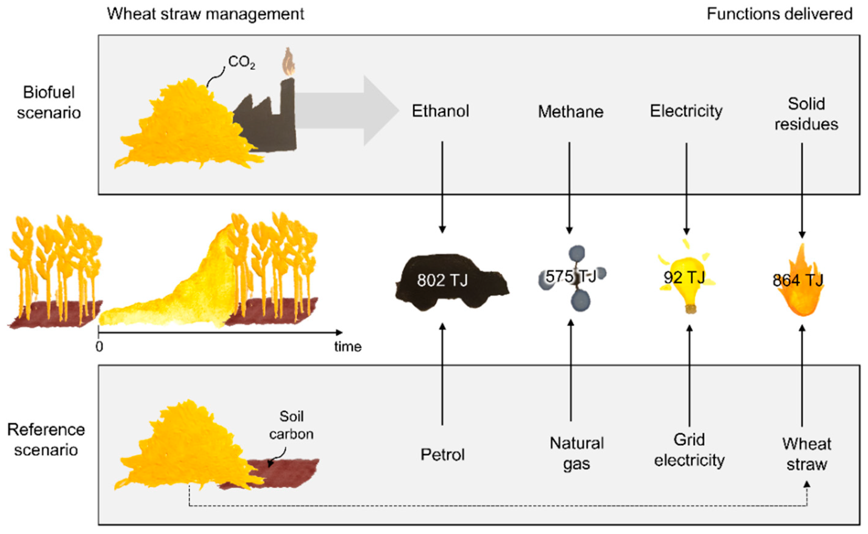
2.1.2. Straw
2.2. Temporal Considerations
2.2.1. Time-Dependent Carbon Flux in Biomass Life Cycles
2.2.2. Logging Residues
- Forest regrowth and carbon sequestration
- Decay of logging residues
- Soil organic carbon
2.2.3. Straw
- Soil organic carbon
2.3. Climate-Impact Assessment
2.3.1. Time-Aggregated Approaches
- Characterization factors for biogenic CO2
2.3.2. Time-Dependent Approaches
3. Results and Discussion
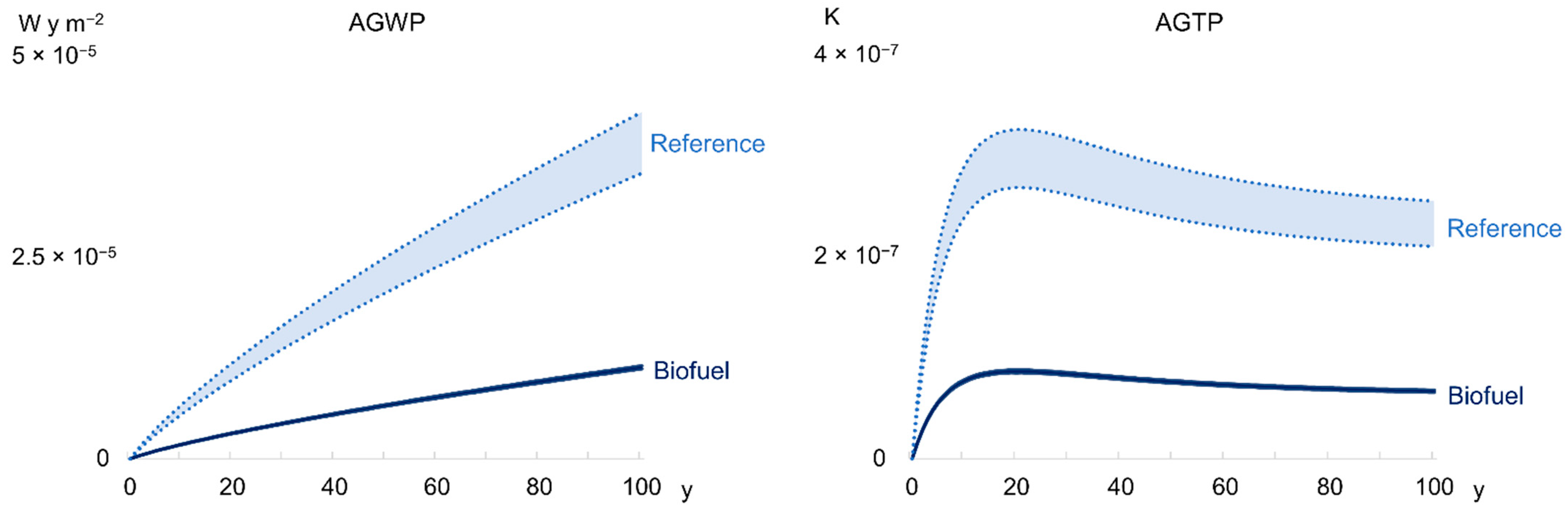
3.1. Logging Residues
3.1.1. Biogenic CO2 and Time-Dependent GHG Flux
3.1.2. Instantaneous and Cumulative Impact over Time
3.1.3. Parity Times
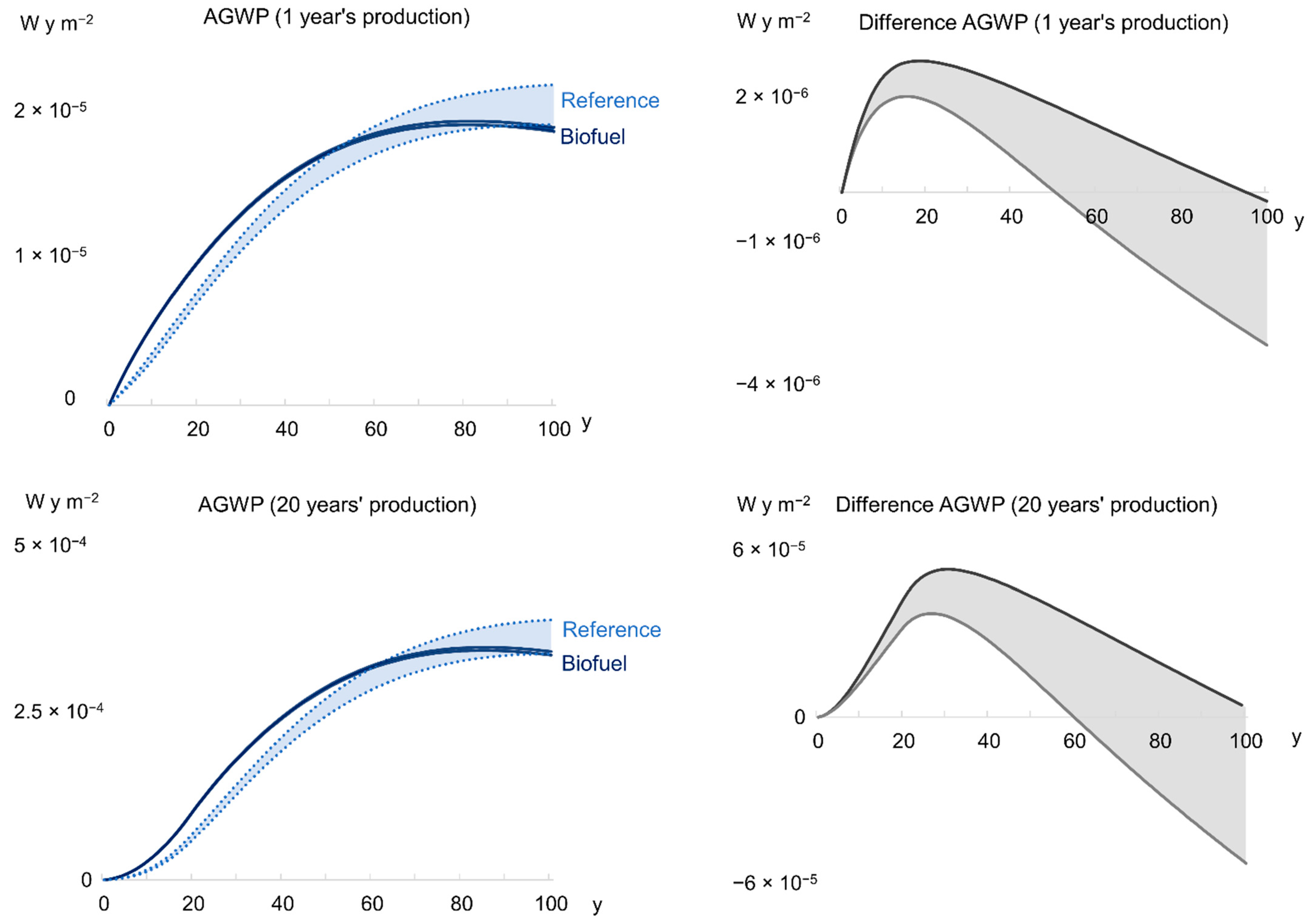
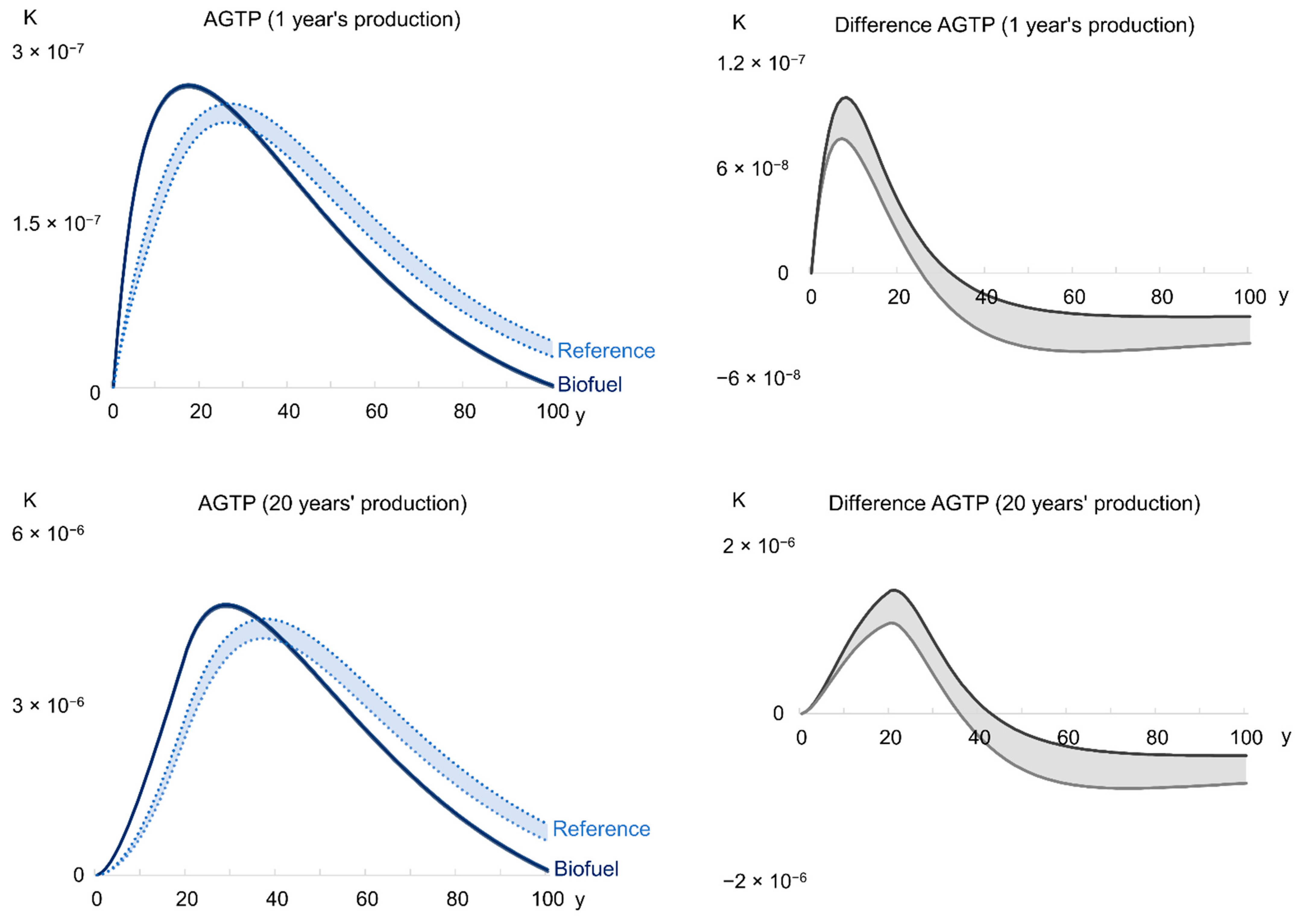
3.2. Straw
3.3. Limitations and Uncertainty
4. Conclusions
Supplementary Materials
Funding
Institutional Review Board Statement
Informed Consent Statement
Data Availability Statement
Conflicts of Interest
References
- McManus, M.C.; Taylor, C.M. The changing nature of life cycle assessment. Biomass Bioenergy 2015, 82, 13–26. [Google Scholar] [CrossRef] [PubMed] [Green Version]
- Lazarevic, D.; Martin, M. Life cycle assessment calculative practices in the Swedish biofuel sector: Governing biofuel sustainability by standards and numbers. Bus. Strategy Environ. 2018, 27, 1558–1568. [Google Scholar] [CrossRef]
- EC. Directive (EU) 2018/2001 of the European Parliament and of the Council of 11 December 2018 on the Promotion of the Use of Energy from Renewable Sources; European Commission: Brussels, Belgium, 2018. [Google Scholar]
- Finnveden, G.; Hauschild, M.Z.; Ekvall, T.; Guinée, J.; Heijungs, R.; Hellweg, S.; Koehler, A.; Pennington, D.; Suh, S. Recent developments in Life Cycle Assessment. J. Environ. Manag. 2009, 91, 1–21. [Google Scholar] [CrossRef] [PubMed]
- McManus, M.C.; Taylor, C.M.; Mohr, A.; Whittaker, C.; Scown, C.D.; Borrion, A.L.; Glithero, N.J.; Yin, Y. Challenge clusters facing LCA in environmental decision-making-what we can learn from biofuels. Int. J. Life Cycle Assess. 2015, 20, 1399–1414. [Google Scholar] [CrossRef] [Green Version]
- Lamers, P.; Junginger, M. The ‘debt’ is in the detail: A synthesis of recent temporal forest carbon analyses on woody biomass for energy. Biofuels Bioprod. Bioref. 2013, 7, 373–385. [Google Scholar] [CrossRef]
- Kendall, A.; Chang, B.; Sharpe, B. Accounting for Time-Dependent Effects in Biofuel Life Cycle Greenhouse Gas Emissions Calculations. Environ. Sci. Technol. 2009, 43, 7142–7147. [Google Scholar] [CrossRef]
- O’Hare, M.; Plevin, R.J.; Martin, J.I.; Jones, A.D.; Kendall, A.; Hopson, E. Proper accounting for time increases crop-based biofuels’ greenhouse gas deficit versus petroleum. Environ. Res. Lett. 2009, 4, 024001. [Google Scholar] [CrossRef]
- Cherubini, F.; Fuglestvedt, J.; Gasser, T.; Reisinger, A.; Cavalett, O.; Huijbregts, M.A.J.; Johansson, D.J.A.; Jørgensen, S.V.; Raugei, M.; Schivley, G.; et al. Bridging the gap between impact assessment methods and climate science. Environ. Sci. Policy 2016, 64, 129–140. [Google Scholar] [CrossRef] [Green Version]
- Azar, C.; Johansson, D.J.A. On the relationship between metrics to compare greenhouse gases—The case of IGTP, GWP and SGTP. Earth Syst. Dynam. 2012, 3, 139–147. [Google Scholar] [CrossRef] [Green Version]
- Farquharson, D.; Jaramillo, P.; Schivley, G.; Klima, K.; Carlson, D.; Samaras, C. Beyond Global Warming Potential: A Comparative Application of Climate Impact Metrics for the Life Cycle Assessment of Coal and Natural Gas Based Electricity. J. Ind. Ecol. 2017, 21, 857–873. [Google Scholar] [CrossRef]
- Lueddeckens, S.; Saling, P.; Guenther, E. Temporal issues in life cycle assessment—A systematic review. Int. J. Life Cycle Assess. 2020, 25, 1385–1401. [Google Scholar] [CrossRef]
- Beloin-Saint-Pierre, D.; Albers, A.; Hélias, A.; Tiruta-Barna, L.; Fantke, P.; Levasseur, A.; Benetto, E.; Benoist, A.; Collet, P. Addressing temporal considerations in life cycle assessment. Sci. Total Environ. 2020, 743, 140700. [Google Scholar] [CrossRef]
- Zanchi, G.; Pena, N.; Bird, N. Is woody bioenergy carbon neutral? A comparative assessment of emissions from consumption of woody bioenergy and fossil fuel. GCB Bioenergy 2012, 4, 761–772. [Google Scholar] [CrossRef] [Green Version]
- Norton, M.; Baldi, A.; Buda, V.; Carli, B.; Cudlin, P.; Jones, M.B.; Korhola, A.; Michalski, R.; Novo, F.; Oszlányi, J.; et al. Serious mismatches continue between science and policy in forest bioenergy. GCB Bioenergy 2019, 11, 1256–1263. [Google Scholar] [CrossRef] [Green Version]
- Helin, T.; Sokka, L.; Soimakallio, S.; Pingoud, K.; Pajula, T. Approaches for inclusion of forest carbon cycle in life cycle assessment—A review. GCB Bioenergy 2013, 5, 475–486. [Google Scholar] [CrossRef]
- Jolliet, O.; Antón, A.; Boulay, A.-M.; Cherubini, F.; Fantke, P.; Levasseur, A.; McKone, T.E.; Michelsen, O.; Milà i Canals, L.; Motoshita, M.; et al. Global guidance on environmental life cycle impact assessment indicators: Impacts of climate change, fine particulate matter formation, water consumption and land use. Int. J. Life Cycle Assess. 2018, 23, 2189–2207. [Google Scholar] [CrossRef] [Green Version]
- Levasseur, A.; Cavalett, O.; Fuglestvedt, J.S.; Gasser, T.; Johansson, D.J.A.; Jørgensen, S.V.; Raugei, M.; Reisinger, A.; Schivley, G.; Strømman, A.; et al. Enhancing life cycle impact assessment from climate science: Review of recent findings and recommendations for application to LCA. Ecol. Indic. 2016, 71, 163–174. [Google Scholar] [CrossRef] [Green Version]
- Brandão, M.; Levasseur, A.; Kirschbaum, M.U.F.; Weidema, B.P.; Cowie, A.L.; Jørgensen, S.V.; Hauschild, M.Z.; Pennington, D.W.; Chomkhamsri, K. Key issues and options in accounting for carbon sequestration and temporary storage in life cycle assessment and carbon footprinting. Int. J. Life Cycle Assess. 2013, 18, 230–240. [Google Scholar] [CrossRef]
- Laganière, J.; Paré, D.; Thiffault, E.; Bernier, P.Y. Range and uncertainties in estimating delays in greenhouse gas mitigation potential of forest bioenergy sourced from Canadian forests. GCB Bioenergy 2017, 9, 358–369. [Google Scholar] [CrossRef] [Green Version]
- Repo, A.; Tuomi, M.; Liski, J. Indirect carbon dioxide emissions from producing bioenergy from forest harvest residues. GCB Bioenergy 2011, 3, 107–115. [Google Scholar] [CrossRef] [Green Version]
- Bentsen, N.S. Carbon debt and payback time—Lost in the forest? Renew. Sustain. Energy Rev. 2017, 73, 1211–1217. [Google Scholar] [CrossRef]
- Hammar, T.; Stendahl, J.; Sundberg, C.; Holmström, H.; Hansson, P.-A. Climate impact and energy efficiency of woody bioenergy systems from a landscape perspective. Biomass Bioenergy 2019, 120, 189–199. [Google Scholar] [CrossRef]
- Hammar, T.; Levihn, F. Time-dependent climate impact of biomass use in a fourth generation district heating system, including BECCS. Biomass Bioenergy 2020, 138, 105606. [Google Scholar] [CrossRef]
- Karlsson, H.; Ahlgren, S.; Sandgren, M.; Passoth, V.; Wallberg, O.; Hansson, P.-A. Greenhouse gas performance of biochemical biodiesel production from straw: Soil organic carbon changes and time-dependent climate impact. Biotechnol. Biofuels 2017, 10, 217. [Google Scholar] [CrossRef] [PubMed]
- Sathre, R.; Gustavsson, L. Time-dependent climate benefits of using forest residues to substitute fossil fuels. Biomass Bioenergy 2011, 35, 2506–2516. [Google Scholar] [CrossRef]
- Giuntoli, J.; Caserini, S.; Marelli, L.; Baxter, D.; Agostini, A. Domestic heating from forest logging residues: Environmental risks and benefits. J. Clean Prod. 2015, 99, 206–216. [Google Scholar] [CrossRef]
- De Rosa, M.; Pizzol, M.; Schmidt, J. How methodological choices affect LCA climate impact results: The case of structural timber. Int. J. Life Cycle Assess. 2018, 23, 147–158. [Google Scholar] [CrossRef]
- Cooper, S.J.G.; Green, R.; Hattam, L.; Röder, M.; Welfle, A.; McManus, M. Exploring temporal aspects of climate-change effects due to bioenergy. Biomass Bioenergy 2020, 142, 105778. [Google Scholar] [CrossRef]
- Brandão, M.; Kirschbaum, M.U.F.; Cowie, A.L.; Hjuler, S.V. Quantifying the climate change effects of bioenergy systems: Comparison of 15 impact assessment methods. GCB Bioenergy 2019, 11, 727–743. [Google Scholar] [CrossRef]
- Fargione, J.; Hill, J.; Tilman, D.; Polasky, S.; Hawthorne, P. Land Clearing and the Biofuel Carbon Debt. Science 2008, 319, 1235–1238. [Google Scholar] [CrossRef] [Green Version]
- Searchinger, T.; Heimlich, R.; Houghton, R.A.; Dong, F.; Elobeid, A.; Fabiosa, J.; Tokgoz, S.; Hayes, D.; Yu, T.-h. Use of U.S. Croplands for Biofuels Increases Greenhouse Gases Through Emissions from Land-Use Change. Science 2008, 319, 1238–1240. [Google Scholar] [CrossRef] [PubMed]
- Röder, M.; Thiffault, E.; Martínez-Alonso, C.; Senez-Gagnon, F.; Paradis, L.; Thornley, P. Understanding the timing and variation of greenhouse gas emissions of forest bioenergy systems. Biomass Bioenergy 2019, 121, 99–114. [Google Scholar] [CrossRef]
- Campbell, B.M.; Beare, D.J.; Bennett, E.M.; Hall-Spencer, J.M.; Ingram, J.S.I.; Jaramillo, F.; Ortiz, R.; Ramankutty, N.; Sayer, J.A.; Shindell, D. Agriculture production as a major driver of the Earth system exceeding planetary boundaries. Ecol. Soc. 2017, 22. [Google Scholar] [CrossRef]
- Eriksson, L.; Klapwijk, M.J. Attitudes towards biodiversity conservation and carbon substitution in forestry: A study of stakeholders in Sweden. For. Int. J. For. Res. 2019, 92, 219–229. [Google Scholar] [CrossRef]
- Hanssen, S.V.; Huijbregts, M.A.J. Assessing the environmental benefits of utilising residual flows. Resour. Conserv. Recycl. 2019, 150, 104433. [Google Scholar] [CrossRef]
- Hammar, T.; Ortiz, C.A.; Stendahl, J.; Ahlgren, S.; Hansson, P.-A. Time-Dynamic Effects on the Global Temperature When Harvesting Logging Residues for Bioenergy. BioEnergy Res. 2015, 8, 1912–1924. [Google Scholar] [CrossRef] [Green Version]
- International Organization for Standardization (ISO). Environmental Management—Life Cycle Assessment—Requirements and Guidelines (ISO 14044:2006); ISO (International Organization for Standardization): Geneva, Switzerland, 2006. [Google Scholar]
- Tonini, D.; Hamelin, L.; Astrup, T.F. Environmental implications of the use of agro-industrial residues for biorefineries: Application of a deterministic model for indirect land-use changes. Glob. Chang. Biol. Bioenergy 2016, 8, 690–706. [Google Scholar] [CrossRef] [Green Version]
- Koponen, K.; Soimakallio, S.; Kline, K.L.; Cowie, A.; Brandão, M. Quantifying the climate effects of bioenergy—Choice of reference system. Renew. Sustain. Energy Rev. 2018, 81, 2271–2280. [Google Scholar] [CrossRef]
- Biograce. Harmonised Calculations of Biofuel Greenhouse Gas Emissions in Europe. Version 4d; Institute for Energy and Environmental Research (IFEU): Heidelburg, Germany, 2015. [Google Scholar]
- Edwards, R.; O’Connell, A.; Padella, M.; Giuntoli, J.; Koeble, R.; Bulgheroni, C.; Marelli, L.; Lonza, L. Definition of Input Data to Assess GHG Default Emissions from Biofuels in EU Legislation. Version 1d—2019; EUR 28349 EN; Publications Office of the European Union: Luxembourg, 2019. [Google Scholar]
- Barta, Z.; Kovacs, K.; Reczey, K.; Zacchi, G. Process design and economics of on-site cellulase production on various carbon sources in a softwood-based ethanol plant. Enzym. Res. 2010, 2010, 1–8. [Google Scholar] [CrossRef] [Green Version]
- Olofsson, J.; Barta, Z.; Börjesson, P.; Wallberg, O. Integrating enzyme fermentation in lignocellulosic ethanol production: Life-cycle assessment and techno-economic analysis. Biotechnol. Biofuels 2017, 10. [Google Scholar] [CrossRef] [Green Version]
- Arvidsson, R.; Tillman, A.-M.; Sandén, B.A.; Janssen, M.; Nordelöf, A.; Kushnir, D.; Molander, S. Environmental Assessment of Emerging Technologies: Recommendations for Prospective LCA. J. Ind. Ecol. 2018, 22, 1286–1294. [Google Scholar] [CrossRef] [Green Version]
- Karlsson, H. Climate Impact and Energy Balance of Emerging Biorefinery Systems. Ph.D. Thesis, Swedish University of Agricultural Sciences (SLU), Uppsala, Sweden, 2018. [Google Scholar]
- Gilpin, G.S.; Andrae, A.S.G. Comparative attributional life cycle assessment of European cellulase enzyme production for use in second-generation lignocellulosic bioethanol production. Int. J. Life Cycle Assess. 2017, 22, 1034–1053. [Google Scholar] [CrossRef]
- de la Fuente, T.; González-García, S.; Athanassiadis, D.; Nordfjell, T. Fuel consumption and GHG emissions of forest biomass supply chains in Northern Sweden: A comparison analysis between integrated and conventional supply chains. Scand. J. For. Res. 2017, 32, 568–581. [Google Scholar] [CrossRef]
- Lantz, M.; Prade, T.; Ahlgren, S.; Björnsson, L. Biogas and Ethanol from Wheat Grain or Straw: Is There a Trade-Off between Climate Impact, Avoidance of iLUC and Production Cost? Energies 2018, 11, 2633. [Google Scholar] [CrossRef] [Green Version]
- Levasseur, A.; Lesage, P.; Margni, M.; Samson, R. Biogenic Carbon and Temporary Storage Addressed with Dynamic Life Cycle Assessment. J. Ind. Ecol. 2013, 17, 117–128. [Google Scholar] [CrossRef]
- Albers, A.; Collet, P.; Benoist, A.; Hélias, A. Back to the future: Dynamic full carbon accounting applied to prospective bioenergy scenarios. Int. J. Life Cycle Assess. 2020, 25, 1242–1258. [Google Scholar] [CrossRef]
- Holtsmark, B. Quantifying the global warming potential of CO2 emissions from wood fuels. GCB Bioenergy 2015, 7, 195–206. [Google Scholar] [CrossRef]
- Yan, Y. Integrate carbon dynamic models in analyzing carbon sequestration impact of forest biomass harvest. Sci. Total Environ. 2018, 615, 581–587. [Google Scholar] [CrossRef]
- Gustavsson, L.; Haus, S.; Ortiz, C.A.; Sathre, R.; Truong, N.L. Climate effects of bioenergy from forest residues in comparison to fossil energy. Appl. Energy 2015, 138, 36–50. [Google Scholar] [CrossRef]
- Ågren, G.I.; Hyvönen, R.; Nilsson, T. Are Swedish forest soils sinks or sources for CO2—Model analyses based on forest inventory data. Biogeochemistry 2007, 82, 217–227. [Google Scholar] [CrossRef]
- Ortiz, C.A.; Liski, J.; Gärdenäs, A.I.; Lehtonen, A.; Lundblad, M.; Stendahl, J.; Ågren, G.I.; Karltun, E. Soil organic carbon stock changes in Swedish forest soils—A comparison of uncertainties and their sources through a national inventory and two simulation models. Ecol. Model. 2013, 251, 221–231. [Google Scholar] [CrossRef]
- Ranius, T.; Hämäläinen, A.; Egnell, G.; Olsson, B.; Eklöf, K.; Stendahl, J.; Rudolphi, J.; Sténs, A.; Felton, A. The effects of logging residue extraction for energy on ecosystem services and biodiversity: A synthesis. J. Environ. Manag. 2018, 209, 409–425. [Google Scholar] [CrossRef] [PubMed]
- Jurevics, A.; Peichl, M.; Egnell, G. Stand Volume Production in the Subsequent Stand during Three Decades Remains Unaffected by Slash and Stump Harvest in Nordic Forests. Forests 2018, 9, 770. [Google Scholar] [CrossRef] [Green Version]
- Björnsson, L.; Prade, T. Sustainable cereal straw management—Use as feedstock for emerging biobased industries or cropland soil incorporation? Waste Biomass Valorization 2021. [Google Scholar] [CrossRef]
- Buchspies, B.; Kaltschmitt, M.; Junginger, M. Straw utilization for biofuel production: A consequential assessment of greenhouse gas emissions from bioethanol and biomethane provision with a focus on the time dependency of emissions. GCB Bioenergy 2020, 12, 789–805. [Google Scholar] [CrossRef]
- Myhre, G.; Shindell, D.; Bréon, F.-M.; Collins, W.; Fuglestvedt, J.; Huang, J.; Koch, D.; Lamarque, J.-F.; Lee, D.; Mendoza, B.; et al. Anthropogenic and Natural Radiative Forcing. In Climate Change 2013: The Physical Science Basis. Contribution of Working Group I to the Fifth Assessment Report of the Intergovernmental Panel on Climate Change; Stocker, T.F., Qin, D., Plattner, G.-K., Tignor, M., Allen, S.K., Boschung, J., Nauels, A., Xia, Y., Bex, V., Midgley, P.M., Eds.; Cambridge University Press: Cambridge, UK; New York, NY, USA, 2013; pp. 659–740. [Google Scholar]
- Fuglestvedt, J.S.; Berntsen, T.K.; Godal, O.; Sausen, R.; Shine, K.P.; Skodvin, T. Metrics of Climate Change: Assessing Radiative Forcing and Emission Indices. Clim. Chang. 2003, 58, 267–331. [Google Scholar] [CrossRef]
- Shine, K.P.; Fuglestvedt, J.S.; Hailemariam, K.; Stuber, N. Alternatives to the Global Warming Potential for Comparing Climate Impacts of Emissions of Greenhouse Gases. Clim. Chang. 2005, 68, 281–302. [Google Scholar] [CrossRef] [Green Version]
- Cherubini, F.; Peters, G.P.; Berntsen, T.; Strømman, A.H.; Hertwich, E. CO2 emissions from biomass combustion for bioenergy: Atmospheric decay and contribution to global warming. GCB Bioenergy 2011, 3, 413–426. [Google Scholar] [CrossRef] [Green Version]
- Guest, G.; Cherubini, F.; Strømman, A.H. The role of forest residues in the accounting for the global warming potential of bioenergy. GCB Bioenergy 2013, 5, 459–466. [Google Scholar] [CrossRef] [Green Version]
- Liptow, C.; Janssen, M.; Tillman, A.-M. Accounting for effects of carbon flows in LCA of biomass-based products—Exploration and evaluation of a selection of existing methods. Int. J. Life Cycle Assess. 2018, 23, 2110–2125. [Google Scholar] [CrossRef] [Green Version]
- Pingoud, K.; Ekholm, T.; Savolainen, I. Global warming potential factors and warming payback time as climate indicators of forest biomass use. Mitig. Adapt. Strateg. Glob. Chang. 2012, 17, 369–386. [Google Scholar] [CrossRef]
- Ericsson, N.; Porsö, C.; Ahlgren, S.; Nordberg, Å.; Sundberg, C.; Hansson, P.-A. Time-dependent climate impact of a bioenergy system—Methodology development and application to Swedish conditions. GCB Bioenergy 2013, 5, 580–590. [Google Scholar] [CrossRef]
- Faraca, G.; Tonini, D.; Astrup, T.F. Dynamic accounting of greenhouse gas emissions from cascading utilisation of wood waste. Sci. Total Environ. 2019, 651, 2689–2700. [Google Scholar] [CrossRef] [PubMed]
- Levasseur, A.; Lesage, P.; Margni, M.; Deschênes, L.; Samson, R. Considering Time in LCA: Dynamic LCA and Its Application to Global Warming Impact Assessments. Environ. Sci. Technol. 2010, 44, 3169–3174. [Google Scholar] [CrossRef]
- Cooper, S. Temporal Climate Impacts; University of Bath: Bath, UK, 2020. [Google Scholar] [CrossRef]
- Allen, M. Short-Lived Promise? The Science and Policy of Cumulative and Short-Lived Climate Pollutants; Oxford Martin School, University of Oxford: Oxford, UK, 2015. [Google Scholar]
- de Jong, J.; Akselsson, C.; Egnell, G.; Löfgren, S.; Olsson, B.A. Miljöpåverkan av Skogsbränsleuttag—En Syntes av Forskningsläget Baserat på Bränsleprogrammet Hållbarhet 2011–2016; ER 2018:02; The Swedish Energy Agency: Eskilstuna, Sweden, 2018. [Google Scholar]


| Climate-Impact Metric | Life-Cycle Inventories | Biogenic CO2 | Climate Impact Metric | |||
|---|---|---|---|---|---|---|
| Time-Aggregated | Time-Dependent | Climate Neutral | Included | Cumulative | Instantaneous | |
| GWP | x | x | x | |||
| GTP | x | x | x | |||
| GWPbio a | x | x | x | |||
| AGWP | x | x | x | |||
| AGTP | x | x | x | |||
| CO2 | CH4 | N2O | Comment | Source | |
|---|---|---|---|---|---|
| GWP100 | 1 | 34 | 298 | With climate-carbon feedbacks a | [61] |
| GWP20 | 1 | 86 | 268 | ||
| GTP100 | 1 | 11 | 297 | ||
| GTP20 | 1 | 70 | 284 | ||
| GWPbio100 b | 0.43 | Rotation 100 years (LR c) | [64] | ||
| 0.53 | Rotation 100 years (LR c) and 75% harvest rate d | [65] | |||
| 0 | Rotation 1 year (WS e) | [64] | |||
| GWPbio20 b | 0.96 | Rotation 100 years (LR c) | [64] | ||
| 1.13 | Rotation 100 years (LR c) and 75% harvest rate c | [65] | |||
| 0.02 | Rotation 1 year (WS e) | [64] |
| Time Horizon | Climate-Impact Assessment | Unit | Biofuel Scenario | Reference Scenario | ||
|---|---|---|---|---|---|---|
| Low Case | High Case | Low Case | High Case | |||
| 100 years | GWP | Mt CO2-eq. | 16 | 19 | 91 | 100 |
| GTP | Mt CO2-eq. | 15 | 18 | 90 | 100 | |
| GWPbio | Mt CO2-eq. | 180 | 190 | 140 | 150 | |
| AGWP (1 year’s production) | W× year × m−2 | 1.9 × 10⁻⁵ | 1.9 × 10⁻⁵ | 1.9 × 10⁻⁵ | 2.2 × 10⁻⁵ | |
| AGWP (20 years’ production) | W × year × m−2 | 3.4 × 10⁻⁴ | 3.4 × 10⁻⁴ | 3.4 × 10⁻⁴ | 3.9 × 10⁻⁴ | |
| AGTP (1 year’s production) | K | 5.0 × 10⁻¹⁰ | 2.2 × 10⁻⁹ | 2.7 × 10⁻⁸ | 4.1 × 10⁻⁸ | |
| AGTP (20 years’ production) | K | 6.6 × 10⁻⁸ | 1.0 × 10⁻⁷ | 6.0 × 10⁻⁷ | 9.0 × 10⁻⁷ | |
| 20 years | GWP | Mt CO2-eq. | 16 | 19 | 94 | 110 |
| GTP | Mt CO2-eq. | 16 | 19 | 93 | 110 | |
| GWPbio | Mt CO2-eq. | 340 | 390 | 190 | 200 | |
| AGWP (1 year’s production) | W × year × m−2 | 9.8 × 10⁻⁶ | 9.9 × 10⁻⁶ | 7.1 × 10⁻⁶ | 7.8 × 10⁻⁶ | |
| AGWP (20 years’ production) | W × year × m−2 | 1.0 × 10⁻⁴ | 1.0 × 10⁻⁴ | 6.1 × 10⁻⁵ | 7.0 × 10⁻⁵ | |
| AGTP (1 year’s production) | K | 2.6 × 10⁻⁷ | 2.6 × 10⁻⁷ | 2.2 × 10⁻⁷ | 2.4 × 10⁻⁷ | |
| AGTP (20 years’ production) | K | 4.0 × 10⁻⁶ | 4.0 × 10⁻⁶ | 2.5 × 10⁻⁶ | 2.9 × 10⁻⁶ | |
| Time Horizon | Climate-Impact Assessment | Unit | Biofuel Scenario | Reference Scenario | ||
|---|---|---|---|---|---|---|
| Low Case | High Case | Low Case | High Case | |||
| 100 years | GWP | Mt CO2-eq. | 31 | 35 | 110 | 120 |
| GTP | Mt CO2-eq. | 30 | 34 | 100 | 120 | |
| GWPbio | Mt CO2-eq. | 31 | 35 | 110 | 120 | |
| AGWP | W × year × m−2 | 1.1 × 10⁻⁵ | 1.2 × 10⁻⁵ | 3.5 × 10⁻⁵ | 4.3 × 10⁻⁵ | |
| AGTP | K | 6.6 × 10⁻⁸ | 6.8 × 10⁻⁸ | 2.1 × 10⁻⁷ | 2.5 × 10⁻⁷ | |
| 20 years | GWP | Mt CO2-eq. | 34 | 38 | 110 | 130 |
| GTP | Mt CO2-eq. | 33 | 37 | 110 | 130 | |
| GWPbio | Mt CO2-eq. | 41 | 45 | 120 | 130 | |
| AGWP | W × year × m−2 | 3.1 × 10⁻⁶ | 3.2 × 10⁻⁶ | 9.8 × 10⁻⁶ | 1.2 × 10⁻⁵ | |
| AGTP | K | 8.5 × 10⁻⁸ | 8.8 × 10⁻⁸ | 2.7 × 10⁻⁷ | 3.3 × 10⁻⁷ | |
Publisher’s Note: MDPI stays neutral with regard to jurisdictional claims in published maps and institutional affiliations. |
© 2021 by the author. Licensee MDPI, Basel, Switzerland. This article is an open access article distributed under the terms and conditions of the Creative Commons Attribution (CC BY) license (https://creativecommons.org/licenses/by/4.0/).
Share and Cite
Olofsson, J. Time-Dependent Climate Impact of Utilizing Residual Biomass for Biofuels—The Combined Influence of Modelling Choices and Climate Impact Metrics. Energies 2021, 14, 4219. https://doi.org/10.3390/en14144219
Olofsson J. Time-Dependent Climate Impact of Utilizing Residual Biomass for Biofuels—The Combined Influence of Modelling Choices and Climate Impact Metrics. Energies. 2021; 14(14):4219. https://doi.org/10.3390/en14144219
Chicago/Turabian StyleOlofsson, Johanna. 2021. "Time-Dependent Climate Impact of Utilizing Residual Biomass for Biofuels—The Combined Influence of Modelling Choices and Climate Impact Metrics" Energies 14, no. 14: 4219. https://doi.org/10.3390/en14144219
APA StyleOlofsson, J. (2021). Time-Dependent Climate Impact of Utilizing Residual Biomass for Biofuels—The Combined Influence of Modelling Choices and Climate Impact Metrics. Energies, 14(14), 4219. https://doi.org/10.3390/en14144219