Abstract
In recent years, wind farm layout optimization (WFLO) has been extendedly developed to address the minimization of turbine wake effects in a wind farm. Considering that increasing the degrees of freedom in the decision space can lead to more efficient solutions in an optimization problem, in this work the WFLO problem that grants total freedom to the wind farm area shape is addressed for the first time. We apply multi-objective optimization with the power output (PO) and the electricity cable length (CL) as objective functions in Horns Rev I (Denmark) via 13 different genetic algorithms: a traditionally used algorithm, a newly developed algorithm, and 11 hybridizations resulted from the two. Turbine wakes and their interactions in the wind farm are computed through the in-house Gaussian wake model. Results show that several of the new algorithms outperform NSGA-II. Length-unconstrained layouts provide up to 5.9% PO improvements against the baseline. When limited to 20 km long, the obtained layouts provide up to 2.4% PO increase and 62% CL decrease. These improvements are respectively 10 and 3 times bigger than previous results obtained with the fixed area. When deriving a localized utility function, the cost of energy is reduced up to 2.7% against the baseline.
1. Introduction
Wind turbine wakes are responsible for considerable power losses in a wind farm (e.g., [1,2,3]), which can reduce power output up to 60% under certain wind directions and wind turbine alignments [4]. During the last two decades, wind farm layout optimization (WFLO) has been extendedly used to optimize the turbine positions in a wind farm, to minimize their wake effects and therefore improve its overall performance. Although numerous WFLO studies from multiple different perspectives have been carried out (see the review from [5] and references therein), a relevant WFLO question not sufficiently tackled so far arises on investigating which can be the most appropriate area shape for a wind farm in a future wind power project.
Within an optimization problem, increasing the degrees of freedom of the decision space can lead to the increase of the problem complexity (and therefore its computational cost), but also reach more efficient solutions (e.g., [6,7,8]). In the case of WFLO, the degrees of freedom can be raised through e.g., increasing the resolution of the search space, or removing constraints, such as that on the turbine hub height [9,10,11], the rotor diameter [12], or the wind farm boundaries. To this last respect, the possibility to optimize the wind farm shape has been traditionally neglected in the wind energy industry [13]. This is because usually wind farm projects are set up in two separate stages: first, the macro-siting stage takes place, where a certain delimited area is granted by the public administrations, according to public interest reasons such as environmental, safety and sea usage criteria [14]. Only after that stage is over, the micro-siting (layout design) stage takes place [15,16], and the layout of the turbines is set by the wind farm managers (with or without WFLO). This causes that the initial available area is usually not set according to wind farm performance criteria. For this reason, if the wind farm area shape and the turbine layout are optimized simultaneously within a single tool, it is reasonable to expect that a higher wind farm performance is attained, still respecting the conditions of the public administrations.
The literature involving the optimization of the wind farm area shape has been so far scarce. Some precursor works measure the used amount of surface (convex hull) by the wind farm, but keeping the boundaries fixed during the whole optimization [17,18]. Tong et al. [19] assessed a range of optimization-fixed rectangular wind farm aspect ratios and orientations (in separate runs), and highlight the sensitivity of the wind farm shape (in terms of the rectangle aspect ratio) to the overall performance compared to other design aspects. Stanley and Ning [12] carried out gradient-based WFLO on different design variables including the expansion of the area size, while keeping the same area shape unaltered. Finally, Wu et al. [13] proposed the single-objective optimization on the annual energy production, providing flexibility to the area of the wind farm, by allowing the optimization of the best performing parallelogram and orientation for the wind farm area shape. In this context, in this work we address the task to optimize the wind farm by completely removing any restriction on its area shape, at the time of involving multiple objective functions at a time.
In contrast to a single-objective optimization, multi-objective (MO) optimization problems [20,21] allow more than one objective (or cost) function to be optimized at a time. This results especially suitable for realistic problems, in which their complexity requires the optimization of multiple aspects. A certain problem is especially MO-suitable when its objective functions are not only independent, but also in conflict [22], so that the optimization of its objective functions is complementary (e.g., if one of them is single-optimized, the performance of the rest will tend to decrease). MO optimization has been used in many different fields, especially in problems involving some economic variable with a problem-specific feature, e.g., residential comfort [23], safety of infrastructures [24], energetic performance (e.g., [25]) or environmental objective functions (e.g., [26,27,28]), including those addressing wind power (e.g., [29,30,31]). Other fields in which MO optimization has provided successful insight include finance, (e.g., [32,33]), optimal control design (e.g., [34,35]) or industrial processes (e.g., [36,37]).
Regarding multi-objective WFLO (MO-WFLO), two variables that fall particularly in conflict when considering a variable (or unconstrained) wind farm area shape are the power output maximization (PO) and the electricity cable length (CL) reduction. In general, the fact of separating turbines in a wind farm will involve a PO increase due to the decrease in the impact of their wake effects, but also will imply a CL growth, which means an increased cost. This is in contrast with a fixed area WFLO, where results from single-objective PO optimization alone can involve systematic reductions in CL, usually producing solutions with turbines tending to locate on the wind farm perimeter (e.g., [38,39]). During the last decade, several MO-WFLO works have been produced, most of them comparing the wind farm energy production (or output power) against another objective function, such as the level of noise [40,41,42] an objective function of constraints [43], or the economic cost (e.g., [38,44,45,46,47]). Using economic objective functions during the optimization has the associated problem that they are subject to the continuous change in the local and global economy. To this regard, some studies have compared non-economic variables as PO against CL (as the aforementioned scheme) [17,18,48,49]. In turn, a few MO-WFLO works have compared energy or power with more than one aspect. For instance, in addition to CL, Li et al. [17] compares power to the used area in an independent exercise, whereas [18] consider energy production against CL, used area and an environmental impact as three different additional objective functions (as emphasized above, in these works the wind farm area limits are kept fixed throughout the whole evolution).
Regarding the optimization technique applied, some WFLO works have used deterministic methods (e.g., [11,50,51,52,53]). However, most contributions have done so by means of stochastic optimization. From these, most have relied on meta-heuristic techniques such as ant colony optimization [54], particle swarm [55,56,57] or the most largely used, evolutionary (or genetic) algorithms (e.g., [39,58,59,60,61,62,63,64,65]). Stochastic optimization has been shown well suited for WFLO, as they allow exploring large search spaces without the need to assess every single wind farm solution therein. This suitability has been especially proven in combination with objective functions that include the use of an analytical model to represent wind turbine wakes [66,67,68], as their computational simplicity allows assessing multiple (thousands) of wind farm potential solutions in a reasonable time.
In this work, we address the multi-objective CL vs. PO problem by performing a fully unconstrained (free) wind farm area shape optimization (i.e., without any a priori predefined family of shapes), by means of a newly developed, shape self-adaptive MO optimization procedure. In addition, we conceive that the developed routine must keep the total available area (in terms of km) constrained, to keep the same amount of sea surface usage, and to ensure that any potential improvement is due to the shape optimization instead of a mere area increase. Here we design a novel MO, WFLO-oriented algorithm inspired by our previous algorithm in [39], and compare it to the Non-dominated Sorting Genetic Algorithm version II (NSGA-II [69]), a MO algorithm widely used in the context of industrial processes [36,37,70], including those considering wind energy (e.g., [40,71]). Furthermore, a set of 11 additional algorithms, with different variations from the two are also developed and tested. All the algorithms are applied under a realistic framework, i.e., considering a high-resolution wind climatology and infinitesimal turbine positioning ability, factors that have been shown crucial when aiming to obtain reliable wind farm layouts and non-spurious performance [39,49,72]. In addition, our PO objective function uses the analytical wake model from the (hereafter the EPFL Gaussian model [68]), which has shown higher accuracy than other models traditionally employed. In the last part of the article, after the MO optimization, an economical utility function with the particularities of a local decision maker is derived and implemented on the solutions obtained during the MO optimizations.
2. Methodology
2.1. Analytical Modelling of the Wind Farm Flow
The high variability of the near-surface wind requires assessing multiple different wind directions and magnitudes for a given wind farm, to obtain a realistic insight of its wind power capability [4,73,74]. On the other hand, a WFLO problem usually requires assessing at least tenths of thousands of different wind farm layout configurations. This framework is far from being computationally feasible with the usage of computational fluid dynamics simulations (e.g., large eddy simulations, LES) to model the wake interactions in a wind farm. This caveat can be overcome through the implementation of simple and computationally inexpensive analytical wake models, where time-averaged flow conditions are calculated through simple analytic expressions and only over the specific points of interest inside a wind farm (essentially in front of the downstream turbines affected by a wake). Traditionally, very simple analytical top-hat profile wake models have been applied (especially [66] but also [67]) due to their simplicity, practicality and being computationally very cheap. In recent years, based on the idea of self-similarity in a wake, a Gaussian-profiled wake model has been developed [68,74] which satisfies the conservation of mass and momentum in the far wake flow. This, added to the fact that this model has shown higher accuracy than previously and traditionally used models [66,67], led us to consider it for this work. According to it, the velocity deficit , normalized with respect to the incoming velocity , can be defined as follows (see [68] for details on its derivation):
where x, y and z are the streamwise, spanwise and vertical coordinates, respectively, is the hub height, represents the growth rate of the wake, stands for the thrust coefficient of the turbine, D is the turbine rotor diameter and represents the initial wake expansion parameter.
The resulting incoming wind speed in a turbine j in a wind farm must consider the contribution of all wind speeds in all the turbines i located upstream from it, as well as their interactions, . Niayifar and Porté-Agel [74] showed that the linearization of the wake superposition, inspired by the pollution plume mass conservation shown in [75], produced best validation results against LES experiments [76] compared to other approaches, and thus became the scheme followed in this work:
where is the wake velocity of turbine i in the position of turbine j. Finally, a value of power output is assigned to each velocity obtained, according to the power curve corresponding to the considered turbine model. Studies based on LES [76] and scanning wind LiDARs [77] have shown that the growth rate k* of a wake produced by a turbine j can be associated with the turbulence intensity level I immediately upwind the turbine rotor. In this work we consider the linear relationship derived empirically between k* and I derived by [74]. Finally, the turbine added turbulence intensity, i.e., the increase of the turbulence intensity level produced by each turbine rotor in the wind farm, is defined by the expression proposed by [78].
2.2. Multi-Objective Wind Farm Layout Optimization (MO-WFLO)
Although some single-solution MO algorithms can be found in the literature (e.g., [79]), most MO algorithms provide a wide range of solutions, in which the obtained values of their objective functions gradually change. This means that the set of solutions transits from solutions entirely optimized only for one of the objective functions (but are least optimized for the rest of objective functions), until some intermediate solutions that have all objective functions optimized approximately at the same level. Decision variables of each solution x are represented in the decision space , whereas the values of the M objective functions for each solution x, F(x) = (,), are represented on the objective space . The intersection of the two optimal objective functions (i.e., here and ) at the objective space (see Figure 1) defines the ideal objective vector (IOV).
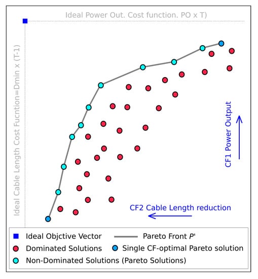
Figure 1.
Scheme of the MO-WFLO objective space considered in this work.
Most MO algorithms generate their range of solutions according to the so-called Pareto fronts [80] over the space (see e.g., [81]). Here, for each solution x (i.e., each possible wind farm layout), decision variables , , represent the vector positions of the T turbines in the wind farm, whereas the objective function values for that solution are F(x) =(,).
Pareto fronts are based on the concept of non-domination [20,21,82]. Non-domination is an objective method that compares each solution with the rest, extracting those solutions that are better performing. A certain solution x is said to be non-dominated with respect to any solution x’ ( i.e., x ⪯ x’) if there is no x’ that outperforms x on all objective functions at the same time. The Pareto front is thus defined by the front of size in the space formed by the objective function values whose associated solutions are non-dominated by any other solution x’:
Formally, if a set of solutions is non-dominated with respect to the whole number of existing solutions , the Pareto front is said to be optimal. As we will refer exclusively to non-dominated solutions within this case, hereafter it will be just referred to as the Pareto front . Here, non-domination refers to those solutions strictly better performing than all the rest of solutions in at least one of the objective functions CL or PO. The MO-WFLO framework applied in this work is illustrated in Figure 1. As any MO optimization, here the Pareto front is to be evaluated at every time step and updated with any new solution (here F(x) = (,)) that fulfills the Pareto front definition. After reaching some termination condition, the attained set of solutions provided by during the MO optimization is delivered to a decision maker (stakeholders, institutions, etc.) which evaluates them and eventually selects a final one according to its particular requirements.
2.3. Formulation of the MO-WFLO Problem
As argued in the introduction, an unconstrained (variable) area shape approach of the WFLO problem can stimulate the conflict between CL reduction and PO increase, thus making it especially appropriate for MO optimization. Following this idea, here we address a MO-WFLO with the PO maximization and CL minimization as objective functions. PO can be defined as the overall output power in all turbines throughout multiple wind speeds and directions defining its climatology, as follows:
being the power output of turbine t in a wind farm with a T turbines, according to the incoming wind speed b and angular sector s of a wind rose with S sectors and B speed bins per sector. The power curve (normally provided by the turbine manufacturer) provides the power generated by the turbine as a function of the incoming wind velocity [83]. Here is derived by applying the turbine power curve to the corresponding incoming wind velocity obtained with the wake model. In turn, the CL objective function is computed by means of the minimum spanning tree function [84].
WFLO problems can be subject to multiple constraints. However, two of them are present in most WFLO contributions, one being related to the minimum distance between turbine rotors, and the other one linked to the spatial limitation of the wind farm area, usually in both shape and size. Here, the spatial constraint related to the wind farm area becomes only linked to the maximum size of the wind farm , whereas its boundaries do not entail anymore a proper constrain, but are permanently updated during the optimization process. The wind farm area is determined by the convex hull of the turbine positions according to the algorithm from [85]. In this work we allowed a fully unconstrained area shape variation while continuously keeping the amount of original area (in km) constrained, to ensure that the potential benefit of the optimization was due exclusively to the area shape variation and not to an area size increase. To attain this, we developed a self-adaptive area updating routine at each generation, which was applied to all the algorithms considered. Specifically, the area update takes place after crossover and mutation, where three options are possible for an individual (for ) regarding its relative size with respect to the maximum area constraint, :
- <An area is defined through the expansion of until reaching size, while keeping its shape proportional to the original area. This area will be used as limit for any new position of those turbines which need to be relocated (if any) due to a violation of the constraint.
- >The is updated by shrinking its size until reaching , while keeping the shape proportional to the original area. This area will be the limit for those turbines which need to be relocated (if any) due to a violation of the constraint, and for those turbines which are left out of the new area.
- =No action is taken.
With all the above, the variable-shape (hereafter VariShape) MO-WFLO problem can be formulated as follows:
- : Maximize PO: .
- : Minimize CL: minimum spanning tree.
- Constraint for the minimum distance X between turbines:
- Constraint for the maximum area: .
As a reference for the optimization performance, the optimal attainable values for the objective functions alone can be defined. The minimum CL () is ruled by the distance constraint between two turbines, , whereas the maximum attainable PO () represents a situation where no wake effects are involved, hence defined by the power output of a wind turbine alone times the amount of turbines considered, so that .
2.4. MOEA Optimization Algorithms
Since their proliferation in the 1990s, population-based algorithms as evolutionary (or genetic) algorithms have been the most largely used algorithm types for MO optimization (e.g., [69,86,87], Coello et al. [81] and references therein). This is related to the fact that population-based algorithms such as MO evolutionary algorithms (MOEA) are capable of generating multiple solutions of a complex problem, which allows an evolving of the Pareto front in a balanced trade-off between the different objective functions involved [88].
MOEAs, and evolutionary algorithms in general, are characterized by evolving their population throughout a series of generations (iterations), until a termination condition is encountered, and the best performing individual (solution) (or set of individuals) at the last generation is retained. Each of these iterations typically involve a series of steps, namely fitness, selection and breeding (generally including crossover and mutation operators).
In this work, a set of 13 different MOEAs is considered, 12 of them being newly developed here. The set of MOEAs includes:
- The NSGA-II [69] algorithm.
- A newly designed MOEA inspired by the crossover-elitist genetic algorithm (CEGA) [39], (hereafter V-CEGA).
- A set of 11 additional algorithms, mainly resulting from the hybridization of NSGEA-II and V-CEGA, or to a lesser extent from small variations from V-CEGA or NSGA-II.
For all of them, a population size (N) based on evolution efficiency was set to 300 individuals (in the order of the amount in [39]). Additionally, a preset termination condition consisting of a running time limit of 144 wall clock hours (8640 min.) was applied to all algorithms, to ensure their equal performance opportunity. Following, the main particularities of the considered algorithms (selection, breeding and structure) are described.
2.4.1. NSGA-II Algorithm
The NSGA-II [69] algorithm, a MOEA widely used for energy optimization processes (e.g., [70,71]) including WFLO (e.g., [40]), is characterized by arranging its solutions in the objective space according to subsequent non-dominated fronts to grant elitism. During selection, in first place the Pareto front is computed, and the individuals belonging to that front are selected. Subsequently, those solutions are omitted and the new front computed, and its members selected. This operation is carried out n times until the sum of the individuals selected reaches or exceeds the number of elements required. On the last front, the exceeding elements (if any) are dismissed according to their crowding distance, and the individuals with smallest distance between them and the surrounding solutions are dismissed (see [69] for more details).
NSGA-II works (in real-coded algorithms) with a simulated binary crossover (SBX, [89]) and polynomial mutation (PMUT) as breeding operators [90]. In addition, it has an algorithm structure in which, in each generation, the selection is computed after the breeding, extending the population from N to during the breeding, and reducing it again to a size of N after the selection. For this work, probabilities p and distribution indices for crossover c and mutation m were set following [69], namely = 0.9, = 0.1 and = = 20.
2.4.2. Vertex-Selection Crossover-Elitist Genetic Algorithm (V-CEGA)
A new MO algorithm was designed for this work, to adapt the WFLO problem to MO optimization. The algorithm is inspired by the CEGA algorithm from [39] (V-CEGA algorithm, V for selection), with a newly introduced selection procedure adapted to MO optimization. Following, details on the selection and breeding (crossover and mutation operators) applied at each generation are provided:
- SelectionOnce the objective functions have been evaluated for all individuals and their values are deployed throughout the objective space, a few of them are selected to generate new offspring individuals. The number of selected individuals is defined by the population size N and the generation gap , so that . Following [39,91] a value of = 0.9 was set for V-CEGA, this meaning that at each generation 10% of the population is selected, whereas the dismissed 90% need to be renewed. Once N and are set, the V-CEGA selection follows a self-adaptive scheme with two possible procedures depending on the amount of non-dominated solutions at the Pareto front. If , then the whole Pareto front is selected, as well as the F() solutions nearest to any solution F(). If on the contrary (which is most usual), in first place the algorithm systematically selects three points in the objective space: the two Pareto front solutions that are optimal at each objective function individually (vertices ,), plus the Pareto solution showing the minimum distance to the Ideal Objective Vector (IOV, here equal to (,)), namely the frontal vertex . To ensure that the selection of is kept independent from the possible difference of magnitudes of the two objective functions, is defined after normalizing the objective space. This normalization (Figure 2) is performed with respect to the distances form and to IOV, respectively and , so that they are similar after the normalization. To achieve that, the x coordinates of the solutions in the objective space (PO values in this case) are multiplied by the ratio, so after that (the distance between the new vertex position and IOV) is equal to . In second place, further (dominated) solutions F() are randomly selected until the selection size () is reached. To harness all non-dominated solutions from past generations, if an individual F() is not selected in a past generation but still represents a non-dominated solution in the following generation (after fitness), it is reinstated into the Pareto Front, and therefore susceptible to be selected and become part of .
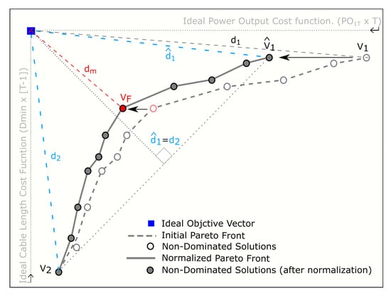 Figure 2. Scheme of the computation of .
 - BreedingDuring the breeding, which in this work involves both crossover and mutation, new individuals are created from the selected population until the population size N is restored. In V-CEGA, the breeding procedures have been preserved identically as in CEGA [39]. During the CEGA crossover, which is especially conceived for the WFLO problem, each of the new individuals (here 90% of the population) are created from two parents randomly chosen from the selected ones (here 10%). The way the information from the two parents is used to create the offspring is based on elitist criteria, which relies on the relative power output of each turbine with respect to the rest. The crossover is controlled by a single parameter , which indicates the fraction of PO with respect to the most performing turbine at the individual with the higher power output, and is used as a threshold. The turbines at which exceed that threshold are retained. Finally, the rest of turbines remaining to reach the number of turbines T in the wind farm are those turbines at which are placed closest to the dismissed ones in .Following the crossover, a certain amount of mutation is introduced to the individuals to enrich the population diversity. In this way, each offspring has a certain probability of being mutated. In turn, each turbine at a mutating individual has a probability of varying its position a distance (in m). With respect to its original position , a mutated turbine position is defined as:where (q = 1, 2, 3, 4) are random numbers belonging to the uniform distribution . The breeding operators and , and were set respectively to 0.9, and 0.99, 0.8 and 70 following the CEGA parameterization in [39]. After breeding, a new generation is fully set, and the new elements are ready to be submitted to fitness.
2.4.3. Hybrid Algorithms and Variations from V-CEGA and NSGA-II
V-CEGA has three main elements that are substantially different with respect to NSGA-II. In first place, in V-CEGA breeding is adapted to the WFLO problem, with a strategy that allows chromosome elitism inside the wind farm (only low performing turbines are ‘moved’ to positions provided from the other parent) and has proven highly effective [39] Secondly, selection is clearly different, as shown in the previous sections. Finally, the algorithm structure is different: in V-CEGA the structure is Fitness-Selection-Breeding, with a 10% selected population that recovers the initial population N during breeding. On the contrary, NSGA-II has a Breeding-Fitness-Selection structure, with population increasing momentarily to during breeding, to be reduced again to N during selection. To investigate the behavior of each of these three elements (breeding, selection and structure), a series of hybrid algorithms have been developed by combining these three components from V-CEGA and NSGA-II one by one. This provided an overall of 6 hybrid algorithms (see Table 1).

Table 1.
Summary of the key features of the set of designed algorithms.
In addition to these, other algorithms with smaller variations where derived. For comparison. versions of V-CEGA and NSGA-II were also set up with a single point crossover (SPX, [89]), namely V-CEGA-SPX and NSGAII-SPX. In turn, two additional variations of V-CEGA where derived, one with SBX (but CEGA mutation, V-CEGA-SBX) and one with PMUT (but CEGA crossover), V-CEGA-PMUT. Finally, a V-CEGA variation not reinstating the possible dismissed non-dominated solutions in the past generation was also considered for comparison (V-CEGA-noHF). Overall, up to 13 algorithms were considered. Table 1 summarizes them according to their three differentiating features (breeding, selection and structure).
2.5. Case Study and Local Conditions
In this work, the Horns Rev I wind farm (HR) is considered to be a case study. HR is an offshore wind farm (WF) in operation located 21 km off the western coast of Denmark, and consists of 80 2-MW Vestas V-80 wind turbines arranged in a regular grid (Figure 3). HR (with its 80 V-80 turbines) has been widely considered to be the framework for wind farm layout optimization works (e.g., [39,72,92,93]). In addition, the real, gridded HR layout is adopted as baseline benchmark for Power Output (PO) and Cable Length (CL) objective functions. The HR extension (19.61 km) was set as the constraint for the maximum wind farm area in this work, whereas the power curve of the V80 turbine was adopted from [83]).
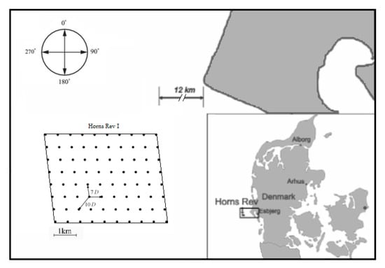
Figure 3.
Baseline layout of Horns Rev I and its location with respect to the Danish coast.
Due to its high computational cost, a fully resolved wind rose would not be feasible to be applied to each individual throughout the thousands of generations during the optimization process. Therefore, a relatively simplified (but still resolved enough) wind rose (72 directions and 1 wind speed) was applied during the evolution (WRevol, Figure 4b). In turn, the wind rose used for evaluation of the obtained solutions (WReval, Figure 4a) is fully resolved, with 120 wind directions (3 resolution) and 22 wind speeds (1 m/s resolution). WRevol was derived in such a way that the wind speeds at each sector provided the same wind power output as in WReval, which ranged between 9.9 and 8.3 m/s. The roughness lengths was set to 0.0002 (following [39,74,94]), whereas the undisturbed turbulence intensity I was set to 0.076 (following the average level for the offshore wind farm in [95]). This I value produces a near wake region of ∼2D (see [68] for details), a region not defined for the EPFL Gaussian wake model. To ensure avoiding it, a of 2.5D was imposed for this work.
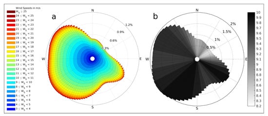
Figure 4.
Wind roses from Horns Rev used respectively for evaluation (a) and evolution (b).
2.6. Wind Farm Maximum Length Constraint
Theoretically, the unconstrained area shape MO-WFLO presents an unbounded result in the region of the PO maximization, related to a wind farm length. With no further constraint, a continuously maximized PO might lead to an infinitely long and thin wind farm area solution (hereafter called ‘long-WF’ solution). For this reason, a constraint on the maximum length of the wind farm for solutions attaining rather unpractical lengths was considered. The maximum length constraint was set to 3 times the maximum length of the benchmark case, HR, which provides a limit of 20.26 km. This distance was set as a balance between optimization flexibility on one side, and the current wind farm sizing state-of-the-art on the other. To this last extent, 20 km can be still accepted as a realistic size, as several offshore wind farms in the North Sea even exceed this length, including several ones in Denmark (e.g., Anholt [96] or Horns Rev 3 [97]). In addition to the constrained case (lC), an unconstrained maximum WF length scenario (no-lC) was also considered for comparison.
3. Results
The 13 algorithms were run on a 16-core computer cluster, each core equipped with 64 GB DDR3 RAM and 2.6 GHz. After the algorithms run, their performance was assessed and compared to the baseline case (Horns Rev I wind farm, HR) based on their objective functions (Section 3.1) and their Pareto fronts (Section 3.2). In the same section, all the Pareto fronts obtained for each algorithm are used to derive a single, aggregated Pareto front (), that depicts all the non-dominated solutions attained in this work. Finally, a utility function for a decision maker in Denmark is designed and applied to the aggregated Pareto front as an example of application following a MO optimization (Section 3.5). As a general remark, it must be pointed out that only the ‘hybrid3’ algorithm exceeded the maximum WF length constraint during its evolution, so only this algorithm presents results for both lC and no-lC cases. Results on all the other algorithms are considered to be lC results, as in practice none of their solutions exceeded the length constraint.
3.1. Maximum Power Output and Minimum Cable Length
Before addressing the Pareto fronts in general, here we analyze the results regarding the two objective functions one by one. To this regard, the followed variable-shape MO-WFLO strategy generated a wide range of solutions that remarkably increased the Power Output and decreased the Cable Length compared to the baseline Horns Rev I layout. Moreover, several of the newly developed algorithms largely outperformed NSGA-II, on either PO or CL objective functions. Overall, up to 9 of the 12 newly developed algorithms exceeded the baseline PO, in addition to the ‘hybrid3-no-lC’ version. In turn, all solutions from all 13 algorithms attained shorter Cable Length values than the baseline. In detail, the set of solutions attained by NSGA-II presented values ranging from a 0.2% PO improvement to a 61.4% CL reduction against the HR baseline (HR-b). In turn, the algorithms introduced in this work showed PO improvements up to 5.9% in the no-lC case (‘hybrid3’), and up to 2.4% in the lC case (‘hybrid6’). This last result implies an improvement 10 times bigger compared to the PO improvement attained with the fixed wind farm through the CEGA algorithm in [39], which reached a 0.24% PO increase against HR-b. Finally, regarding CL, the developed algorithms reached up to 62.1% reduction (‘V-CEGA-noHF’) against HR-b.
The way algorithms evolved through either PO or CL differed remarkably from one algorithm to another (Figure 5). Although algorithms evolving through PO rather quickly in general stagnate relatively fast (e.g., ‘hybrid4’, ‘V-CEGA-SBX’, ‘NSGA-II’), others evolving more slowly attain better final performance (e.g., ‘hybrid2’, ‘hybrid6’). These behaviors agree with a rather convergence-oriented (exploitation) and diversity-oriented (exploration) algorithms, respectively. An exception to these behaviors, with an apparently balanced evolution trade-off between diversity and convergence, would be represented by the algorithm ‘hybrid5’ (always addressing PO evolution alone), which finally attains the biggest improvement (lC case). Regarding CL-reduction evolution, differences are much smaller, improvements ranging between 60.1% and 62.1% CL-reduction. There, ‘V-CEGA-SBX’ shows a very well-balanced evolution, evolving less than many algorithms initially, although finally attaining the largest CL reduction.

Figure 5.
Evolution of the maximum PO (a) and minimum CL (b) obtained at each generation for the algorithms considered. Dashed black/orange line (a) shows the evolution of ‘hybrid3’ with no constraint.
3.2. Non-Dominated Solutions Regarding the Aggregated Pareto Front
The main goal in a multi-objective optimization is to obtain the most performing Pareto front as possible (i.e., to obtain a Pareto front as close as possible to the IOV). For this reason, the overall performance of a given MO optimization algorithm must be measured throughout the whole set of solutions forming its Pareto front. For instance, two or more MO algorithms can be compared through the relative position of their Pareto fronts [98]. On this basis, the performance of a certain amount of MO algorithms can be compared by computing the aggregated Pareto front formed by all Pareto fronts produced by each algorithm individually, and then measuring the contribution to that aggregated front by each algorithm. In this work we have derived this contribution by calculating the ratio of the aggregated front length produced by each algorithm. This has been done as follows:
- (1)
- First, the aggregated Pareto front is computed (i.e., the solutions forming the aggregated Pareto front are selected).
- (2)
- Next, the midpoints of the segments formed by all solutions two by two are calculated.
- (3)
- Then, a score is provided to each solution, equal to the length between its two surrounding midpoints. As vertices and are surrounded by only one midpoint, they receive a score equal to the distance to it.
- (4)
- The final score of as given algorithm is the sum of the scores associated with its solutions, divided by the whole length of the aggregated front.
The relative performance of each algorithm was computed according to the aggregated Pareto front ratio () for the whole evolution. Figure 6 shows in terms of % of the whole aggregated Pareto front at each time step, for both unconstrained (a) and constrained (b) maximum wind farm length cases. Results show that up to the first 20% of the simulation, ‘hybrid5’ clearly leads the evolution, gartering up to 75% of the aggregated Pareto front. Then, for the unconstrained maximum WF length case, its prevalence is sharply and completely substituted by ‘hybrid3’, which joins the long-WF region and takes the lead clearly exceeding all the rest of algorithms until the end of the evolution. On the constrained maximum WF length case, this substitution also happens, but it is gradual and partial, this in some degree produced by the length limitation of ‘hybrid3’. This allows the irruption of other algorithms as ‘hybrid2’, and in part also ‘V-CEGA-PMUT’ towards the end of the evolution.
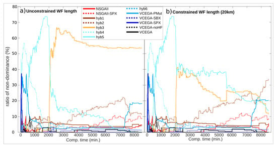
Figure 6.
Temporal evolution of the non-dominance ratio by each algorithm during the optimization, for the cases without (a) and with (b) max. WF length constraint. Non-dominance is computed considering the aggregated Pareto front formed by all algorithm solutions at each time step. The algorithm ‘hybrid5’ holds most of the aggregated Pareto front up to the first 36 h of simulation, whereas ‘hybrid3’ and ‘hybrid2’ finally obtain the lead.
Figure 7 depicts the final aggregated Pareto front on the objective space at the end of the simulation (), for both lC and no-lC cases. ‘hybrid3’ gathers more than half of the front, clearly dominating the region of the PO objective function when no maximum length constraint is applied, whereas it is substituted by ‘hybrid2’ and ‘hybrid5’ (attaining a remarkably smaller PO) when it is indeed applied. ‘hybrid2’ (and still partly ‘hybrid3’) dominate the central zone of the , whereas ‘V-CEGA-PMUT’ gathers most of the CL-reduction region (although the absolute minimum CL is attained with ‘V-CEGA-SBX’).
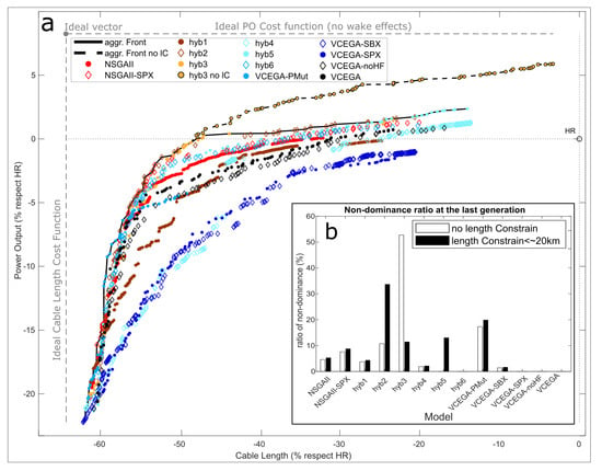
Figure 7.
(a) Pareto fronts obtained from each algorithm at the final generation (see legend for color codes), and aggregated Pareto front applying (solid black line) and not applying (dashed black line) a maximum wind farm length constraint. (b) Ratio of non-dominance of each algorithm at the final generation, for both the constrained and unconstrained maximum wind farm length cases. Results highlight the largest role by the algorithm ‘hybrid3’ in the Aggregated Pareto front at the end of the run when no constrain is applied, and by ‘hybrid2’ when it is applied.
The attained aggregated Pareto front shows that the set of algorithms designed for this work operate in a complementary manner. At the same time, it can be noted that a major part of the can be represented by only a few of the considered algorithms. For instance, in the no-lC case, an approach with ‘hybrid3’ (especially on the PO region) and ‘V-CEGA-PMUT’ (especially on the CL region) alone can generate a well-balanced Pareto front, very near the and covering more than 70% of it. In turn, for the lC case the considered algorithms work more complementary, and some more algorithms are recommended to be considered. Essentially, ‘hybrid2’ and ‘hybrid5’ would cover most of the PO region, whereas ‘V-CEGA-PMUT’ and ‘hybrid3’ would cover a large section of the CL and the PO-CL transition region, respectively. These 4 algorithms cover 78% of (>66% without ‘hybrid3’). It must be pointed out, though, that these selections (lC and no-lC cases) would not cover the minimum CL (provided by ‘V-CEGA-SBX’) solution (although a solution with just 260 m more CL would be included).
3.3. Performance Comparison of the Applied Algorithms
Beyond highlighting the algorithms with a biggest role on the (and thus best suitable for VariShape MO-WFLO), comparing algorithms two by two can provide some clues on their suitability. For instance, NSGA-II (red circles) is clearly outperformed by NSGA-SPX (red diamonds) throughout the whole range of non-dominated solutions. This demonstrates that overall, SBX is indeed not the most appropriate crossover strategy for the VariShape MO-WFLO problem. Instead, SBX only appears to be partly useful in two very specific circumstances. First, it seems to operate correctly in the extreme CL-reduction region (via ‘V-CEGA-SBX’), where distances between turbines are so small that its big associated diversity strength can find optimum solutions more easily than others, without excessively distorting the layouts of the offspring individuals. Secondly, it seems to provide some useful results within ‘hybrid3’, where, with no maximum length constraint, its high diversity potential seems to favor the layout elongation rather faster than the rest of algorithms.
Regarding the slight variations on V-CEGA, it is proven that using a reservoir that keeps previous non-dominated solutions and reintroduces them along further generations results in an appropriate strategy, ‘V-CEGA’ outperforming ‘V-CEGA-noHF’ throughout all the Pareto fronts. Overall, it is shown that the slight variations on V-CEGA regarding crossover (‘V-CEGA-SBX’, ‘V-CEGA-SPX’) fail to improve the CEGA crossover in V-CEGA, whereas only a combination of CEGA crossover and polynomial mutation (‘V-CEGA-PMUT’) provides partly a successful outcome (over the CL region).
Regarding the hybridized versions and their three characterizing features (breeding, selection and structure), it is worth highlighting that the V-CEGA breeding, through its presence in ‘hybrid2’ and ‘hybrid5’, holds the best performance overall when the problem is constrained with a realistic maximum WF length, covering most of the including all the PO region. This seems to work particularly well with NSGA-II selection, as both hybrids hold it, showing that V-CEGA selection is an element that does not seem highly efficient when taken outside the full V-CEGA algorithm (as it happens in hybrids 1 and 4). Interestingly, comparing NSGA-II and V-CEGA alone shows that they complement intermittently through their aggregated Pareto front, NSGA-II holding though the central part of the front, and V-CEGA rather through most of the CL and PO regions. This demonstrates the value of having designed new hybrid algorithms that, when combined, outperformed both original ones.
3.4. Results of the Aggregated Pareto Pront
When having an overall look to the whole , a rather balanced outcome is obtained for the no-lC case, with a rather progressive transition from the CL to the PO-dominant objective function regions, a symptom of having addressed the VariShape MO-WFLO problem in a balanced manner. This progressive transition is partially broken when the maximum length constraint is applied, this revealing a prohibited region in the objective space just after exceeding the baseline PO level. Despite that, it can be highlighted that within the lC case, the solutions are still able to further progress through the PO region (although in a more flattened manner) up to a PO level 2.4% higher than HR-b (‘hybrid5’).
Figure 8 depicts the wind farm solutions corresponding to the (selection). For practical reasons, one every two solutions are represented on the lC case (including and ), plus a selection of five ‘hybrid3’ solutions from the no-lC version. As it can be observed, a progressive transition becomes clear, from very concentrated layouts (with a bigger performance in CLs) to more expanded ones (similar to those attained in [13]), until reaching significantly elongated shapes (with bigger performance in PO). Interestingly, results within the constrained length case also show that the relative minimum width of the solutions throughout ends up by increasing again as they approach the region with highest PO values, an outcome that is subject of further investigation. It is shown that solutions produced by algorithm ‘hybrid3’ (no-lC case) allow this algorithm to obtain the highest PO values, but with the drawback of having very long wind farm lengths (>40 km). On the other hand, when the maximum WF length constraint is applied, most of these solutions are removed from the , and the maximum PO is provided by several solutions belonging to ‘hybrid5’ with a wider shape and remarkably more moderate lengths (∼17 km).
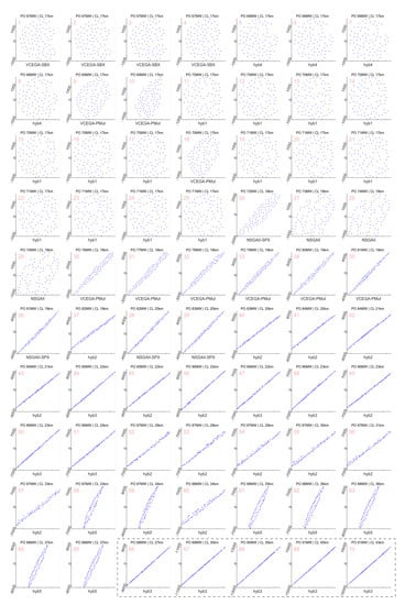
Figure 8.
Set of obtained solutions (wind farm layouts) throughout the obtained aggregated Pareto front in the final generation. Top labels at each solution show the PO and CL values obtained, while bottom labels indicate the algorithm producing it. Solutions are sorted from minimum CL (top left) to maximum PO (down right), following the aggregated Pareto front (black line at Figure 7). The dashed square marks out a selection of the solutions exclusively obtained with no maximum WF length constrain.
3.5. Decision Maker in Denmark
A decision maker (DM) is a human [81] or artificial [99] entity in charge to make a choice for a final solution out from the set of solutions provided by the MO optimization. The DM carries out its choice relying on a utility function, which characterizes the set of solutions according to some particularized criteria that responds to its own needs [81]. In this work we have modeled a utility function for a DM localized in Denmark and have applied it to the obtained solutions, to provide an example of a DM selection of a single final solution.
The levelized cost of energy (LCOE) based on the local conditions in Denmark was established here as the DM utility function. LCOE is a widely employed economic indicator that measures the relationship between the lifetime costs of a power-generating asset with respect to its lifetime energy production. In this work we have followed the LCOE used in [100] and other offshore wind power works [101]:
where , , and are respectively the investment cost, the operation and maintenance cost, the fuel cost and the produced energy at year y, whereas r is the discount rate, throughout a lifespan period of 25 years. Naturally, here = 0. Details on the expressions for , and can be found in Appendix A.
The obtained LCOE values for the ranged between 0.0654 EUR/kWh and 0.0505 EUR/kWh (lC) or 0.0489 EUR/kWh (no-lC). These values are in line with other LCOE estimates for offshore wind power [102,103]. The two latter values (minimum LOCEs) represent 2.7% (lC) and 5.7% (no-lC) LCOE reduction with respect to the baseline LCOE (0.0519 EUR/kWh). Figure 9 shows some relevant examples of solutions (expanded from Figure 8) corresponding with the LCOE extremes obtained. In addition, the solution showing the maximum possible CL reduction while obtaining a PO similar to the baseline is also depicted (Figure 9b).
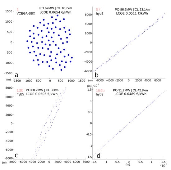
Figure 9.
Samples of solutions throughout the obtained aggregated Pareto front in the final generation () holding LCOE extremes obtained for a decision maker in Denmark: (a) max. LCOE (and minimum Cable Length), (b) similar PO as baseline, (c) min. LCOE (and max. PO) with max. WF length constraint and (d) min. LCOE (and max. PO) without max. WF length constraint. Numbers in pink stand for its sorting positions in the (from min. CL to max PO). Circles represent the turbine rotors proportional to their relative size.
Considering the particularities of the utility function employed, it can be observed that minimum LCOEs are obtained for those solutions providing the highest POs, for both no-lC or lC cases. Comparing the two initial objective functions (CL and PO) with the derived utility function LCOE for the whole set of solutions, some relationships can be highlighted. Figure 10 shows LCOE plot-scattered against PO and CL for these solutions. CL is shown to be strongly inversely related to LCOE for small CL values, whereas it becomes nearly unrelated to it for the biggest CL lengths (from ∼25 km). In turn, PO appears directly related to LCOE for all PO values, although this relationship starts stagnating for big PO values (for both lC and no-lC cases). Overall, for the particular features defining the derived LCOE (cable price, turbine cost, etc.), the set of solutions shows not having reached an absolute minimum LCOE value, and suggest smaller LCOE values could be reached with bigger PO solutions. However, this does not prevent from the fact that if other values of the utility function are used (e.g., a more expensive cable price), an absolute minimum LCOE may be attained for the obtained set of solutions.
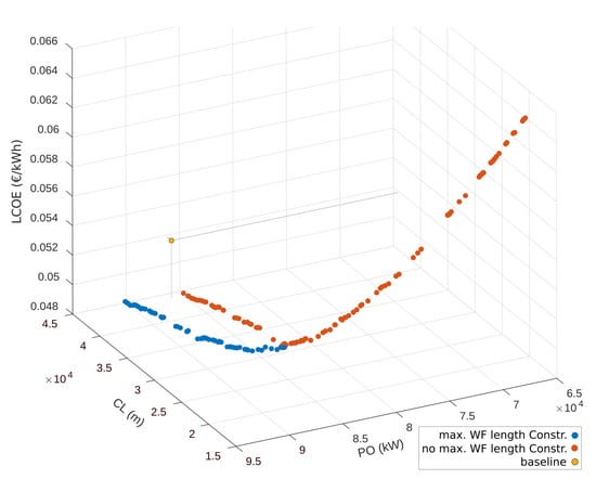
Figure 10.
LCOE particularized for a decision maker in Denmark compared to PO and CL, for the set of solutions and the baseline solution (yellow dot). lC (no-lC) solutions are represented with orange (blue) dots.
4. Conclusions
In this work we have carried out the optimization of the wind farm area shape using multi-objective (MO) optimization on 13 different genetic algorithms. These included a novel algorithm for wind farm layout MO, a traditionally used MO algorithm (NSGA-II), and 11 hybridized versions combining elements from the two. The objective functions considered were the overall power output (PO) and the electricity cable length (CL), which were evaluated through the EPFL Gaussian analytical wake model [68,74] and the minimum spanning tree function [84], respectively. Finally, an expression for the levelized cost of energy was derived and applied to the obtained solutions in the Pareto Front.
Providing total freedom to the area shape during the optimization has shown high added value to the WFLO problem, especially taking into account that the total surface (amount of km) was always kept below or equal to the baseline case (Horns Rev I, Denmark). Results showed a power output improvement compared to the baseline up to 10 times larger (2.4%) than the attained through single-objective WFLO [39] with fixed area (0.24%). These results were attained by imposing a constraint (lC) to the maximum wind farm length (∼20 km, 3 times the maximum Horns Rev I length). Aside, a length-unconstrained case (no-lC) provided improvements up to 5.9%. These results were obtained through two newly developed MO algorithms, product of the hybridization between V-CEGA (a MO-adaption of the CEGA algorithm [39]) and the traditionally used NSGA-II [69] MO algorithm. The Pareto front resulting from aggregating the individual Pareto fronts from the 13 algorithms provided solutions ranging from 62.1% CL reduction (but 22% smaller PO) to 2.4% (5.9%) PO improvement and 14% (3.3%) CL reduction for the constrained (unconstrained) maximum length. The solution holding a similar baseline PO provided a 14% CL reduction.
Although NSGA-II or V-CEGA alone did not show low performance overall, they were outperformed by non-dominated solutions from hybridized algorithms throughout ∼95% of the aggregated front (either through lC or no-lC), which supports a hybridization-based algorithm design strategy. Although the different algorithms provided complementary solutions, results showed that just three (two) algorithms were enough to cover 66% (70%) of the lC (no-lC) aggregated front, and included most of the relevant solutions attained. In this way, the variable area shape MO-WFLO problem with lC (no-lC) showed highest efficiency through ‘hybrid2’, ‘V-CEGA-PMUT’ and ‘hybrid5’ (‘hybrid3’ and ‘V-CEGA-PMUT’) algorithms (see algorithms description, Section 2.4).
In the performance of the algorithm operators, results indicate that simulated binary crossover SBX (used e.g., in NSGA-II) is not the most appropriate crossover for the MO-WFLO problem addressed. This can be explained as WFLO, in general, is highly sensitive to the relative variation of the turbine positions due to their associated strong effect on wake induced power losses, a relative positioning that is highly disrupted with the halfway positioning scheme applied in the SBX crossover. This contrasts with other crossovers as CEGA (or to a smaller extent SPX), in which the relative positions among turbines is modified in a smoother way. In turn, the vertex-based selection method seems to be only efficient when hybridized in combination with the V-CEGA structure.
Multi-Objective optimization allowed to derive a wide range of solutions, progressively transiting from strongly compacted, rounded wind farms (in the minimum CL region), to very elongated ones with ∼17 km (>40 km) length within the lC (no-lC) case (in the maximum PO region), or to more CL-PO optimization-balanced solutions. The choice on the final solution is left to the decision maker (e.g., wind farm managers) according to its particular needs. In this work, a case-study utility function based on the levelized cost of energy (LCOE) was derived for a potential decision maker located in Denmark, for all solutions located in the obtained aggregated Pareto front. Results showed that the proposed MO-WFLO methodology is capable of providing 2.7% (5.7%) smaller LCOEs within the lC (no-lC) case compared to the baseline value (0.0519 EUR/kWh), and indicate that the optimum LCOE values for the particular economic parameters considered fall around the maximum PO area of the objective space.
Author Contributions
Conceptualization, N.K.-B. and F.P.-A.; methodology, N.K.-B. and F.P.-A.; formal analysis, N.K.-B. and F.P.-A.; investigation, N.K.-B. and F.P.-A.; software, N.K.-B.; resources, F.P.-A.; data curation, N.K.-B.; validation, N.K.-B.; visualization, N.K.-B.; writing—original draft preparation, N.K.-B. and F.P.-A.; writing—review and editing, N.K.-B. and F.P.-A.; supervision, F.P.-A.; project administration, F.P.-A.; funding acquisition, F.P.-A. All authors have read and agreed to the published version of the manuscript.
Funding
This research was supported by the Swiss Federal Office of Energy (Grant SI/502135-01) and the Swiss Centre for Competence in Energy Research on the Future Swiss Electrical Infrastructure (SCCER-FURIES) with the financial support of the Swiss Innovation Agency (Innosuisse—SCCER program, contract Number 1155002544).
Institutional Review Board Statement
Not applicable.
Informed Consent Statement
Not applicable.
Data Availability Statement
The Horns Rev wind rose was adapted from [104].
Conflicts of Interest
The authors declare no conflict of interest.
Abbreviations
| maximum area of the wind farm | |
| area of the wind farm | |
| CEGA | crossover-elitist genetic algorithm |
| CL | cable length |
| export cable length | |
| substation cable length | |
| thrust coefficient | |
| cost of cable installation | |
| wind farm investment cost in year y | |
| wind farm operations and maintenance costs in year y | |
| wind turbine cost | |
| D | turbine rotor diameter |
| d, | distance to IOV, normalized distance to IOV |
| DM | decision maker |
| initial wake expansion parameter | |
| crossover distribution index for NSGA-II | |
| mutation distribution index for NSGA-II | |
| Energy produced in year y | |
| EPFL | École Polytechnique Fédéral de Lausanne |
| objective function | |
| F(x) | solution in the objective space |
| Pareto front | |
| aggregated Pareto front | |
| generation gap | |
| HR | Horns Rev I wind farm |
| HR-b | baseline layout of the Horns Rev I wind farm |
| I | turbulence intensity level |
| IOV | ideal objective vector |
| wake growth rate | |
| objective space | |
| L | electricity cable transport losses |
| lC | constrained maximum wind farm length |
| LCOE | levelized cost of energy |
| LES | large eddy simulation |
| M | number of objective functions |
| optimum ideal value of the objective function | |
| MO | multi-objective |
| MOEA | multi-objective evolutionary algorithm |
| N | number of individuals in the population |
| number of individuals in the selected population | |
| NSGA-II | Non-dominated Sorting Genetic Algorithm version II |
| decision space | |
| crossover operator in CEGA and V-CEGA | |
| crossover probability in NSGA-II | |
| mutation probability in NSGA-II | |
| mutation operator in CEGA, V-CEGA | |
| electricity cable price | |
| PO | power output |
| power output at turbine t, angular sector s and velocity bin b | |
| PMUT | polynomial mutation |
| random number | |
| aggregated Pareto front ratio | |
| r | discount rate |
| S | offshore substation |
| size of the Pareto front | |
| SBX | simulated binary crossover |
| SPX | single point crossover |
| T | number of turbines |
| uniform distribution | |
| streamwise incoming velocity | |
| streamwise incoming velocity in turbine j | |
| streamwise incoming velocity in turbine j produced by wake in turbine i | |
| streamwise velocity deficit | |
| V, | Pareto front vertex, normalized Pareto front vertex |
| V-CEGA | vertex crossover-elitist genetic algorithm |
| WFLO | wind farm layout optimization |
| WF | wind farm |
| streamwise, spanwise and vertical coordinates in the wind farm | |
| non-dominated solution in the decision space | |
| dominated solution in the decision space | |
| X | Euclidean distance in the wind farm |
| wind farm lifespan | |
| turbine hub height |
Appendix A
In this appendix, the values for , , and r used in this work that take part of the LCOE definition,
are briefly described:
: In this study, we consider that all the investment is done during the first year, so if y ≠ 1, then = 0. HR investment costs were summarized into the V-80 turbines cost, the substation cost and cost of the three different electricity cables involved. First, according to details in [105], to each turbine (installation included) a cost of 4 M€ was assigned. The substation S, according to its features, with a transformer station (34 kV to 170 kV) and a heliport, received an estimated cost of 2.2 million EUR according to data from [106] (installation included). Then, three different electricity cable types were considered. First, the array cable interconnects the turbines inside the wind farm (variable for each solution, and represented by CL). For HR, CL was found to be a 100 mm thickness cable [107]. This equals to a 240 mm cable standard [108], which has a price of = 253 EUR/m [109]. Then, the substation cable connects the turbines with the substation. It consists of a 34 kV 130 mm thick cable [107], which stands for a 400 mm cable standard [108], with a price of 340 EUR/m [109]. This cable length was set constant (20 km). Finally, the export cable , which connects the substation and the shore (21 km [108]), is a 630 mm cable [108], which has a price of 675 EUR/m [65]. The cables installation cost was set to 260 EUR/m [110] for all cable types. With all this, can be defined as:
: , which is equal to the annual energy produced (AEP), is the result of multiplying the power output PO by the number of hours a year, 8760, minus the energy losses experienced throughout all the different type of cables. The ratio of energy losses can be computed as follows:
where , and are the losses within the array cable, the substation cable and the export cable, respectively. , and have a tabulated value of 6% loss every 1000 km [111], 5% loss every 1000 km [111] and 1.55% loss every 50 km [112]. With this, can be defined as:
so that
: Maintenance and operation costs per kWh were set to 0.03 EUR/kWh as a midpoint between the range of 0.015–0.045 EUR/kWh [113], so it can be given by this expression:
r: Finally, the discount rate r for an unlevered offshore wind company in Denmark was found to be 7% (“Nordics” in [114]).
References
- Alfredsson, P.H.; Dahlberg, J.A. Measurements of wake interaction effects on the power output from small wind turbine models. NASA STI/Recon Tech. Rep. N 1981, 82, 18720. [Google Scholar]
- Barthelmie, R.J.; Hansen, K.; Frandsen, S.T.; Rathmann, O.; Schepers, J.; Schlez, W.; Phillips, J.; Rados, K.; Zervos, A.; Politis, E.; et al. Modelling and measuring flow and wind turbine wakes in large wind farms offshore. Wind Energy Int. J. Prog. Appl. Wind Power Convers. Technol. 2009, 12, 431–444. [Google Scholar] [CrossRef]
- Porté-Agel, F.; Bastankhah, M.; Shamsoddin, S. Wind-turbine and wind-farm flows: A review. Bound. Layer Meteorol. 2020, 174, 1–59. [Google Scholar] [CrossRef] [PubMed] [Green Version]
- Porté-Agel, F.; Wu, Y.T.; Chen, C.H. A numerical study of the effects of wind direction on turbine wakes and power losses in a large wind farm. Energies 2013, 6, 5297–5313. [Google Scholar] [CrossRef]
- Herbert-Acero, J.F.; Probst, O.; Réthoré, P.E.; Larsen, G.C.; Castillo-Villar, K.K. A review of methodological approaches for the design and optimization of wind farms. Energies 2014, 7, 6930–7016. [Google Scholar] [CrossRef]
- Poku, M.Y.B.; Biegler, L.T.; Kelly, J.D. Nonlinear optimization with many degrees of freedom in process engineering. Ind. Eng. Chem. Res. 2004, 43, 6803–6812. [Google Scholar] [CrossRef]
- Frandi, E.; Papini, A. Coordinate search algorithms in multilevel optimization. Optim. Methods Softw. 2014, 29, 1020–1041. [Google Scholar] [CrossRef]
- Etemaadi, R.; Chaudron, M.R. New degrees of freedom in metaheuristic optimization of component-based systems architecture: Architecture topology and load balancing. Sci. Comput. Program. 2015, 97, 366–380. [Google Scholar] [CrossRef]
- Chen, K.; Song, M.; He, Z.; Zhang, X. Wind turbine positioning optimization of wind farm using greedy algorithm. J. Renew. Sustain. Energy 2013, 5, 023128. [Google Scholar] [CrossRef]
- Chen, K.; Song, M.; Zhang, X.; Wang, S. Wind turbine layout optimization with multiple hub height wind turbines using greedy algorithm. Renew. Energy 2016, 96, 676–686. [Google Scholar] [CrossRef]
- Stanley, A.P.; Thomas, J.; Ning, A.; Annoni, J.; Dykes, K.; Fleming, P.A. Gradient-Based Optimization of Wind Farms with Different Turbine Heights. In Proceedings of the 35th Wind Energy Symposium, Grapevine, TX, USA, 9–13 January 2017; p. 1619. [Google Scholar]
- Stanley, A.P.; Ning, A. Coupled wind turbine design and layout optimization with nonhomogeneous wind turbines. Wind Energy Sci. 2019, 4, 99–114. [Google Scholar] [CrossRef] [Green Version]
- Wu, C.; Yang, X.; Zhu, Y. On the design of potential turbine positions for physics-informed optimization of wind farm layout. Renew. Energy 2021, 164, 1108–1120. [Google Scholar] [CrossRef]
- Hou, P.; Zhu, J.; Ma, K.; Yang, G.; Hu, W.; Chen, Z. A review of offshore wind farm layout optimization and electrical system design methods. J. Mod. Power Syst. Clean Energy 2019, 7, 975–986. [Google Scholar] [CrossRef] [Green Version]
- Grilli, A.; Spaulding, M.; O’Reilly, C.; Potty, G. Offshore wind farm Macro and Micro siting protocol Application to Rhode Island. Coast. Eng. 2012, 2. [Google Scholar] [CrossRef] [Green Version]
- Liu, F.; Ju, X.; Wang, N.; Wang, L.; Lee, W.J. Wind farm macro-siting optimization with insightful bi-criteria identification and relocation mechanism in genetic algorithm. Energy Convers. Manag. 2020, 217, 112964. [Google Scholar] [CrossRef]
- Li, W.; Özcan, E.; John, R. Multi-objective evolutionary algorithms and hyper-heuristics for wind farm layout optimisation. Renew. Energy 2017, 105, 473–482. [Google Scholar] [CrossRef] [Green Version]
- Guirguis, D.; Romero, D.A.; Amon, C.H. Gradient-based multidisciplinary design of wind farms with continuous-variable formulations. Appl. Energy 2017, 197, 279–291. [Google Scholar] [CrossRef]
- Tong, W.; Chowdhury, S.; Mehmani, A.; Messac, A.; Zhang, J. Sensitivity of wind farm output to wind conditions, land configuration, and installed capacity, under different wake models. J. Mech. Des. 2015, 137, 061403. [Google Scholar] [CrossRef]
- Ching-Lai, H.; Abu, S.M.M. Multiple Objective Decision Making, Methods and Applications: A State-of-the-Art Survey; Springer: Berlin/Heidelberg, Germany, 1979. [Google Scholar]
- Sawaragi, Y.; Nakayama, H.; Tanino, T. Theory of Multiobjective Optimization; Elsevier: Amsterdam, The Netherlands, 1985; Volume 176. [Google Scholar]
- Coello, C.A.C. A comprehensive survey of evolutionary-based multiobjective optimization techniques. Knowl. Inf. Syst. 1999, 1, 269–308. [Google Scholar] [CrossRef]
- Anvari-Moghaddam, A.; Monsef, H.; Rahimi-Kian, A. Cost-effective and comfort-aware residential energy management under different pricing schemes and weather conditions. Energy Build. 2015, 86, 782–793. [Google Scholar] [CrossRef]
- Kim, J.; Moon, I. Strategic design of hydrogen infrastructure considering cost and safety using multiobjective optimization. Int. J. Hydrog. Energy 2008, 33, 5887–5896. [Google Scholar] [CrossRef]
- Ascione, F.; Bianco, N.; De Stasio, C.; Mauro, G.M.; Vanoli, G.P. A new methodology for cost-optimal analysis by means of the multi-objective optimization of building energy performance. Energy Build. 2015, 88, 78–90. [Google Scholar] [CrossRef]
- Abido, M.A. Environmental/economic power dispatch using multiobjective evolutionary algorithms. In Proceedings of the 2003 IEEE Power Engineering Society General Meeting (IEEE Cat. No. 03CH37491), Toronto, ON, Canada, 13–17 July 2003; Volume 2, pp. 920–925. [Google Scholar]
- Oliveira, C.; Antunes, C.H. A multiple objective model to deal with economy–energy–environment interactions. Eur. J. Oper. Res. 2004, 153, 370–385. [Google Scholar] [CrossRef]
- Zakariazadeh, A.; Jadid, S.; Siano, P. Economic-environmental energy and reserve scheduling of smart distribution systems: A multiobjective mathematical programming approach. Energy Convers. Manag. 2014, 78, 151–164. [Google Scholar] [CrossRef]
- Zhu, Y.; Wang, J.; Qu, B. Multi-objective economic emission dispatch considering wind power using evolutionary algorithm based on decomposition. Int. J. Electr. Power Energy Syst. 2014, 63, 434–445. [Google Scholar] [CrossRef]
- Abdollahzadeh, H.; Atashgar, K.; Abbasi, M. Multi-objective opportunistic maintenance optimization of a wind farm considering limited number of maintenance groups. Renew. Energy 2016, 88, 247–261. [Google Scholar] [CrossRef]
- Qu, B.; Liang, J.J.; Zhu, Y.; Wang, Z.; Suganthan, P.N. Economic emission dispatch problems with stochastic wind power using summation based multi-objective evolutionary algorithm. Inf. Sci. 2016, 351, 48–66. [Google Scholar] [CrossRef]
- Coello, C.A.C. Evolutionary multi-objective optimization and its use in finance. In Handbook of Research on Nature Inspired Computing for Economy and Management; Idea Group Publishing: Hershey, PA, USA, 2006. [Google Scholar]
- Ravi, V.; Pradeepkumar, D.; Deb, K. Financial time series prediction using hybrids of chaos theory, multi-layer perceptron and multi-objective evolutionary algorithms. Swarm Evol. Comput. 2017, 36, 136–149. [Google Scholar] [CrossRef]
- Gambier, A.; Badreddin, E. Multi-objective optimal control: An overview. In Proceedings of the 2007 IEEE International Conference on Control Applications, Singapore, 1–3 October 2007; pp. 170–175. [Google Scholar]
- Logist, F.; Houska, B.; Diehl, M.; Van Impe, J.F. Robust multi-objective optimal control of uncertain (bio) chemical processes. Chem. Eng. Sci. 2011, 66, 4670–4682. [Google Scholar] [CrossRef]
- Nastasi, G.; Colla, V.; Cateni, S.; Campigli, S. Implementation and comparison of algorithms for multi-objective optimization based on genetic algorithms applied to the management of an automated warehouse. J. Intell. Manuf. 2018, 29, 1545–1557. [Google Scholar] [CrossRef]
- Yao, L.; Huang, J.H. Multi-objective optimization of energy saving control for air conditioning system in data center. Energies 2019, 12, 1474. [Google Scholar] [CrossRef] [Green Version]
- DuPont, B.; Cagan, J. A hybrid extended pattern search/genetic algorithm for multi-stage wind farm optimization. Optim. Eng. 2016, 17, 77–103. [Google Scholar] [CrossRef]
- Kirchner-Bossi, N.; Porté-Agel, F. Realistic wind farm layout optimization through genetic algorithms using a Gaussian wake model. Energies 2018, 11, 3268. [Google Scholar] [CrossRef] [Green Version]
- Yin Kwong, W.; Yun Zhang, P.; Romero, D.; Moran, J.; Morgenroth, M.; Amon, C. Multi-objective wind farm layout optimization considering energy generation and noise propagation with NSGA-II. J. Mech. Des. 2014, 136, 091010. [Google Scholar] [CrossRef]
- Sorkhabi, S.Y.D.; Romero, D.A.; Beck, J.C.; Amon, C.H. Constrained multi-objective wind farm layout optimization: Novel constraint handling approach based on constraint programming. Renew. Energy 2018, 126, 341–353. [Google Scholar] [CrossRef]
- Mittal, P.; Mitra, K.; Kulkarni, K. Optimizing the number and locations of turbines in a wind farm addressing energy-noise trade-off: A hybrid approach. Energy Convers. Manag. 2017, 132, 147–160. [Google Scholar] [CrossRef]
- Kusiak, A.; Song, Z. Design of wind farm layout for maximum wind energy capture. Renew. Energy 2010, 35, 685–694. [Google Scholar] [CrossRef]
- Şişbot, S.; Turgut, Ö.; Tunç, M.; Çamdalı, Ü. Optimal positioning of wind turbines on Gökçeada using multi-objective genetic algorithm. Wind Energy Int. J. Prog. Appl. Wind Power Convers. Technol. 2010, 13, 297–306. [Google Scholar]
- Veeramachaneni, K.; Wagner, M.; O’Reilly, U.M.; Neumann, F. Optimizing energy output and layout costs for large wind farms using particle swarm optimization. In Proceedings of the 2012 IEEE Congress on Evolutionary Computation, Brisbane, QLD, Australia, 10–15 June 2012; pp. 1–7. [Google Scholar]
- Chen, Y.; Li, H.; He, B.; Wang, P.; Jin, K. Multi-objective genetic algorithm based innovative wind farm layout optimization method. Energy Convers. Manag. 2015, 105, 1318–1327. [Google Scholar] [CrossRef]
- Rodrigues, S.; Bauer, P.; Bosman, P.A. Multi-objective optimization of wind farm layouts–Complexity, constraint handling and scalability. Renew. Sustain. Energy Rev. 2016, 65, 587–609. [Google Scholar] [CrossRef] [Green Version]
- Tran, R.; Wu, J.; Denison, C.; Ackling, T.; Wagner, M.; Neumann, F. Fast and effective multi-objective optimisation of wind turbine placement. In Proceedings of the 15th Annual Conference on Genetic and Evolutionary Computation, Amsterdam, The Netherlands, 6–10 June 2013. [Google Scholar]
- Feng, J.; Shen, W.Z.; Xu, C. Multi-Objective Random Search Algorithm for Simultaneously Optimizing Wind Farm Layout and Number of Turbines; Journal of Physics: Conference Series; IOP Publishing: Bristol, UK, 2016; Volume 753, p. 032011. [Google Scholar]
- Mustakerov, I.; Borissova, D. Wind park layout design using combinatorial optimization. In Wind Turbines; IntechOpen: Rijeka, Croatia, 2011; pp. 403–424. [Google Scholar]
- Turner, S.; Romero, D.; Zhang, P.; Amon, C.; Chan, T. A new mathematical programming approach to optimize wind farm layouts. Renew. Energy 2014, 63, 674–680. [Google Scholar] [CrossRef]
- MirHassani, S.; Yarahmadi, A. Wind farm layout optimization under uncertainty. Renew. Energy 2017, 107, 288–297. [Google Scholar] [CrossRef]
- Fleming, P.A.; Ning, A.; Gebraad, P.M.; Dykes, K. Wind plant system engineering through optimization of layout and yaw control. Wind Energy 2016, 19, 329–344. [Google Scholar] [CrossRef] [Green Version]
- Eroğlu, Y.; Seçkiner, S.U. Design of wind farm layout using ant colony algorithm. Renew. Energy 2012, 44, 53–62. [Google Scholar] [CrossRef]
- Chowdhury, S.; Zhang, J.; Messac, A.; Castillo, L. Unrestricted wind farm layout optimization (UWFLO): Investigating key factors influencing the maximum power generation. Renew. Energy 2012, 38, 16–30. [Google Scholar] [CrossRef]
- Pookpunt, S.; Ongsakul, W. Optimal placement of wind turbines within wind farm using binary particle swarm optimization with time-varying acceleration coefficients. Renew. Energy 2013, 55, 266–276. [Google Scholar] [CrossRef]
- Rahmani, R.; Khairuddin, A.; Cherati, S.M.; Pesaran, H.M. A novel method for optimal placing wind turbines in a wind farm using particle swarm optimization (PSO). In Proceedings of the IPEC, IEEE 2010 Conference Proceedings, Singapore, 27–29 October 2010; pp. 134–139. [Google Scholar]
- Mosetti, G.; Poloni, C.; Diviacco, B. Optimization of wind turbine positioning in large windfarms by means of a genetic algorithm. J. Wind Eng. Ind. Aerodyn. 1994, 51, 105–116. [Google Scholar] [CrossRef]
- Salcedo-Sanz, S.; Gallo-Marazuela, D.; Pastor-Sánchez, A.; Carro-Calvo, L.; Portilla-Figueras, A.; Prieto, L. Evolutionary computation approaches for real offshore wind farm layout: A case study in northern Europe. Expert Syst. Appl. 2013, 40, 6292–6297. [Google Scholar] [CrossRef]
- Salcedo-Sanz, S.; Gallo-Marazuela, D.; Pastor-Sánchez, A.; Carro-Calvo, L.; Portilla-Figueras, A.; Prieto, L. Offshore wind farm design with the Coral Reefs Optimization algorithm. Renew. Energy 2014, 63, 109–115. [Google Scholar] [CrossRef]
- Bilbao, M.; Alba, E. CHC and SA applied to wind energy optimization using real data. In Proceedings of the Evolutionary Computation (CEC), 2010 IEEE Congress on Evolutionary Computation, Barcelona, Spain, 18–23 July 2010; pp. 1–8. [Google Scholar]
- Huang, H.S. Distributed genetic algorithm for optimization of wind farm annual profits. In Proceedings of the 2007 International Conference on Intelligent Systems Applications to Power Systems, Kaohsiung, Taiwan, 5–8 November 2007; pp. 1–6. [Google Scholar]
- Liu, F.; Wang, Z. Offshore wind farm layout optimization using adapted genetic algorithm: A different perspective. arXiv 2014, arXiv:1403.7178. [Google Scholar]
- Gao, X.; Yang, H.; Lu, L. Investigation into the optimal wind turbine layout patterns for a Hong Kong offshore wind farm. Energy 2014, 73, 430–442. [Google Scholar] [CrossRef]
- Réthoré, P.E.; Fuglsang, P.; Larsen, G.C.; Buhl, T.; Larsen, T.J.; Madsen, H.A. TOPFARM: Multi-fidelity optimization of wind farms. Wind Energy 2014, 17, 1797–1816. [Google Scholar] [CrossRef] [Green Version]
- Jensen, N.O. A Note on Wind Generator interaction 1983. Available online: https://backend.orbit.dtu.dk/ws/portalfiles/portal/55857682/ris_m_2411.pdf (accessed on 7 July 2021).
- Frandsen, S.; Barthelmie, R.; Pryor, S.; Rathmann, O.; Larsen, S.; Højstrup, J.; Thøgersen, M. Analytical modelling of wind speed deficit in large offshore wind farms. Wind Energy Int. J. Prog. Appl. Wind Power Convers. Technol. 2006, 9, 39–53. [Google Scholar] [CrossRef]
- Bastankhah, M.; Porté-Agel, F. A new analytical model for wind-turbine wakes. Renew. Energy 2014, 70, 116–123. [Google Scholar] [CrossRef]
- Deb, K.; Pratap, A.; Agarwal, S.; Meyarivan, T. A fast and elitist multiobjective genetic algorithm: NSGA-II. IEEE Trans. Evol. Comput. 2002, 6, 182–197. [Google Scholar] [CrossRef] [Green Version]
- Zhang, X.; Bai, H.; Zhao, X.; Diabat, A.; Zhang, J.; Yuan, H.; Zhang, Z. Multi-objective optimisation and fast decision-making method for working fluid selection in organic Rankine cycle with low-temperature waste heat source in industry. Energy Convers. Manag. 2018, 172, 200–211. [Google Scholar] [CrossRef]
- Hu, Y.; Bie, Z.; Ding, T.; Lin, Y. An NSGA-II based multi-objective optimization for combined gas and electricity network expansion planning. Appl. Energy 2016, 167, 280–293. [Google Scholar] [CrossRef] [Green Version]
- Feng, J.; Shen, W.Z. Modelling wind for wind farm layout optimization using joint distribution of wind speed and wind direction. Energies 2015, 8, 3075–3092. [Google Scholar] [CrossRef] [Green Version]
- Stevens, R.J.; Meneveau, C. Flow structure and turbulence in wind farms. Annu. Rev. Fluid Mech. 2017, 49, 311–339. [Google Scholar] [CrossRef]
- Niayifar, A.; Porté-Agel, F. Analytical modeling of wind farms: A new approach for power prediction. Energies 2016, 9, 741. [Google Scholar] [CrossRef] [Green Version]
- Lissaman, P.S. Energy effectiveness of arbitrary arrays of wind turbines. J. Energy 1979, 3, 323–328. [Google Scholar] [CrossRef]
- Wu, Y.T.; Porté-Agel, F. Atmospheric turbulence effects on wind-turbine wakes: An LES study. Energies 2012, 5, 5340–5362. [Google Scholar] [CrossRef]
- Carbajo Fuertes, F.; Markfort, C.D.; Porté-Agel, F. Wind Turbine Wake Characterization with Nacelle-Mounted Wind Lidars for Analytical Wake Model Validation. Remote Sens. 2018, 10, 668. [Google Scholar] [CrossRef] [Green Version]
- Crespo, A.; Herna, J. Turbulence characteristics in wind-turbine wakes. J. Wind Eng. Ind. Aerodyn. 1996, 61, 71–85. [Google Scholar] [CrossRef]
- Vira, C.; Haimes, Y.Y. Multiobjective decision making: Theory and methodology. In North Holland Series in System Science and Engineering; Courier Dover Publications: Amsterdam, The Netherlands, 1983; Number 8. [Google Scholar]
- Blaquiere, A. Sur la géométrie des surfaces de Pareto d’un jeu différentiel à N joueurs. C. R. Acad. Sci. Paris Sér. A 1970, 271, 744–747. [Google Scholar]
- Coello, C.A.C.; Lamont, G.B.; Van Veldhuizen, D.A. Evolutionary Algorithms for Solving Multi-Objective Problems; Springer: Berlin/Heidelberg, Germany, 2007; Volume 5. [Google Scholar]
- Deb, K. Multi-Objective Optimization. In Search Methodologies: Introductory Tutorials in Optimization and Decision Support Techniques; Burke, E.K., Kendall, G., Eds.; Springer: Boston, MA, USA, 2005; pp. 273–316. [Google Scholar] [CrossRef]
- Carrillo, C.; Montaño, A.O.; Cidrás, J.; Díaz-Dorado, E. Review of power curve modelling for wind turbines. Renew. Sustain. Energy Rev. 2013, 21, 572–581. [Google Scholar] [CrossRef]
- Graham, R.L.; Hell, P. On the history of the minimum spanning tree problem. Ann. Hist. Comput. 1985, 7, 43–57. [Google Scholar] [CrossRef]
- Graham, R.L. An efficient algorithm for determining the convex hull of a finite planar set. Inf. Process. Lett. 1972, 1, 132–133. [Google Scholar] [CrossRef]
- Zitzler, E.; Laumanns, M.; Thiele, L. SPEA2: Improving the strength Pareto evolutionary algorithm. TIK Report 2001, 103. [Google Scholar] [CrossRef]
- Hadka, D.; Reed, P. Borg: An auto-adaptive many-objective evolutionary computing framework. Evol. Comput. 2013, 21, 231–259. [Google Scholar] [CrossRef] [PubMed]
- Deb, K. Multi-Objective Optimization Using Evolutionary Algorithms; John Wiley & Sons: Hoboken, NJ, USA, 2001; Volume 16. [Google Scholar]
- Bridges, C.L.; Goldberg, D.E. An analysis of reproduction and crossover in a binary-coded genetic algorithm. Grefenstette 1987, 878, 9–13. [Google Scholar]
- Deb, K.; Agrawal, R.B. Simulated binary crossover for continuous search space. Complex Syst. 1995, 9, 115–148. [Google Scholar]
- Grefenstette, J.J. Optimization of control parameters for genetic algorithms. IEEE Trans. Syst. Man Cybern. 1986, 16, 122–128. [Google Scholar] [CrossRef]
- Rivas, R.A.; Clausen, J.; Hansen, K.S.; Jensen, L.E. Solving the turbine positioning problem for large offshore wind farms by simulated annealing. Wind Eng. 2009, 33, 287–297. [Google Scholar] [CrossRef]
- Feng, J.; Shen, W.Z. Solving the wind farm layout optimization problem using random search algorithm. Renew. Energy 2015, 78, 182–192. [Google Scholar] [CrossRef]
- Jørgensen, H.E.; Nielsen, M.; Barthelmie, R.J.; Mortensen, N.G. Modelling offshore wind resources and wind conditions. In Copenhagen Offshore Wind 2005; Risø National Laboratory: Roskilde, Denmark, 2005. [Google Scholar]
- Hansen, K.S.; Barthelmie, R.J.; Jensen, L.E.; Sommer, A. The impact of turbulence intensity and atmospheric stability on power deficits due to wind turbine wakes at Horns Rev wind farm. Wind Energy 2012, 15, 183–196. [Google Scholar] [CrossRef] [Green Version]
- Pau, L.F. Anholt Offshore Wind Farm. 2015. Available online: https://studylib.net/doc/18515130/anholt-offshore-wind-farm (accessed on 7 July 2021).
- Fisheries, C. Horns Rev 3 Offshore Wind Farm. 2014. Available online: https://ens.dk/sites/ens.dk/files/Vindenergi/hydrology_and_water_quality_v5.pdf (accessed on 7 July 2021).
- Van Veldhuizen, D.A.; Lamont, G.B. Evolutionary computation and convergence to a pareto front. In Proceedings of the Late Breaking Papers at the Genetic Programming 1998 Conference, Madison, WI, USA, 22–25 July 1998; pp. 221–228. [Google Scholar]
- Duan, Y.; Edwards, J.S.; Dwivedi, Y.K. Artificial intelligence for decision making in the era of Big Data–evolution, challenges and research agenda. Int. J. Inf. Manag. 2019, 48, 63–71. [Google Scholar] [CrossRef]
- Short, W.; Packey, D.J.; Holt, T. A Manual for the Economic Evaluation of Energy Efficiency and Renewable Energy Technologies; Technical Report; National Renewable Energy Lab.: Golden, CO, USA, 1995. [Google Scholar]
- Gasnier, S.; Debusschere, V.; Poullain, S.; François, B. Technical and economic assessment tool for offshore wind generation connection scheme: Application to comparing 33 kV and 66 kV AC collector grids authors. In Proceedings of the 2016 IEEE 18th European Conference on Power Electronics and Applications (EPE’16 ECCE Europe), Karlsruhe, Germany, 5–9 September 2016; pp. 1–8. [Google Scholar]
- Snyder, B.; Kaiser, M.J. Ecological and economic cost-benefit analysis of offshore wind energy. Renew. Energy 2009, 34, 1567–1578. [Google Scholar] [CrossRef]
- Cory, K.; Schwabe, P. Wind Levelized Cost of Energy: A Comparison of Technical and Financing Input Variables; Technical Report; National Renewable Energy Lab. (NREL): Golden, CO, USA, 2009. [Google Scholar]
- Sommer, A.; Hansen, K. Wind Resources at Horns Rev; Technical Report D-160949; Yumpu: Diepoldsau, Switzerland, 2002. [Google Scholar]
- Fingersh, L.; Hand, M.; Laxson, A. Wind Turbine Design Cost and Scaling Model; Technical Report; National Renewable Energy Lab. (NREL): Golden, CO, USA, 2006. [Google Scholar]
- BVG Associates. Guide to an Offshore Wind Farm; Technical Report; BVG Associates: Swindon, UK, 2019. [Google Scholar]
- GlobalMarine-Group. Installing Subsea Cables at Horns Rev, Europe’s 1st Commercial Wind Farm Situated in the North Sea; Technical Report CW027v01; 2009. Available online: https://globaloffshore.co.uk/wp-content/uploads/2018/11/Horns-Rev-Case-Study-GO035-v1.pdf (accessed on 7 July 2021).
- Sharples, M. Offshore Electrical Cable Burial for Wind Farms: State of the Art, Standards and Guidance and Acceptable Burial Depths, Separation Distances and Sand Wave Effect; Bureau of Safety and Environmental Enforcement: Washington, DC, USA, 2011. [Google Scholar]
- Sedighi, M.; Moradzadeh, M.; Kukrer, O.; Fahrioglu, M. Simultaneous optimization of electrical interconnection configuration and cable sizing in offshore wind farms. J. Mod. Power Syst. Clean Energy 2018, 6, 749–762. [Google Scholar] [CrossRef] [Green Version]
- Fischetti, M.; Pisinger, D. On the impact of using mixed integer programming techniques on real-world offshore wind parks. In Proceedings of the 6th International Conference on Operations Research and Enterprise System (ICORES 2017), Porto, Portugal, 23–25 February 2017. [Google Scholar]
- Harting, C. AC Transmission Line Losses. AC Transm. Line Losses 2010, 24. Available online: http://large.stanford.edu/courses/2010/ph240/harting1/ (accessed on 7 July 2021).
- Lazaridis, L. Economic Comparison of HVAC and HVDCSolutions for Large Offshore Wind Farms under Special Consideration of Reliability. Ph.D. Thesis, Royal Institute of Technology, Stockholm, Sweden, 2005. [Google Scholar]
- Röckmann, C.; Lagerveld, S.; Stavenuiter, J. Operation and maintenance costs of offshore wind farms and potential multi-use platforms in the Dutch North Sea. In Aquaculture Perspective of Multi-Use Sites in the Open Ocean; Springer: Cham, Switzerland, 2017; pp. 97–113. [Google Scholar]
- Thornton, G.; Pipeline, C.E. Renewable Energy Discount Rate Survey Results–2017. Grant Thornton Clean Energy Pipeline Initiat. Grant Thornton UK LLP. 2018. Available online: https://www.grantthornton.at/globalassets/1.-member-firms/austria/pdfs/energy/renewable-energy-discount-rate-survey-2017.pdf (accessed on 7 July 2021).
Publisher’s Note: MDPI stays neutral with regard to jurisdictional claims in published maps and institutional affiliations. |
© 2021 by the authors. Licensee MDPI, Basel, Switzerland. This article is an open access article distributed under the terms and conditions of the Creative Commons Attribution (CC BY) license (https://creativecommons.org/licenses/by/4.0/).