The Influence of Introducing Autonomous Vehicles on Conventional Transport Modes and Travel Time

Abstract

Introducing autonomous vehicles (AVs) on the market is likely to bring changes in the mobility of travelers. In this work, extensive research is conducted to study the impact of different levels of automation on the mobility of people, and full driving automation needs further study because it is still under development. The impacts of AVs on travel behavior can be studied by integrating AVs into activity-based models. The contribution of this study is the estimation of AVs’ impacts on travelers’ mobility when different travel demands are provided, and also the estimation of AVs’ impact on the modal share considering the different willingness of pay to travel by AVs. This study analyses the potential impacts of AVs on travel behavior by investigating a sample of 8500 travelers who recorded their daily activity plans in Budapest, Hungary. Three scenarios are derived to study travel behavior and to find the impacts of the AVs on the conventional transport modes. The scenarios include (1) a simulation of the existing condition, (2) a simulation of AVs as a full replacement for conventional transport modes, and (3) a simulation of the AVs with conventional transport modes concerning different marginal utilities of travel time in AVs. The simulations are done by using the Multi-Agent Transport Simulation (MATSim) open-source software, which applies a co-evolutionary optimization algorithm. Using the scenarios in the study, we develop a base model, determine the required fleet size of AVs needed to fulfill the demand of the different groups of travelers, and predict the new modal shares of the transport modes when AVs appear on the market. The results demonstrate that the travelers are exposed to a reduction in travel time once conventional transport modes are replaced by AVs. The impact of the value of travel time (VOT) on the usage of AVs and the modal share is demonstrated. The decrease in the VOT of AVs increases the usage of AVs, and it particularly decreases the usage of cars even more than other transport modes. AVs strongly affect the public transport when the VOT of AVs gets close to the VOT of public transport. Finally, the result shows that 1 AV can replace 7.85 conventional vehicles with acceptable waiting time.

1. Introduction

The travel behavior of people is affected by the improvement of transportation technology, especially car manufacturing, which aims at improving the quality of travelers’ life. During the past years, vehicles have been developed with automation levels introduced (Levels 0 to 5). At present, the main challenge is to have full driving automation (i.e., Level 5) [1]. A full driving automation vehicle is considered as an innovation that brings positive impacts on the environment, economics, safety, traffic, and travelers’ mobility [2,3]. An autonomous vehicle (AV) is a fully automated, self-driving vehicle that gives individuals the opportunity to use a car without restrictions, eliminates the spent time in parking, releases the stress of driving, and makes driving without a driving license possible [2,4,5]. The traditional mobility patterns of travelers are likely to change once AVs arrive on the market [6]. The reduction in the number of parking spaces, travel time, and car ownership is envisaged advantages of AVs [7]. The role of people in AV driving is likely to change as well because AVs would have full control of driving, thus converting drivers to passengers. The experience of traveling in AVs might be more pleasant than traveling in cars [8]. It is worth mentioning that traveling in AVs can be considered as a door-to-door service [9].

The advantages of AVs are definitely present for people. Travelers are generally interested in decreasing the travel time by choosing a suitable transport mode that makes them satisfied. For example, the more comfortable transport modes enable travelers to conduct multitasking onboard, which in turn might change the negative view of travel time (i.e., better perceived travel time) [10,11]. The selection of transport mode is changed with the presence of AVs since AVs provide extra benefits compared to cars [12,13]. The preferences of people regarding for example trip purpose, travel time, travel cost, weather, sociodemographic variables, and the multitasking availability onboard affect the selection of transport mode [14,15,16]. In theory, people evaluate their travel time variously based on their preferences connected to their own characteristics and journey properties, as stated by the economic theory [17]. Transport choice models are used for understanding the travel behavior of people and for estimating the value of travel time (VOT) in certain transport modes [18]. Transport modes are built based on the journey properties and travelers characteristics [19]. VOT is used for estimating the willingness of travelers to pay to either save time or to switch to other transport modes (generally, the least VOT is preferable) [20,21]. The impact of transport modes on the VOT of travelers was demonstrated in several papers, where people evaluated the travel time differently based on several factors, such as the trip purpose, the traffic condition, the length of the journey, and the sociodemographic variables, such as income [22,23,24]. Based on several studies conducted worldwide on AVs, the VOT of AVs has been evaluated less than that of conventional cars, given that when AVs are used, a traveler can perform multitasking during traveling and convert part of the travel time to productive time [16,25]. One of the properties of using AVs is that travelers are exposed to a specific waiting time, which is similar to the waiting time at a bus stop [26]. Practically, the tradeoff between the travel time in AV (including waiting for an AV at the activity location) and the travel time in a bus (including access, egress, and waiting time at stops) has to be considered, and the highest utility for travelers is then selected.

AVs are likely to affect the behavior of travelers once they appear on the market. The future demand for AVs and the foreseen travel behavior changes need continuous research due to the lack of empirical experience on using AVs. The acceptability of people towards AVs and the impacts of this technology on the mobility of travelers call for examination. Several researchers have studied AVs theoretically from various aspects, such as social benefits, economic benefits, or environmental benefits [3,23,24]. To address the absence of empirical studies on the impact of AV on travel behavior, agent-based models were applied by simulating the features of the transportation system [27]. Previous studies show the impact of AVs on the travelers’ mobility concerning certain case studies, such as Berlin, Paris, and Delft [26,28,29]; still, none of them studied the willingness of people to change to AVs in Hungary. Moreover, some studies, such as [30], focused on the aspects that make travelers change to AVs, such as acceptability, willingness to pay, and group differences, by considering the usage of AVs. This present study uses these aspects in simulations, such as the decrease in VOT, and the specific users of transport modes, as addressed in the literature review. Several other studies simulated the travel demand with AVs without considering the groups of users, while a few studies assumed a certain value of VOT to simulate the AVs with other transport modes.

In this research, the main contribution is the estimation of the effects of introducing AVs on the existing transport modal share in Budapest, where the VOT of AVs has been less evaluated than that of conventional cars, and the development of an agent-based model. In addition, this paper presents some results regarding the variations on the modal shares based on certain changes in the cost of time spent in AVs. Furthermore, the integrations of AVs into the daily activity chain plans are introduced, including the existing situation. In this regard, the hypotheses of this research are set, namely that (1) AVs can decrease the number of conventional transport modes on the road network, (2) AV will affect the existing model share to some extent where people continue using conventional modes in the AV era, and (3) AVs reduce the travel time and increase the VMT. The level of impact can be measured based on to what extent AVs decreases the VOT of travelers and the size of the AV fleet on the market (i.e., penetration). Testing the hypotheses is conducted using Multi-Agent Transport Simulation (MATSim), which was used by several researchers in simulating the travelers using their daily activity plans (i.e., disaggregate level). MATSim applies a co-evolutionary algorithm and has the ability to simulate large projects in competitive run time.

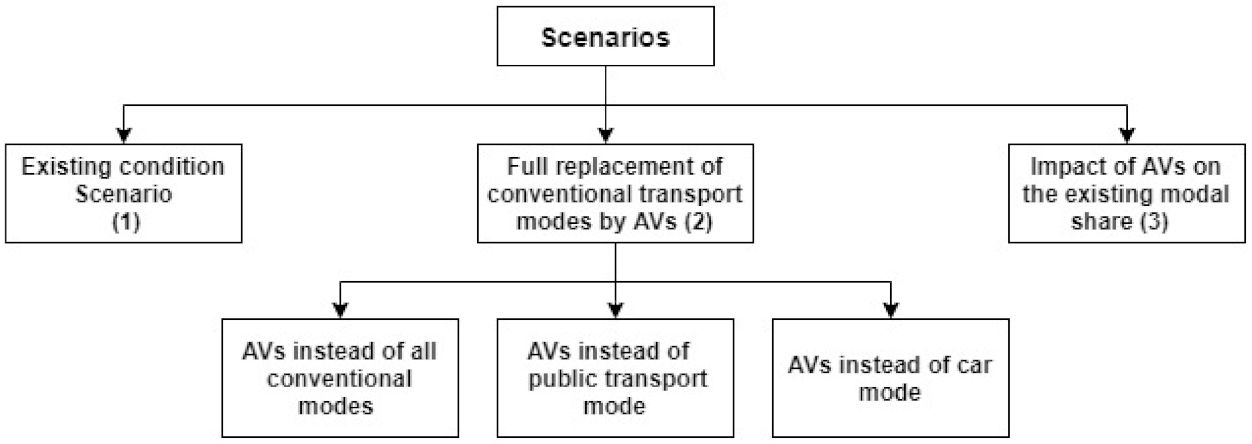
The impact of AVs on different transport user groups is examined as well as the modal share through three scenarios: (1) a simulation and optimization of the existing condition through a representative household sample size; (2) a simulation of the daily activity plans when all conventional transport modes, car users, and public transport riders are replaced by AVs; and (3) a simulation of daily activity plans when AVs are integrated into the daily activity plans concerning different VOTs of AVs (based on the VOT of conventional cars). The first scenario is studied to understand the existing behavior of travelers in which travelers are simulated and optimized based on their travel characteristics mentioned in the recorded daily activity plans (e.g., departure time, arrival time, transport mode, and activity location). The second scenario is conducted to estimate the impact of replacing specific groups of transport modes users by AVs, and finding the number of a replaced conventional cars by one AV; this scenario also represents simulating AVs with different travel demands. Finally, the third scenario is used for finding the impact of AVs on the existing conventional modal share based on different VOT assumptions to predict the future demand on each transport mode, where the assumptions are used for the absence of empirical results. The output of this study might be beneficial to policymakers in developing new strategies for new mobility services in urban areas.

The work is presented in the following way: After the introduction, Section 2 provides a literature review, and Section 3 explains the methodology. The results are presented in Section 4, and Section 5 includes the discussion of the results. Finally, a conclusion is drawn in Section 6.

2. Literature Review

AV as a mobility innovation provides a demanding research area, where travel time, travel cost, waiting time, safety, and ridesharing are the main determinants of using AVs [31,32]. AVs are expected to make an impact on the travel behavior of travelers, and this impact is considered a variable based on the preferences of people [23]. People usually try to minimize their travel time and increase their productive time (activity time) to maximize their benefit (utility) [33]. Several studies demonstrated that AVs could reduce the negative utility of travel time by enabling people to conduct more activities onboard compared to conventional transport modes, thus affecting the feeling and satisfaction of travelers positively [10,14,16]. For example, the trip length is evaluated less negatively when the trip is conducted by AVs instead of conventional cars, with consideration to the travelers’ preferences and their schedules [34,35]. Moreover, it is important to determine the target group of users, for example, whether AVs are suitable for elderly people or not [36]. AV users might face problems regarding their desired departure times, meaning that modifications may need to be made to the departure schedule for many commuters, which enables policymakers to develop a pricing scheme to control the use of AVs [37]. It is worth mentioning that the usage of AVs is affected by social factors, technology, and safety [38].

The implications of the availability of AVs on the demand of other modes are noted in several previously published studies. In the study of Berlin by Bischoff et al. [26], the authors examined the replacement of conventional taxis by autonomous taxis; they showed that 1 autonomous vehicle might replace 10 conventional taxis if the rides are shared, and 6 if the rides are not shared. Furthermore, the study presented an increase in the travel time by 17% when a conventional car was replaced by an autonomous taxi, but this time was assumed to be compensated by the zero parking time of an autonomous taxi. The replacement of conventional cars in Berlin might be achieved by 100,000 autonomous taxis, which allows travelers to switch to AVs to avoid the walking distance and the waiting time of public transport [26]. Bischoff et al. [26] assumed that travelers might stay at home waiting for the AVs rather than waiting at the stop station, but of course, other factors also have to be considered (weather, cost, etc.). A study in Zurich by Boesch et al. [39] showed that travelers are willing to wait for AVs for around 10 or 15 min at peak hours, while in other periods for nearly 5 min, which is very close to the average value in the case of public transport. The study also demonstrated that when the fleet of AVs contained 1000 vehicles, the average waiting times are 7 min and 5 min for peak and off-peak hours, respectively. Boesch et al. [39] of the study explained that waiting time in case of AVs might be higher than for public transport because AVs might drive straight to travelers based on travelers’ calls, but in case of public transport, travelers need to wait at public transport stops for a certain time, which might be less than the waiting time for AVs. The researchers of this analysis concluded that the acceptable waiting time of 10 min minimized the required fleet size of AVs by 90% even without active fleet management [39]. Thus, the acceptable waiting time has a great effect on the fleet size of AVs and the efficiency of the AVs fleet to fulfill the demand. Bischoff et al. [40] used 10 min of waiting time in the simulation of AVs to make a comparison to public transport and to study the impact of autonomous demand responsive transport (DRT) systems on the travel behavior of people in Cottbus, Germany. The researchers of this study used 60 s as the stop time for public transport and inserted a limited number of AVs with a fixed capacity of eight passengers. The time spent to collect travelers along the assigned path from origin to destination meant that the first rider would need to wait longer than others; this consideration is reflected in travel time calculations to avoid having travelers wait longer than an acceptable time, as demonstrated in a study of replacing a bus line with a fixed schedule by shared autonomous taxi in Berlin [41]. Leich et al. [41] assumed that the pooled AV mileage price per individual in Berlin is equal to 0.56 USD. This is demonstrated on a cost-based analysis, where the estimated cost of using AVs is 0.64 USD per kilometer and 0.34 USD per kilometer for taxi AVs, with four-seat capacity cars used for calculations [42]. Moreover, a study prepared by Fagnant et al. [28] concluded that AVs are expected to replace 9.3 conventional vehicles, supposing that no other modes are available in a pre-defined urban area of Austin city. The researchers of this study divided the city into blocks, where each block was assigned a certain fleet size of AVs to transport the travelers on that block, to minimize the waiting time and the vehicle miles traveled (VMT). The priority of the assigned fleet size of AVs for a block is the travelers in that block [28]. In case the demand is fulfilled, the idle AVs are used to solve the supply shortage of the neighboring block, if any. The authors of the analysis assigned AVs to travelers within 5–10 minutes, which represents the acceptable waiting time of a traveler [28]. The produced reduction in waiting time is 82% because of the applied method in distributing the AVs (blocks) [28]. Vosooghi et al. [43] studied the performance of shared autonomous vehicles (SAVs) and found that the performance is strongly affected by the size of the fleet, and that the impact of SAVs of more than four seats is limited. The impact of user preferences on SAVs was assessed in Paris city in [44]; the findings show that neglecting the preferences of travelers in the simulation impacts the use of SAV and consequentially influences future scenarios, as demonstrated by Kamel et al. [44]. As a continuity of the study of Kamel et al. [44], preference variations were also studied and integrated into the developed mode in [45], in order to find the variations on the outputs based on the classical simulation. A study conducted in Budapest, Hungary, showed that one AV can replace eight conventional vehicles, where travelers were exposed to 7–10 min waiting time [46]. Ortega et al. [47] showed that one AV can replace 2.4 conventional vehicles and minimize the travel time of workers and shoppers who use park-and-ride facilities in Budapest. Additionally, the demand for AVs is more likely to increase because other non-motorized users are potential users of AVs, based on a study conducted in the United States by Harper et al. [48]. The penetration of the AVs and the modeling of a transport system that considers AVs in the transport mode choice step were discussed by Török et al. [49], who addressed the impact on the route and the capacity of roads. Zambrano-Martinez et al. [50] presented a routing server to collect traffic data for an AV era that was applied in Valencia, Spain, and the results revealed improvements in the speed and the traffic congestion. Alonso-Mora et al. [51] developed a method to improve the routing of SAVs based on historical data collected by SAVs; a probability distribution was developed based on the collected data to predict the future demand in New York city, and the results showed a reduction in travel time and waiting time.

It was found in several studies that the AVs are expected to increase the VMT and in turn make an impact on the modal share by attracting travelers from other transport modes, such as a car, public transport, and non-motorized modes [52]. Milakis et al. [8] showed that AVs are expected to induce additional demand to the road network because of the longer trips. The replacement of all motorized trips by SAVs in Lisbon was studied by Martinez et al. [53]. The results of their study showed an increase in the VMT from 44% to 89% and a sharp reduction in parking spaces [53]. Two studies were conducted to evaluate the impact of AVs on the travel behavior of travelers by Auld et al. [54,55], who showed an increase in the VMT in Chicago metropolitan region when AVs appear on the market; their study examined the different levels of road capacity, varied fleet penetration of AVs, and different levels of VOT. Another study on travel behavior was conducted by de Almeida Correia et al. [56] in Delft, Netherlands, where private AVs were used instead of private cars; the results showed an increase in VMT and more utilization for the AV by the household members. Kröger et al. [57] studied the impact of AVs on the travel behavior in the United States and Germany by applying the spatial travel demand model, where different levels of fleet sizes and VOT were used. The results showed an increase in VMT and a shift from conventional transport modes to the AVs. Other scholars used agent-based modeling to simulate and study the impact of AVs on travel behavior, and they demonstrated that AVs are likely to increase the VMT [58,59,60]. These researchers showed that one AV can replace more than one conventional car, and they concluded that the AVs are expected to have a crucial impact on the modal share. Moreover, it was shown in the study of Cyganski et al. [61] in the city of Brunswick, Germany that introducing an AV fleet in the transportation system changes the modal share slightly.

One of the tools that are used in studying the behavior of traveler behavior is the MATSim tool [62]. MATSim is an open-source, activity-based microsimulation software; it is used to model the daily behavior of travelers (i.e., demand) and has the power to simulate large-scale projects (i.e., country) in a competitive time [63]. The optimization and simulation of daily activity plans are carried out by using MATSim, which applies the concept of a co-evolutionary algorithm based on flexible functions. The MATSim process loop includes the following five steps: initial demand, mobility simulation, scoring, re-planning, and analysis. MATSim uses the Charypar–Nagel utility function as a base for scoring plans. This function combines activity and travel utility, and this utility function is used for the scoring step regarding travelers’ plans, which is followed by a logit selection probability for the re-planning step [62]. Indeed, re-planning in the MATSim loop is conducted based on the genetic algorithm (GA) to generate alternatives (plans) and to be scored in the utility function (fitness function) [64]. GA does not generate the optimum solution; instead, it generates a plausible solution, which saves time for discovering possible alternatives [62]. Simulation of the activity chain requires scoring parameters that are obtained from the Vickrey bottleneck model (marginal utility of traveling, arrival late and early) [65]. These parameters assign penalties for an activity plan based on the Vickrey penalties’ pattern of departure time model per unit hour (h) (i.e., −6/h, −12/h, and −18/h for β_wait, β_trav, and β_late.ar, respectively) [65]. Based on the analysis of the opportunities and the recommendations about the impacts of AVs on travelers, different tools can be applied. The most dominant tool is MATSim, which is used in this research. The analysis aims at presenting the changes in travelers’ mobility parameters once AV is introduced as a new mode of transport.

Table 1. Summary of selected relevant studies.

Reference	Description	Location of Study	Method/Tool
[23]	The adoption of SAVs across 7 European countries, with VOT calculated per country	7 European countries	Stated preference survey; mixed logit model
[24]	Modeling of AVs and the regular cars to capture preference heterogeneity across individuals, with differences between country acceptance of AVs demonstrated	6 European countries	Stated preference survey; mixed logit model
[26]	Replacement of conventional taxis by autonomous taxis, where shared AV and individual rides were used by authors; findings show a higher replacement of conventional cars in shared rides compared to unshared	Berlin, Germany	MATSim
[28]	Serving travel demand by SAV based on providing certain fleet size for every zone; findings show a reduction in the waiting time, an increment in VMT produced, and the fleet size of SAVs determined	Austin, USA	MATSim
[34]	Impact of AVs on the travel time use; findings show AVs opening opportunities for other activities as well as extending some activities’ time	-	Mathematical model
[36]	Willingness of certain groups to use AVs; findings show different results per age group.	United States	American time use survey
[39]	Traveling by AVs considering different demands, with the impact of waiting time and the fleet size of AVs demonstrated	Zurich, Switzerland	MATSim
[40]	Impact of AV on the DRT; findings show that the public transport can be replaced by 300–500 autonomous DRT	Cottbus, Germany	MATSim
[41]	Replacement of bus lines with fixed schedule by SAVs; the fleet size that fulfill the demand on the bus line was determined	Berlin, Germany	MATSim
[47]	Simulation of the daily activity plans of travelers when park-and-ride system is integrated with the AVs; findings show reduction in travel time and increase in VMT	Budapest, Hungary	MATSim
[48]	The performance of SAVs when fleet size is changed, and the impact of changing the capacity of SAV on the mobility of people.	Rouen Normandie metropolitan area, France	MATSim
[54].	The importance of user preferences on the modal share is demonstrated. Neglecting the preferences of people in molding affects the quality of the outputs.	Paris, France	MATSim
[55]	The impact of AVs on the travel demand considering VOT, fleet size. The decrease in the VOT leads to increase in the VMT.	Chicago, Illinois, Metropolitan Area, USA	POLARIS
[58]	A comparative study between two countries regarding the travel behavior of people towards AVs. Germany will have lower increase in VMT and higher use of AVs.	Germany and the United States	Aspatial travel demand model (mathematical model)

presents the summary of the relevant studies, where the description, case study location, and the used methods are presented per study. It is worth mentioning that a discussion of the content of the table was presented earlier in this section. The first two studies focus on the acceptance of AVs and SAVs. It is also noted that different studies focus on the impact of AVs on the travel time and the VMT, and the determination of fleet size based on different travel demands. The previous studies show different outputs with similar trends (i.e., increased VMT, replacing more than one regular car by one AV, and decreased travel time), while few studies focused on the impact of AVs on the modal share by taking into consideration the different values of the VOT. In this study, we provide more detail about the mobility parameters generated from the simulation, such as utilization, drop off time, pick up time, and so on. This study forms one of the first studies that assesses the impact of AVs on the mobility of different groups of people (car users, and public transport users) and on the modal share by considering specific penetration levels of AVs and different VOTs for the travelers. It is noted that MATSim is a common tool used for implementing studies with different purposes due to its flexibility, and it provides an open development platform as an open-source software.

3. Methodology

3.1. Case Study

The integration of AVs in the daily activity plans of 8500 travelers, who recorded their daily activity plans in Budapest, is visualized as shown in Figure 1. The sample contains data comprising 8500 actual activities from households in Budapest (i.e., daily activities of 8500 travelers from different houses in Budapest); this is considered as a representative sample for the population of Budapest as well as the modal share of the city [66]. The data were collected and aggregated in 2014 by the Hungarian Census Bureau, which conducts a periodic survey every 10 years [67]. The sample contains information about the daily travel behavior of inhabitants such as activity type, transport mode, departure time, arrival time, parking search time, parking fees, and other sociodemographic variables. The proportions of different activity types are 51.5% work, 16.4% education, 15.4% shop, 13.5% other, and 3.2% leisure.

The sample was scaled to the population of Budapest city to consider the traffic conditions [62]. Budapest’s population was estimated based on the publicly available data of the National Hungarian Census Bureau; according to the bureau, the city of Budapest has around 1.7 million inhabitants, which is about the 18% of the Hungarian population [67]. Figure 1 and Figure 2 depict the road network, the 23 districts of Budapest, and the origin and first destinations of each traveler. The length of the road network in Budapest is around 8000 km including all classes of roads (around 650 roads with length greater than 1 km with a mean length of 3 km) based on the OSM within the boundaries of the city [68].

3.2. Conceptual Assumption

The changes in the travel behavior, starting from the time when AVs were integrated into the existing daily activity plans of travelers, were examined here. Three scenarios were simulated using MATSim, as shown in Figure 3. In the first scenario, two steps are conducted. The first step is the simulation of the existing condition (calibrating the model), which includes studying the existing condition without changing anything in the characteristics of the collected daily activity plans of the travelers. This step aims at simulating the real behavior of people based on the exact records, where the parameters of the model are estimated. The second step involves simulating and optimizing the daily activity plans by introducing changes in the plans, such as travel departures. The base scenario, which is used later, is the optimized one (in the second step).

The second scenario is made up of three sub-scenarios that include different groups of users. In the first sub-scenario, the conventional transport modes are replaced with AVs; this sub-scenario involves finding the required fleet size (i.e., number of vehicles) of AVs and calculating some mobility components, such as VMT. In the second sub-scenario, there is the substitution of public transport modes by AVs, while the third sub-scenario concerns car users, in which cars are replaced by AVs. In the second scenario, components such as waiting time and VMT were discussed.

The third scenario intends to find the impact of AVs on the current modal share when AVs appear on the market, specifically by considering the different VOTs of AVs. The costs of time spent (i.e., the marginal utilities of travel time) in AVs are compared to those of the conventional cars in the range of 90% to 50% with a 10% reduction, for example, 80% of VOT in the case of a conventional car. A fixed fleet size of AVs is set to see the impact of VOT on the usage of the fixed fleet. In order to achieve this goal, the data are prepared for the simulation by using MATSim.

3.3. Tool Description

Data preparation for the simulation was carried out, where all data files were converted to XML files (the daily activity plans, road network, and public transport network). The road network’s components of Budapest were extracted from OpenStreetMap (OSM) with the support of the JOSP MATSim plugin [69], while public transport data were taken from BKK [70], in the form of the General Transit Feed Specification (GTFS) files. A specific contribution in MATSim (Java code) was used to convert GTFS to a transit schedule file (XML) based on a pre-developed code in Java programming language [71]. All geographic data should be consistent in the form of text and coordinate systems, such as road networks, public transport networks, and activities’ locations. The coordinates were transformed to one reference coordinate system (EPSG: 3857) using the Eye4Software Coordinate Calculator software [72]. This software can convert one coordinate system to another with flexible and competent time using different projection types.

Table 2. Collected data and information.

Item	Description
Plans/diaries	Activity type, activity location, multimodal travel chain, activity duration, and scheduling
Road network	Link and nodes (coordinates), flow directions, the number of lanes, speed, capacity, length, allowed modes in each link, and toll road strategy
Public transport	Routes, locations, and name/number of stop stations, schedule, vehicle types and number/ID, capacity, speed, fleet size, working hours, and fare
Facilities	Locations (coordinates), type, and active time (opening hours)

shows a summary of the contents of some input files based on MATSim modules [62,73]. The plans/diaries consisted of 8500 activity plans; the road network XML file contained components of roads (e.g., speed), public transport network (e.g., schedule), and facilities that form the point of interest.

The second step, after the preparation of the data, was the simulation of the data. The process of the simulation and optimization in MATSim went through a loop called the “MATSim process loop”. This loop was executed (mobility simulation, scoring, and re-planning) by several iterations to guarantee the maximum scoring value (Figure 4). Each box in the figure is explained later.

3.4. Scheme of the Analysis with a Description

Initially, the 8500 daily activity plans were set as the demand, and they were loaded on the road network by using an integrated mobility simulator (named MobSim) in MATSim (see Horni et al. [62]). It is worth mentioning that MATSim 0.10.1 was used in this study. MobSim represents dynamic traffic modeling, which uses queue-based simulation (travel speed, flow capacity of a link, and car-following model). It is worth mentioning that the MATSim default transport mode is the car, while other modes (walking, biking, and using public transport) are recognized based on their operational characteristics. This recognition was performed in a teleportation module. The teleportation process was based on parameters in the configuration file, which enables the Qsim (i.e., MATSim’s default mobility simulator that is used to define the schedule of parameters in executing the plans) to simulate all modes other than the car, based on travel time, distance, and speed factors [62]. Qsim is the engine that loads the plans into the road network, based on a first-in-first-out (FIFO) strategy and identifies the capacity factors to represent the population. Here, Qsim was used as a mobility simulator to define which plan is to be implemented after both the re-planning process and the scoring steps are performed. A routing algorithm called Dijkstra’s algorithm was used to assign the best route to each individual; the chosen best route was then scored in the scoring step based on the chosen transport mode (i.e., tariff) [33].

In the scoring step, a utility function that combines both activity and travel parameters was applied. This utility function used a positive score for performing activities and a negative score for traveling. The total utility of a plan can be determined by the Charypar–Nagel function, as shown in Equation (1) [64]. The first part is the disutility (marginal utility) of traveling by using a chosen mode. This first part depends on the travel time, travel distance, and travel cost. On the other hand, the second part is the utility of performing an activity, which depends on the Vickrey model [62]. Here, travelers would try to maximize their benefits from executing the daily plan by deciding which one plan to select from several proposed options (see re-planning step). For example, travelers can minimize the time and cost of the travel, maximize the number of activities per day by saving time or by choosing different routes, different departure times, and different activity locations. The maximum benefit that can be obtained from conducting activities, the minimization of lost time in traveling, and the incurred cost in using modes of transport are addressed in Equation (1), which is the summation of the obtained benefits from travel time and performing activity:

$$V_{\mathrm{plan}}={\displaystyle \sum }_{\mathrm{i}=0}^{\mathrm{n}}(V_{\mathrm{act},\mathrm{i}}+V_{\mathrm{trav},\mathrm{i}}).$$

(1)

The first part is the activity side (V_act,i), while the second part is the traveling disutility side (V_trav,i). V_plan is the utility of performing a selected plan; V_act,i is the utility of performing the activity, which is always positive; and V_trav,i is the disutility derived from traveling to and from an activity. In more detail, Equation (2) presents the second part of Equation (1):

$$\begin{array}{c}{V}_{\left(\mathrm{trav},\left(\mathrm{mode},\mathrm{i}\right)\right)}=A_{\left(\mathrm{mode},\mathrm{i}\right)}+{\beta }_{\mathrm{trav},\left(\mathrm{mode},\mathrm{i}\right)}\ast {TT}_{\left(trav, i\right)}+{\mathsf{\beta }}_{\left(\mathrm{m}\right)}{∆}_{\left(\mathrm{m},\mathrm{i}\right)}+\\ (B_{\left(\mathrm{d},\left(\mathrm{mode},\mathrm{i}\right)\right)}+{\beta }_{\mathrm{m}}\ast {\gamma }_{\left(d, mode,i\right) }){\mathrm{Dis}}_{\left(\mathrm{trav},\mathrm{i}\right)}+{\beta }_{\left(\mathrm{transfer}\right)}\ast Y_{\left(\mathrm{transfer},\mathrm{i}\right)}.\end{array}$$

(2)

where trav stands for travel, mode means a transport mode, i means an activity, and d means a distance. A_{(mode, i)} is a transport mode-specific constant; β_{trav,(mode, i)} means the marginal utility of traveling; TT_(trav,i) means the travel time from activity_(i) to activity_{(i + 1)}; β_(m) stands for the marginal utility of money; ∆_(m,i) stands for the rate of change in the monetary budget caused by fees; β_{(d,(m, i))} stands for the marginal utility of distance; γ_(d,mode,i) stands for the mode-specific monetary distance rate; Dis_(trav,i) is the traveled distance between activity_(i) and activity_{(i + 1)}; β_(transfer) stands for the public transport transfer penalty; and Y_(transfer,i) stands for the existence of a transfer between the previous and the current plan (where 1 is yes, and 0 is no).

The utility function of activity depends on the duration of the activity, the arrival of a traveler with respect to the opening time of an activity (late, leave early, waiting, short duration), where Vickrey’s bottleneck congestion model penalties are applied for the activity utility [62]. The following logarithmic form is used to calculate the positive utility, which is shown in Equation (3) [64]:

$$V_{act, i}\left(t_{act, i}\right)={\beta }_{act} .t_{\ast ,i }. Ln\left(\frac{t_{act, i}}{t_{0, i}}\right)$$

(3)

where β_act is the marginal utility of performing an activity at its typical duration (t_*), while t_act is the actual performed activity duration. The t₀ is a scale parameter related to the minimum activity duration and its priority (or its importance). These equations were applied to the 8500 daily activity plans based on the route, the cost of a travel per kilometer, and the cost of the individual condition with respect to the activity time (Vickrey’s model).

Some changes/innovations were made in each traveler’s daily plan to find the maximum scoring, such as the changing of the departure time, the changing of the transport mode, and the changing of the route, as described in the re-planning step, which is a genetic algorithm (GA) process [62]. In the re-planning step (Figure 4), which is a learning mechanism in MATSim, the agents/travelers can improve their plans in each iteration until the maximum score and steady-state conditions are reached. The evaluation of the selected plans is executed based on preset strategies, for example, the possibility of changing the leg mode, re-using the previous bad plan, or identifying the maximum plans per traveler and the percentage of the selected plans to go through innovations (i.e., re-route, change leg mode, time allocation). The multinomial logit (ML) model is used for plan selection after generating alternatives (in the re-planning step) [62]. The alternatives are generated by making changes to the daily activity plans, such as changing the departure time, transport mode, and route. The same model (i.e., ML) is applied for calculating the probability of the travelers using a specific mode based on the distribution of the utility function [74]. The loop is executed several times, starting with evaluating the current daily activity plans, then making several changes to the departure time, transport mode, route, and the location of activity each iteration, until the maximum score is obtained for the system.

In case of AVs, the MATSim loop was applied but with specific characteristics. The dynamic vehicle routing problem (DVRP) algorithm, which is incorporated in the MATSim, matches the travelers who have the same schedule in order to optimize the used fleet size of AV, for example, by identifying the first traveler to pick up [75]. The DVRP optimizer is updated with the occurred changes in the daily activity plans, the fleet of the AV, or the traffic situation. In case of changes, it informs the MATSim of the new route or schedule, and the plan can go through the MATSim loop again. The AVs’ initial locations on the road network are randomly distributed by the distribution algorithm incorporated in MATSim [62]. The applied AVs are 4-seated, fully automated vehicles, and the type of use was individual ride. The simulation of AVs in MATSim requires a selection of the random fleet size of AVs to simulate and optimize the daily activity of the travelers; this fleet size of AVs depends directly on the acceptable waiting time of the travelers and the locations of the travelers. The acceptable waiting time in this study was set around 10 min, which almost equals the spent time in parking a car or the waiting time at a public transport stop plus access and egress walking time [26]. Another parameter that needed to be set in MATSim is the travel cost, which, in this research, was set for each transport mode, while the AVs’ fare was set based on the literature. The AVs’ cost is less than a car’s and more than the expense of the public transport since there are no drivers’ wages, and the costs of the maintenance and the depreciation is distributed over all users [62]. Moreover, a traffic flow capacity factor of 1.5 was used to reflect the traffic congestion since the capacity of a road segment carrying an autonomous vehicle was claimed to be 1.5 times the conventional car’s because machine efficiency is higher than human efficiency [74]. Particularly, the perception–reaction time and the positioning accuracy of the driving of a machine is faster than a human’s, which was proven by a study of Tientrakool et al. [76]. It was estimated that the highway capacity might be increased by 43% with vehicle sensors and up to 300% with vehicle-to-vehicle communications, as stated by Childress et al. [77] and Olia et al. [78], respectively. In this study, a 1.5 multiplier to the capacity factor was applied after scaling the 8500 household travelers to the population [29]. The evaluation of the simulation’s output was based on the scoring curve, the travel time, the travel distance, and the waiting time in the case of AVs. The operating cost that was used in this study for AV is 0.34 USD per km [42]. Additionally, 90%, 80%, 70%, 60%, and 50% of the marginal utility of the travel time of conventional cars were applied for AVs, as shown in Scenario 3. Moreover, as demonstrated in the literature, the marginal utility of traveling in AV is less than that in a conventional car [79].

3.5. Model Development

The parameters of the base model that combines both activity and travel utility and that captures future changes were estimated to predict the variations in the demand and the travel behavior of the travelers when changes occur. Initially, the statistics of modal share (actual mode shares of the case study) and the travel distance included in the recorded data of the daily activity plans of the travelers were used as a reference in determining the parameters, such as the mode choice model, and the speed of other than car transport modes [43,63]. The outputs of the simulation should converge enough to the actual collected data statistics, such as the modal share, and the traveled distance [80]. It is worth mentioning that the Charypar–Nagel and Vickrey bottleneck models were applied in developing the model as described in Equation (1), and the “typical” Vickrey bottleneck congestion model was used, in which the parameters of the models considered the opportunity cost distribution of time, where the saved time from traveling can be assigned to the activity time [62], as the following:

• marginal utility of money: (βm) = +1 utility/monetary unit,
• marginal utility of performing: (βdur) = +6 utility per hour (u/h),
• marginal utility of traveling: βtravel = −6 u/h,
• marginal utility of waiting: βwait = 0 u/h,
• marginal utility of short activity: βshort = 0 u/h,
• marginal utility of being late: βlate = −18 u/h,
• marginal utility of leaving early: βearly = 0 u/h.

Table 3. Traveling disutility parameters.

No.	Parameter	Comments
1	BrainExpBeta (scale μ)	Plan selection or choice; multinomial logit model selection between plans; value of 2 is applied (the default is 1, and 2 is recommended)
2	Marginal utility of money	Value should be positive because it has a positive impact on utility
3	Marginal utility traveling time	Using a car in traveling may involve paying more money but maybe decrease travel time
4	Marginal utility traveling distance by mode	No mode choice logit model, assumed to be zero; time rate and unit price are applied
5	Monetary distance rate	Car has a greater negative value than other modes (conversion of distance to money; see Table 4)

explains the applied utility parameters in simulating the daily activity of the travelers based on the utility function in MATSim. The logit model scale factor (μ) is used to scale the scoring. The μ is multiplied by the typical Vickrey model, such as early/late arrival to the activity. The monetary factors (marginal utility of money), the traveling factors (marginal utility of money based on distance or time), and the fee rates of each transport mode (monetary distance rate) are used as parameters to maximize the utility of the travelers in conducting their activities.

Table 4. Modes and marginal utility parameters.

Parameter	Calibrated Values
Marginal utility of performing activity, βduration	+6
Marginal utility of money, βc	+0.0018
Monetary distance rate (per meter)	−0.39 car, −0.0375 PT, −0.005 bike, −0 walking
Marginal utility of traveling for all modes(time), (βt)−	−2.5 car, −0.5 PT, −0.3 bikes, −0.1 walking
Constant, βo	−0.2 car, 3.92 PT, −17.81 bike, 2.64 walking

presents the parameters that were used in this study. The change in monetary distance reflects the toll or fare incurred when traveling from one geographical location to another. The monetary change rate value for each mode was calculated based on several parameters, for example, the engine type of the vehicle, the insurance, and the depreciation. Around 39 Hungarian Forint (HUF)/km and 5 HUF/km are used for cars and bicycles, respectively, as derived from the records (i.e., daily activity plan records) and from the tariff in Budapest [46,81]. Similarly, in case of public transport, the monetary change was calculated based on the ticket type and the distance traveled, it was estimated to be around 37.5 HUF/km. The monetary change per distance is negative because a traveler must pay money for a travel.

When developing the calibrated model, the values were obtained after many runs with MATSim. In each run, a different value of transport mode constant and marginal utility of traveling of each transport mode was used to calibrate the model. The outputs of the simulation in each run were checked (the modal share in the last iteration should coincide with the modal share of the first iteration) by considering the average travel distance of the simulation and the first iteration [62]. The final values were used in the base scenario, where the optimization of the existing condition model was conducted. In more detail, as presented in Table 4, public transport has a marginal utility of travel time less than a car and an AV. Moreover, the default value of the marginal utility of travel time is −6 for all modes [62]. The default value for performing an activity is +6 based on the Vickrey bottleneck model. The marginal utility of money is related to the traveler, and its default value is +1 (it is always positive), since having more money means few negative effects in terms of the travel cost. The marginal utility of money was calibrated and set to +0.0018 after many trials to reflect the impact of money on the behavior of the travelers and to consider the local currency of the case study.

As a result of the calibration process, the transport model of the city of Budapest was developed. In particular, the model was found to be very helpful in forecasting the changes in demand when a policy is changed. The simulations were conducted after setting the parameters in the tables; all travelers were processed through the MATSim loop.

When building the existing model, several runs with different iterations ranging from 5 to 200 were conducted to fix errors, to calibrate the model, and to study the changes in the scoring curve. The travelers’ activities were evaluated based on the Charypar–Nagel function and the Vickrey model. Thus, the duration of the activity, the arrival time, and the departure time of the travelers were scored, while the selected transport mode and the best route were evaluated/scored by applying the Charypar–Nagel function (see Equation (2)) based on the travel time and travel cost. Innovations (i.e., changes in the daily activity plans of the travelers) were made in the re-planning process in the daily activity plans of the travelers, and each time they were processed through the MATSim loop (MobSim, then scoring) for optimization. In the case of AVs, the best route, the minimum travel time, the minimum cost, and the minimum waiting time were updated. A steady-state condition was required in order to reach the maximum derived utility by conducting an activity plan, where no significant benefit can be obtained from changing the travelers’ plans (scoring value becomes fixed).

4. Results

The results and outputs of the simulations are discussed in the following subsections. Scenario 1 describes the base model for Budapest, and it is also used for comparisons. Scenario 2 is used for testing the hypothesis that the AV can decrease the number of conventional transport modes on the road network. Scenario 3 tests the hypothesis that the AV affects the existing model share to some extent where people continue using conventional modes in the AV era. The simulation runs are stopped when the maximum utility of activity plans and the steady-state point are reached.

4.1. Scenario 1: Modeling of the Existing Condition

This scenario aims to study the mobility of existing conditions using the daily activity plans of the travelers. The scenario consists of two parts. The first one is the result of the calibrated model, which was calibrated at the initial run; the second part consists of the simulation of the existing condition and the optimization of the travel time based on the changes in the travel departures. These two parts are conducted based on the parameters discussed in the previous section (Table 4). The result of the simulation of the 8500 daily activity plans is the modal share and the trip average distance at the initial run, which corresponds approximately to the recorded information in the daily activity plans of the travelers (i.e., statistics), as determined in the first step. The modal share is 2.3% bicycle, 26.8% car, 37.4% public transport, and 33.5% walking modes, while the average trip distance of a traveler per day is 3.87 km. The generated average trip time is 43.73 min. On the other hand, the second step of the scenario includes optimizing the travel time, and the result is 33.4 min, after the 30th iteration.

In part two, the travelers repeatedly change their transport modes, the time of departure, and the routes in each iteration to maximize their profits (utility value) [33]. The actual daily activity plans of the travelers are simulated regardless of any innovation on the components of the plans, as shown in Figure 5, while the steady-state condition in which the daily activity plans are optimized, as shown in Figure 6. It can be derived that the peak period, when the travel is realized, is from 7:00 to 9:00 and from 17:00 to 19:00. Technically, the simulation is enforced to stop when no significant change is noticed on the score of the system, which means that the travelers reach their maximum utility of the generated daily activity plans (i.e., at 30th iteration). This means that at the 30th iteration, no obtained benefit can be realized by changing the innovations strategies, such as the transport mode, the route, and the time of departure. In conclusion, the average daily travel time for a traveler is around 1 h and 28 min (multiplying the average number of trips by the average trip time), and it is reduced by 23% based on the results of the MATSim simulation, concerning mainly the innovation on the departure time. This scenario was considered as a basis for comparison with other scenarios. The final runtime of this scenario after setting all parameters is around 45 min using Intel® Core™ I7-7500U CPU, 2.70–2.9 GHz, and 8 GB RAM laptop.

4.2. Scenario 2: The Replacement of Conventional Transport Modes by AVs

The objective of this scenario is to find out the number of AVs that might serve different demands if travelers switched entirely to AVs. In this scenario, three simulations that represent different groups of travelers were executed. The first simulation (the first sub-scenario) is a full replacement of the conventional transport modes (walk, bike, car, and public transport) by AVs in the daily activity plans of 8500 travelers. The second simulation (the second sub-scenario) is a full replacement of conventional personal cars by AVs in the daily activity plans of 2356 travelers, and the third simulation (the third sub-scenario) replaces the public transport riders by AVs (3550 travelers). Scenario 2 is optimistic and simulates the ability of AVs to fulfill the demand of various forms.

It is worth mentioning that the result of the MATSim simulation of the existing condition produces trip durations of 33.4, 34, and 43 min for Simulations 1, 2, and 3, respectively. The simulation runs are stopped when the scoring reaches the steady-state and the maximum value (no benefit from changing in the travelers’ daily activity plans). The travel time does not regard the parking time, which was set around 9 min on average based on the collected data (including searching and parking operation). This value reflects the car users, who need to park their cars. As all conventional transport modes are replaced, based on the recorded parking time for those who used cars, the average parking time was found to be 6.8 min. Finally, 6.8 min were added to the first simulation and 9 min to the second simulation. With the presence of AVs, the simulations were repeated several times with different fleet sizes of AVs to find the suitable fleet size that serves the assigned demand and meets the criterion of acceptable waiting time (10 min). For instance, in the first simulation, 900, 1500, 2300, 2500, and 3000 AVs were tested, and we found that 3000 provided the best outcomes. As a result, fleet sizes of 3000, 300, and 425 AVs were selected for Simulations 1, 2, and 3, respectively. The mobility components, which account for AVs being used, are summarized in

Table 5. Travelers’ trip time components when AVs are used.

Simulation	Fleet Size	Average Trip Time	95th Percentile of Waiting Time	Average Waiting Time	Empty Driven Time	Pick-Up Time	Occupied Time	Drop-Off Time
		Minute			Hour Per Day
Full replacement of conventional transport modes	3000	18.75	11.2	2.83	797	568	5854	284
Full replacement of conventional personal cars	300	11.30	9.81	4.2	317	152	863	76
Replacing the public transport riders by AVs	425	9.56	9.77	3.63	453.2	238.8	1078.5	119.4

for each scenario. The 95th percentiles of passenger waiting times are 11.2, 9.81, and 9.77 min, for Simulations 1, 2, and 3, respectively. The produced 95th percentile waiting times satisfy the desired acceptable time of 95% of the travelers (i.e., around 10 min). The drop-off and pick-up times depend on the number of travelers in each simulation, where durations of 120 s for picking up a traveler and 60 s for dropping off were used. In the first simulation, the fleet of AVs is occupied for 5854 h per day and is empty for 797 h per day.

Figure 7 and Figure 8 show the fleet utilization and additional VMT per simulation in Scenario 1, respectively. Thus, the fleet utilization (the ratio between the pick-up time, drop-off time, occupied time to the pick-up time, drop-off time, occupied time, empty time) is 89%, and the AVs travel an additional distance of 14% (empty to occupied driven time). Similarly, in the second and third simulations, the fleet utilization is 77% and 76%, while the additional VMT is 17%, and 42%, respectively.

The average trip time of a person per trip is 18.75, 11.30, and 9.56 min for Simulations 1, 2, and 3, respectively. The result of Simulation 2 demonstrates that 1 AV can replace 7.85 conventional vehicles based on a 300 AV fleet size since the original conventional vehicle size is 2356 cars (2356 divided by 300). The runtime of the three simulations last 31 h and 53 min, 12 h and 3 min, and 17 h and 14 min for Simulations 1, 2, and 3, respectively, using Intel^® Core™ I7-7500U CPU with 2.70–2.9 GHz and 8 GB RAM laptop.

The intensity of the demand and the geographical distribution of the origin and the destination of the travelers (number and location of orders) define the occupancy of the vehicles per time. Figure 9 illustrates the results of Simulation 1, where the behavior of 3000 AVs at the 200th iteration serving 8500 travelers are presented. The fleet size can be derived from the time profile, where the sum of the pick-up, the drop-off, the occupied, and the empty values at peak period (values in the y-axis means fleet size) is the fleet size. The ratio of occupied vehicles to the empty driven vehicles indicates the utilization of the fleet with respect to time at different period intervals. Figure 10 illustrates the result of Simulation 2 of 300 AVs at the 200th iteration serving 2356 travelers. Similarly, Figure 11 illustrates the result of Simulation 3 of 425 AVs at the 200th iteration serving 3550 travelers. The gray area means that the vehicle is on the way; the red line means departure, and the blue line means arrival. From the figures, the distribution of demand with time is comprehensible, such as the peak period. The white area represents the unused times of the vehicles during the day. It is worth mentioning that a reduction of the fleet size from 3000 AVs to 1400 AVs produces a large increase in the waiting time since the number of the travelers is larger than the number of AVs in the fleet. In Figure 10 and Figure 11, it is shown that the peak periods of Simulations 2 and 3 are different, as well as the movement patterns, which reflect the variations in the activity locations, the departure times, and the arrival times. The distribution of the second peak period (i.e., evening time) over time is flatter than the morning period, which reflects that people are more flexible when they return home. In essence, these figures are useful in following up the travel of people over time. The figures were developed after certain iterations, where the relocations of the fleet size, the travel time, and the waiting time are optimized.

4.3. Scenario 3: The Impact of Introducing AVs on the Existing Modal Share

The integration of AVs in the daily activity plans of the travelers was simulated in Scenario 3. The simulation includes different cases based on the marginal utility of a conventional car. Each case includes various values of marginal utility of traveling in AVs based on the marginal utility of traveling in a conventional car. The values were 90%, 80%, 70%, 60%, and 50% of the marginal utility of conventional cars. Thus, five simulations (cases) were conducted, and the results are recorded in

Table 6. Modal shares in relation to the different values of marginal utility of traveling in AVs.

Transport Mode	Existing Situation	Cases
		90% of VOT of Car	80% of VOT of Car	70% of VOT of Car	60% of VOT of Car	50% of VOT of Car
AV	-	20.6	22.2	23.7	25.4	28.4
Car	26.8	9.5	8.6	8.1	7.5	6.4
Public transport	37.4	28.8	27.3	26.1	25.2	23.5
Bike	2.3	2.9	2.8	2.9	2.8	2.8
Walking	33.5	38.2	39.1	39.1	39.1	38.9

. The modal share of the existing condition shows that the highest modal share is public transport (37.4%) and the lowest is the bike (2.3%). Introducing AVs brings changes in the modal share, as shown in Table 6. It can be easily concluded from the results that a slight change in AV marginal utility of travel time does not trigger major changes in the modal share. For example, when the marginal utility of traveling in AVs is 90% of the marginal utility of the travel time of a conventional car, the AVs’ modal share is 20.6%, while it is 22.2% when the marginal utility of traveling is 80%. On the other hand, the change from 90% to 60% generates an increase in the usage of AVs from 20.6% to 25.4%. The result of the simulation with 50% of cars shows a higher shift from public transport to AVs since the marginal utility of traveling in this simulation is closer to the marginal utility of traveling in public transport. Thus, the marginal utility of traveling in AVs affects the modal share differently, and it is not linear, as demonstrated in the five simulations. Additionally, the walking modal share increases when 90% of the VOT simulation is produced, where the simulation setting defines 0.75 km as an acceptable walking distance (selected acceptable distance), and some of the travelers originally use their personal cars even for a shorter than 0.75 km distance; this enforces people to choose walking as transport mode rather than personal cars. It is illustrated that the walking share remains around 39% (small variations are produced because the algorithm in the re-planning step process does not change the same plan in each run).

The modal shares of the simulations are depicted in Figure 12, which includes the existing condition and the five cases. The existing situation represents the current condition of daily activity plans of 8500 travelers using the conventional transport modes, while the other simulations represent the result of modal share when AVs appear on the market in relation to the different levels of marginal utility of traveling.

The mobility components of the travelers who switched to AVs are summarized in

Table 7. The travelers’ trip time components when 20% fleet size is used.

Simulations	Average Waiting Time/Trip (Minutes)	Empty Driven Time	Pick-Up Time	Occupied Time	Drop-off Time	Fleet Utilization	Additional VMT	Fleet Average Served Request (#)
		Vehicle-Hours Per Day
90% of VOT	9.9	1541.72	310.10	2850.61	155.05	54.1%	68.3%	2.10
80% of VOT	9.8	1647.64	334.52	3065.93	167.27	53.7%	68.4%	2.25
70% of VOT	10.0	1831.89	365.53	3342.72	182.76	54.8%	68.0%	2.47
60% of VOT	10.5	2107.78	398.67	3807.39	199.33	55.4%	67.6%	2.76
50% of VOT	11.2	2481.40	440.88	4307.53	220.38	57.6%	66.7%	3.01

. The fleet size of AVs was set at 1700 to simulate the condition where people are familiar with technology and have enough trust in the technology to use AVs. The average waiting time is 9.9, 9.8, 10, 10.5, and 11.2 min for 90%, 80%, 70%, 60%, and 50% of VOT, respectively. It can be concluded that as the AV usage increases, the waiting time and the fleet average served request (i.e., the average number of the travelers per AV) increases as well. The fleet utilization is the ratio between the time when the fleet is occupied, picking up passengers, and dropping off passengers to the total time of driven time (occupied and empty), picking up, and dropping off the passengers, and this ratio ranges from 53.7% to 57.6%. As the fleet utilization increases, the efficiency of the fleet slightly increases as well, which means that more passengers are attracted by AVs. All simulations show additional VMT, which is generated from the empty driven time by the fleet. The highest is in 80% of VOT simulation, and the lowest is in 50% of VOT simulation. The increase in the VMT is mainly affected by the geographical location of the activities (i.e., distribution of the travelers on the network), and the fleet size of AVs. Therefore, the relation between the usage of AVs and the VMT is not straightforward, as demonstrated in the result of the five cases. The pick-up time and drop-off time are calculated based on the number of the travelers served by AVs. The pick-up time for a traveler is 120 s, and the drop-off time is 60 s, as derived from the literature [82].

5. Discussion

The transport demand is defined as a derived demand, where people use transport modes to access activities rather than obtaining direct benefits from traveling. The travel time cannot be eliminated, but it can be minimized or converted to productive time by conducting onboard activities and using the faster and more comfortable transport mode. The travel time minimization is reflected in the willingness of people to pay for a travel reduction, which is based on the VOT. The VOT is not equal for all transport modes, and it is different for one person or another. People give value to their travels according to different factors, for example, the willingness of high-income people to pay money to reduce the travel time is higher than that of low-income people. The recent advancement of AVs, which have different characteristics from conventional transport modes, has an impact on the VOT of people. The switch to AVs may decrease the VOT and potentially the negative impacts of travel time. Thus, this paper examines the impact of variations of VOT on the usage of AVs and the consequences on the modal share, as well as the travel behavior of people.

The three scenarios depict the existing condition and evaluate the impacts of AVs on travel behavior, such as the changes in the modal share and VMT. In Scenario 1, the travel behavior of the existing condition of the travelers is estimated, such as the travel distance and the travel time. In Scenario 2, the full replacement of conventional transport modes by AVs is studied, where the average travel time is reduced. The car travelers’ group is replaced by AVs, and the simulation demonstrates that one AV can replace 7.85 conventional cars with an acceptable waiting time. The public transport mode is replaced by AVs, and it results in less travel time and more VMT.

Scenario 2 demonstrates that the travel time can be minimized based on the AVs fleet size, the utility of traveling in AVs, and the characteristics of the travel, such as the departure and arrival times. It is worth mentioning that the road capacity factors, fleet size, speed, acceptable waiting time, travel distance, distribution of AVs on the network, and the capacity of vehicles are the main features that are involved in evaluating the impacts of AVs on the traveler’s mobility. To be precise, the acceptable waiting time corresponds to the waiting time of the travelers at public transport stop/station, and the walking distance corresponds to the nearest stop/station since AVs provide a door-to-door service. However, in case of the car, it corresponds to the parking time. Thus, the actual time saved in Scenario 2 is more than the difference between the travel time by AVs and the travel time in the case of conventional transport modes. For example, 6.8 min should be added to the average trip time in conventional modes of Simulation 2, and 9 min in Simulation 1 (see

Table 8. Trip time comparison between the conventional modes and AVs.

No.	Scenario	AVs			Conventional Modes	Percentage in the Sample (%)	Time-Saving (min)
		AVs Fleet Size	95% Percentile Passenger Waiting Time	Average Trip Duration	Average Trip Time
1	Modeling of the existing condition (i.e., the second step)	-	-		00:33:24	100	-
2.1	Full replacement of conventional transport modes	3000	11.2	18.75	00:33:24	100	10.25
2.2	Full replacement of conventional personal cars	300	9.81	11.30	00:34:00	26.8	21.89
2.3	Replacing the public transport riders by AVs	425	9.77	9.56	00:43:00	37.4	34.46

). As a result, the applied AVs can transport travelers with acceptable waiting times and competitive travel times without additional demand for the network. Although this is out of the scope of this paper, based on the literature, it has to be mentioned that AVs can generate extra demand, such as demand from young people who do not have a driving license and may take more trips because of the ease of traveling [48]. Table 8 presents a summary of the obtained results from the MATSim simulations; it shows a comparison between conventional transport modes and AVs in Scenarios 1 and 2. About 95% of the travelers experience a maximum waiting time of around 10 min, as mentioned in the last column. This column summarizes the differences among the conventional transport modes and AVs in Scenarios 1 and 2. The time savings in Simulations 1, 2, and 3 are 10.25, 21.89, and 34.46 min, respectively, considering the added parking time to Simulations 1 and 2.

The purpose of Scenario 2 is to examine the power of AV technology on travel behavior. Practically speaking, the applicability of Scenario 2 may be seen as unrealistic or far from achievability, but it measures the potential decrease of the travel time and travel distance, and it simulates a fully automated environment.

Scenario 3 tests the impact of AVs on the existing modal share. The result of this scenario demonstrates that the cost of the time spent in AVs determines the usage of AVs. This scenario contains five simulations that are studied using a fixed fleet size of AVs. The results demonstrate that the usage of AVs depends on the cost of time spent traveling. As the cost of time spent in a transport mode decreases, the usage increases. The result shows that the AVs influence the use of cars and public transport. The car seems to be the most affected transport mode. Walking and biking, which are the two non-motorized modes, are affected slightly. For example, the biking modal share is not affected to a great extent because the cost of time spent in travel by using a bike is significantly less than that with AVs. Thus, shifting from bike mode to others is not substantial. The walking mode is exposed to larger usage in the simulation of 90% of the VOT, as the daily activity plans consist of travelers who use motorized modes to travel to their destinations in case the distance is less than or equal to 1000 m (i.e., walkable distance). It is worth mentioning that for other simulations (2, 3, 4, and 5), the walking modal share is almost constant, which comes up to the expectations. The maximum acceptable walkable distance, the travelers’ preferences, and the trip characteristics determine the shift to the walking mode. The results of the five simulations show an additional, accompanied VMT with the use of AVs, which is generated from the empty driven time. Moreover, the results show different fleet utilizations of the 1700 AVs that can be involved in determining the parking spaces for the idle AVs and also in defining the profits generated from the fleet of AVs. More usage of AVs and more intensity of the demand show a larger fleet utilization and less additional VMT.

The results demonstrate that the AVs might decrease the travel time and increase the VMT. The acceptability of people to AVs is likely to determine their usage. Practically speaking, some people might have technophobia, which means that accepting AVs as a transport mode for those people is not an easy task. The acceptability of people (not including those who have technophobia) to the AVs is determined based on several factors connected to the characteristics of AV and the preferences of travelers, such as shared or unshared riding and trip purpose. The level of the impact of AV on the existing modal share is affected by the VOT of people, which is not the same for all, and it is connected to different factors, such as income class, trip purpose, and other factors. The usage of AVs is affected by a change in the VOT, which represents the marginal utility of time over the marginal utility of cost of a particular transport mode and a specific trip. Moreover, the fleet size of AVs influences the usage of AVs as it becomes larger once the usage is higher.

The result of Scenario 2 affects policymakers as demonstrated in the impact of a full replacement of conventional transport modes by AVs. It was shown that a smaller number of vehicles can cause the network to be loaded, while on the other hand, more VMT might be generated. This has an impact on the infrastructure of the depreciation of AVs because the fleet of vehicles drives more than required (empty driven). The empty driven time and additional VMT increase the cost of operation and consequentially decrease the profits due to the cost of maintenance and fuel (in the case of internal combustion engines). Using electric vehicles can reduce the cost of fuel and solve the problem of extra cost accompanied by empty driven vehicles. This requires infrastructure that fulfills the needs of these electric vehicles; an example of such requirements is charging stations.

On the other hand, Scenario 3 is considered more practical because it simulates all transport modes and studies the changes in the modal share with the presence of AVs. It provides valuable information to the policymakers regarding the usage of AVs concerning the VOT, which is affected by the sociodemographic of travelers and their preferences [8]. The predicted usage of AVs is determined when the VOT of travelers in AVs is known. City planners can obtain input data to their transport models when considering the reduction of cars, which affects the parking spaces and changes the land use. For instance, the high accessibility of AVs determines the residential location of people, and fewer parking spaces affect the prices of real estate.

The findings of this study are consistent with the previous studies, for example, the AVs increases the VMT and decreases the trip time. The magnitudes of VMT and the reduction in trip time are different than previous studies due to different physical factors, such as the locations of activities, road network, and public transport network. The findings of this study reveal new results compared to previous studies, such as the change in modal share, when VOT changes less than 50% of the VOT of a conventional car. The study finds negligible changes in the modal share when VOT is less than 50% of the VOT of conventional cars since the main modal share is AV in the motorized modes. Moreover, the used fleet size of AVs is 20% of the population, which does not simulate the initial stage of acceptability of AVs.

This study did not assess some factors that may also modify the usage of AVs and the impact of AVs on other transport components, in detail. For example, road network capacity, safety, and parking were not examined thoroughly in this research. Thus, these factors are recommended to be studied in further works. A wider sample may include different types of users, such as shoppers, workers, high-income people, or business trip cases. Additionally, different fleet sizes of AVs should be analyzed concerning various seats, and the possibility to share the ride is recommended to be studied.

One of the limitations of this study is that it did not focus on the impact of the AVs on the traffic conditions, and it concerned only travel time. Moreover, the impact of the full automation technology on the capacity of roads, and the interaction with the surrounding environments were out of the scope of this study. Furthermore, the parameters for the utility of travelers were defined by using the literature. The increase in the demand for using AVs from specific user groups was not considered, such as individuals with disabilities, who conduct only some activities due to their limited ability to move around on their own. Finally, the simulations in this study contained the sample size that includes representative households in Budapest city rather a generated synthesis population, which is recommended to be studied in the future and to be compared with the result of this study.

6. Conclusions

In this paper, daily activity plans were simulated and optimized through scenarios by using MATSim software. The simulations included the analysis of the existing condition through a representative household sample size by simulating the daily activity plans when all conventional transport modes, car users, and public transport riders are replaced by AVs, and simulating the daily activity plans of households when AVs are integrated into the daily activity plans using different VOTs of AVs.

Using the scenarios, we studied the current mobility of travelers and the impact of AVs on travelers’ mobility and the conventional modes. With MATSim, we used a genetic algorithm to optimize the daily activity plans based on the Charypar–Nagel utility function and Vickrey’s bottleneck model. Budapest was taken as a case study, and the result of the simulation of the base scenario is that the average traveled distance by a person per day per leg is 3.87 km and the average travel time is 33.4 min. In Scenario 2, the fleet size of AVs serving different demands was determined, which demonstrated that one AV replaces more than one car; the acceptable waiting time determined the required fleet size to serve a demand, and a reduction in travel time was obtained when AV is used as a replacement mode. In Scenario 3, the impact of AVs on the modal share is high, as the marginal utility of traveling in AVs becomes significantly lower than that in conventional cars. However, the impact is small on the non-motorized transport modes. The size of the population determines the number of cars that might be replaced by one AV because the occupancy of AV is affected by the geographical distribution and the intensity of the demand. As a result, 1 AV can replace 7.85 conventional cars with acceptable waiting time. It was demonstrated that the availability of AVs is expected to decrease the number of conventional cars on the market. Thus, the hypotheses were verified, namely that (1) the introduction of AVs on the market is expected to change the modal share of existing transport modes, (2) AVs can replace more than one conventional car, (3) using AVs decreases the travel time, and (4) using AVs produces additional VMT.

This study covered the impact of AVs on modal share, VMT, and travel time, where the perception of people and their VOT onboard of an AV were studied. The results of this research can be used as a reference for policymakers as well as future operators of AVs.

It is recommended that the result of this study be updated using daily activity plans of more recent years, and that the impact of COVID-19 on the mobility of people be considered. In addition, using different penetration levels of AVs on the market would be an interesting idea for a future study. Moreover, it is recommended that empirical results be used for making a comparison with this study to consider, for example, the actual VOT of travelers when they use AV. Additionally, it would be worth investigating the inclusion of novel transport modes that are becoming available on the market, such as e-mobility modes (electric cars, e-scooters), bike sharing, and car sharing. Finally, the economic impact of implementing each scenario is a good topic to be studied in the future.

References

1. Schoettle, B.; Sivak, M. Motorists’ Preferences for Different Levels of Vehicle Automation; University of Michigan, Transportation Research Institute: Ann Arbor, MI, USA, 2015. [Google Scholar]
2. Litman, T. Autonomous Vehicle Implementation Predictions: Implications for Transport Planning; Victoria Transport Policy Institute: Victoria, BC, Canada, 2020. [Google Scholar]
3. Jing, P.; Hu, H.; Zhan, F.; Chen, Y.; Shi, Y. Agent-based simulation of autonomous vehicles: A systematic literature review. IEEE Access 2020, 8, 79089–79103. [Google Scholar] [CrossRef]
4. Wiseman, Y. Self-driving car-a computer will park for you. Int. J. Eng. Technol. Automob. Secur. 2017, 1, 9–16. [Google Scholar] [CrossRef] [Green Version]
5. Antov, D.; Banet, A.; Barbier, C.; Bellet, T.; Bimpeh, Y.; Boulanger, A.; Brandstätter, C.; Britschgi, V.; Brosnan, M.; Buttler, I. European Road Users’ Risk Perception and Mobility: The SARTRE 4 Survey; IFSTTAR: Paris, France, 2012. [Google Scholar]
6. Pettigrew, S.; Talati, Z.; Norman, R. The health benefits of autonomous vehicles: Public awareness and receptivity in Australia. Aust. N. Z. J. Public Health 2018, 42, 480–483. [Google Scholar] [CrossRef] [PubMed] [Green Version]
7. Loeb, B.; Kockelman, K.M.; Liu, J. Shared autonomous electric vehicle (SAEV) operations across the Austin, Texas network with charging infrastructure decisions. Transp. Res. Part C: Emerg. Technol. 2018, 89, 222–233. [Google Scholar] [CrossRef]
8. Milakis, D.; Van Arem, B.; Van Wee, B. Policy and society related implications of automated driving: A review of literature and directions for future research. J. Intell. Transp. Syst. Technol. Plan. Oper. 2017, 21, 324–348. [Google Scholar] [CrossRef]
9. Coppola, P.; Esztergár-Kiss, D. Autonomous Vehicles and Future Mobility; Elsevier: Amsterdam, The Netherlands, 2019. [Google Scholar]
10. Janssen, C.P.; Kenemans, J.L. Multitasking in autonomous vehicles: Ready to go? In Proceedings of the 3rd Workshop on User Experience of Autonomous Vehicles at AutoUI’15, Nottingham, UK, 1 September 2015.
11. Hamadneh, J.; Esztergár-Kiss, D. Modeling travel behavior onboard of privately autonomous vehicle and shared autonomous. Veh. Ind. 2021, 8, 57–61. [Google Scholar]
12. Yang, J.; Coughlin, J.F. In-vehicle technology for self-driving cars: Advantages and challenges for aging drivers. Int. J. Automot. Technol. 2014, 15, 333–340. [Google Scholar] [CrossRef]
13. Pettigrew, S.; Cronin, S.L. Stakeholder views on the social issues relating to the introduction of autonomous vehicles. Transp. Policy 2019, 81, 64–67. [Google Scholar] [CrossRef]
14. Zhong, H.; Li, W.; Burris, M.W.; Talebpour, A.; Sinha, K.C. Will autonomous vehicles change auto commuters’ value of travel time? Transp. Res. Part D Transp. Environ. 2020, 83, 102303. [Google Scholar] [CrossRef]
15. Berliner, R.M.; Malokin, A.; Circella, G.; Mokhtarian, P.L. Travel-Based Multitasking: Modeling the Propensity to Conduct Activities While Commuting, 15-5018. In Proceedings of the Transportation Research Board 94th Annual Meeting, Washington, DC, USA, 11–15 January 2015. [Google Scholar]
16. Ettema, D.; Verschuren, L. Multitasking and value of travel time savings. Transp. Res. Rec. J. Transp. Res. Board 2007, 2010, 19–25. [Google Scholar] [CrossRef]
17. Cascetta, E. Random utility theory. In Transportation Systems Analysis; Springer: Berlin/Heidelberg, Germany, 2009; pp. 89–167. [Google Scholar]
18. Hess, S.; Bierlaire, M.; Polak, J.W. Estimation of value of travel-time savings using mixed logit models. Transp. Res. Part A Policy Pract. 2005, 39, 221–236. [Google Scholar] [CrossRef] [Green Version]
19. Aloulou, F. The Application of Discrete Choice Models in Transport. Stat. Grow. Data Sets Grow. Demand Stat. 2018, 5, 85–104. [Google Scholar] [CrossRef] [Green Version]
20. Ben-Akiva, M.E.; Lerman, S.R.; Lerman, S.R. Discrete Choice Analysis: Theory and Application to Travel Demand; MIT Press: Cambridge, MA, USA, 1985; Volume 9. [Google Scholar]
21. Athira, I.; Muneera, C.; Krishnamurthy, K.; Anjaneyulu, M. Estimation of value of travel time for work trips. Transp. Res. Procedia 2016, 17, 116–123. [Google Scholar] [CrossRef]
22. Mackie, P.J.; Jara-Dıaz, S.; Fowkes, A. The value of travel time savings in evaluation. Transp. Res. Part E Logist. Transp. Rev. 2001, 37, 91–106. [Google Scholar] [CrossRef]
23. Polydoropoulou, A.; Tsouros, I.; Thomopoulos, N.; Pronello, C.; Elvarsson, A.; Sigþórsson, H.; Dadashzadeh, N.; Stojmenova, K.; Sodnik, J.; Neophytou, S.; et al. Who is willing to share their AV? Insights about gender differences among seven countries. Sustainability 2021, 13, 4769. [Google Scholar] [CrossRef]
24. Etzioni, S.; Hamadneh, J.; Elvarsson, A.B.; Esztergár-Kiss, D.; Djukanovic, M.; Neophytou, S.N.; Sodnik, J.; Polydoropoulou, A.; Tsouros, I.; Pronello, C. Modeling cross-national differences in automated vehicle acceptance. Sustainability 2020, 12, 9765. [Google Scholar] [CrossRef]
25. Steck, F.; Kolarova, V.; Bahamonde-Birke, F.; Trommer, S.; Lenz, B. How autonomous driving may affect the value of travel time savings for commuting. Transp. Res. Rec. J. Transp. Res. Board 2018, 2672, 10. [Google Scholar] [CrossRef] [Green Version]
26. Bischoff, J.; Maciejewski, M. Simulation of city-wide replacement of private cars with autonomous taxis in Berlin. Procedia Comput. Sci. 2016, 83, 237–244. [Google Scholar] [CrossRef] [Green Version]
27. Kwok, S.; Schulte, J.; Hallstedt, S. Approach for sustainability criteria and product life-cycle data simulation in concept selection. In Proceedings of the Design Society: DESIGN Conference, Cambridge, UK, 11 June 2020; pp. 1979–1988. [Google Scholar]
28. Fagnant, D.J.; Kockelman, K.M.; Bansal, P. Operations of shared autonomous vehicle fleet for Austin, Texas, market. Transp. Res. Rec. J. Transp. Res. Board 2015, 2536, 98–106. [Google Scholar] [CrossRef] [Green Version]
29. Maciejewski, M.; Nagel, K. Simulation and dynamic optimization of taxi services in MATSim. Transp. Sci. 2013, 10–13. [Google Scholar] [CrossRef]
30. Trommer, S.; Kolarova, V.; Fraedrich, E.; Kröger, L.; Kickhöfer, B.; Kuhnimhof, T.; Lenz, B.; Phleps, P. Autonomous driving-the impact of vehicle automation on mobility behaviour. Inst. Mobil. Res. 2016, 122, 146–161. [Google Scholar]
31. Zmud, J.; Sener, I.N.; Wagner, J. Self-driving vehicles: Determinants of adoption and conditions of usage. Transp. Res. Rec. 2016, 2565, 57–64. [Google Scholar] [CrossRef] [Green Version]
32. Jing, P.; Xu, G.; Chen, Y.; Shi, Y.; Zhan, F. The Determinants behind the Acceptance of Autonomous Vehicles: A Systematic Review. Sustainability 2020, 12, 1719. [Google Scholar] [CrossRef] [Green Version]
33. MATSim Community. Multi-Agent Transport Simulation. Available online: https://github.com/matsim-org/matsim-code-examples/wiki (accessed on 11 November 2018).
34. Pudāne, B.; Molin, E.J.; Arentze, T.A.; Maknoon, Y.; Chorus, C.G. A Time-use Model for the Automated Vehicle-era. Transp. Res. Part C Emerg. Technol. 2018, 93, 102–114. [Google Scholar] [CrossRef]
35. Hamadneh, J.; Esztergár-Kiss, D. Potential Travel Time Reduction with Autonomous Vehicles for Different Types of Travellers. Promet Traffic Transp. 2021, 33, 61–76. [Google Scholar] [CrossRef]
36. Das, S.; Sekar, A.; Chen, R.; Kim, H.C.; Wallington, T.J.; Williams, E. Impacts of Autonomous Vehicles on Consumers Time-Use Patterns. Challenges 2017, 8, 32. [Google Scholar] [CrossRef] [Green Version]
37. Kim, C.; Jin, Y.-G.; Park, J.; Kang, D. The influence of an autonomous driving car operation on commuters’ departure times. Procedia Comput. Sci. 2019, 151, 85–91. [Google Scholar] [CrossRef]
38. Koul, S.; Eydgahi, A. The Impact of Social Influence, Technophobia, and Perceived Safety on Autonomous Vehicle Technology Adoption. Period. Polytech. Transp. Eng. 2020, 48, 133–142. [Google Scholar] [CrossRef]
39. Boesch, P.M.; Ciari, F.; Axhausen, K.W. Autonomous vehicle fleet sizes required to serve different levels of demand. Transp. Res. Rec. J. Transp. Res. Board 2016, 2542, 111–119. [Google Scholar] [CrossRef] [Green Version]
40. Bischoff, J.; Führer, K.; Maciejewski, M. Impact assessment of autonomous DRT systems. Transp. Res. Procedia 2018, 41, 440–446. [Google Scholar] [CrossRef]
41. Leich, G.; Bischoff, J. Should autonomous shared taxis replace buses? A simulation study. Transp. Res. Procedia 2018, 41, 450–460. [Google Scholar] [CrossRef]
42. Bösch, P.M.; Becker, F.; Becker, H.; Axhausen, K.W. Cost-based analysis of autonomous mobility services. Transp. Policy 2018, 64, 76–91. [Google Scholar] [CrossRef]
43. Vosooghi, R.; Puchinger, J.; Jankovic, M.; Vouillon, A. Shared autonomous vehicle simulation and service design. Transp. Res. Part C Emerg. Technol. 2019, 107, 15–33. [Google Scholar] [CrossRef] [Green Version]
44. Kamel, J.; Vosooghi, R.; Puchinger, J.; Ksontini, F.; Sirin, G. Exploring the impact of user preferences on shared autonomous vehicle modal split: A multi-agent simulation approach. Transp. Res. Procedia 2019, 37, 115–122. [Google Scholar] [CrossRef]
45. Al Maghraoui, O.; Vosooghi, R.; Mourad, A.; Kamel, J.; Puchinger, J.; Vallet, F.; Yannou, B. Shared Autonomous Vehicle Services and User Taste Variations: Survey and Model Applications. Transp. Res. Procedia 2020, 47, 3–10. [Google Scholar] [CrossRef]
46. Hamadneh, J.; Esztergár-Kiss, D. Impacts of Shared Autonomous Vehicles on the Travelers’ Mobility. In Proceedings of the 2019 6th International Conference on Models and Technologies for Intelligent Transportation Systems (MT-ITS), Kraków, Poland, 5–7 June 2019; pp. 1–9. [Google Scholar]
47. Ortega, J.; Hamadneh, J.; Esztergár-Kiss, D.; Tóth, J. Simulation of the Daily Activity Plans of Travelers Using the Park-and-Ride System and Autonomous Vehicles: Work and Shopping Trip Purposes. Appl. Sci. 2020, 10, 2912. [Google Scholar] [CrossRef] [Green Version]
48. Harper, C.D.; Hendrickson, C.T.; Mangones, S.; Samaras, C. Estimating potential increases in travel with autonomous vehicles for the non-driving, elderly and people with travel-restrictive medical conditions. Transp. Res. Part C Emerg. Technol. 2016, 72, 1–9. [Google Scholar] [CrossRef]
49. Török, Á.; Szalay, Z.; Uti, G.; Verebélyi, B. Rerepresenting Autonomated Vehicles in a Macroscopic Transportation Model. Period. Polytech. Transp. Eng. 2020, 48, 269–275. [Google Scholar] [CrossRef] [Green Version]
50. Zambrano-Martinez, J.L.; Calafate, C.T.; Soler, D.; Lemus-Zúñiga, L.-G.; Cano, J.-C.; Manzoni, P.; Gayraud, T. A centralized route-management solution for autonomous vehicles in urban areas. Electronics 2019, 8, 722. [Google Scholar] [CrossRef] [Green Version]
51. Alonso-Mora, J.; Wallar, A.; Rus, D. Predictive routing for autonomous mobility-on-demand systems with ride-sharing. In Proceedings of the 2017 IEEE/RSJ International Conference on Intelligent Robots and Systems (IROS), Vancouver, BC, Canada, 24–28 September 2017; pp. 3583–3590. [Google Scholar]
52. Soteropoulos, A.; Berger, M.; Ciari, F. Impacts of automated vehicles on travel behaviour and land use: An international review of modelling studies. Transp. Rev. 2019, 39, 29–49. [Google Scholar] [CrossRef]
53. Martinez, L.; Crist, P. Urban Mobility System Upgrade–How shared self-driving cars could change city traffic. In Proceedings of the International Transport Forum, Paris, France, 27–29 May 2015. [Google Scholar]
54. Auld, J.; Sokolov, V.; Stephens, T.S. Analysis of the effects of connected–automated vehicle technologies on travel demand. Transp. Res. Rec. 2017, 2625, 1–8. [Google Scholar] [CrossRef]
55. Auld, J.; Verbas, O.; Javanmardi, M.; Rousseau, A. Impact of privately-owned level 4 CAV technologies on travel demand and energy. Procedia Comput. Sci. 2018, 130, 914–919. [Google Scholar] [CrossRef]
56. De Almeida, C.G.H.; van Arem, B. Solving the User Optimum Privately Owned Automated Vehicles Assignment Problem (UO-POAVAP): A model to explore the impacts of self-driving vehicles on urban mobility. Transp. Res. Part B Methodol. 2016, 87, 64–88. [Google Scholar] [CrossRef]
57. Kröger, L.; Kuhnimhof, T.; Trommer, S. Does context matter? A comparative study modelling autonomous vehicle impact on travel behaviour for Germany and the USA. Transp. Res. Part A Policy Pract. 2019, 122, 146–161. [Google Scholar] [CrossRef]
58. Llorca, C.; Moreno, A.; Moeckel, R. Effects of shared autonomous vehicles on the level of service in the greater Munich metropolitan area. In Proceedings of the International Conference on Intelligent Transport Systems in Theory and Practice, Munich, Germany, 4–5 July 2017; pp. 4–5. [Google Scholar]
59. Liu, J.; Kockelman, K.M.; Boesch, P.M.; Ciari, F. Tracking a system of shared autonomous vehicles across the Austin, Texas network using agent-based simulation. Transportation 2017, 44, 1261–1278. [Google Scholar] [CrossRef]
60. Zhang, W.; Guhathakurta, S.; Khalil, E.B. The impact of private autonomous vehicles on vehicle ownership and unoccupied VMT generation. Transp. Res. Part C Emerg. Technol. 2018, 90, 156–165. [Google Scholar] [CrossRef] [Green Version]
61. Cyganski, R.; Heinrichs, M.; von Schmidt, A.; Krajzewicz, D. Simulation of automated transport offers for the city of Brunswick. Procedia Comput. Sci. 2018, 130, 872–879. [Google Scholar] [CrossRef]
62. Horni, A.; Nagel, K.; Axhausen, K.W. The Multi-Agent Transport Simulation MATSim; Ubiquity Press: London, UK, 2016; p. 620. [Google Scholar]
63. Nicolai, T.W. Integrating an Urban Simulation Model with a Travel Model; Berlin Institute of Technology (TU Berlin): Berlin, Germany, 2013. [Google Scholar]
64. Charypar, D.; Nagel, K. Generating complete all-day activity plans with genetic algorithms. Transportation 2005, 32, 369–397. [Google Scholar] [CrossRef] [Green Version]
65. Arnott, R.; De Palma, A.; Lindsey, R. A structural model of peak-period congestion: A traffic bottleneck with elastic demand. Am. Econ. Rev. 1993, 83, 161–179. [Google Scholar]
66. EPOMM. Tems-the Epomm Modal Split Tool. Available online: http://tems.epomm.eu/result_city.phtml?city=341&list=1 (accessed on 6 June 2021).
67. HCSO. Population Census in 2011. Available online: http://www.ksh.hu/nepszamlalas/copyright_eng (accessed on 6 June 2021).
68. OpenStreetMap Contributors. Open Street Maps. Available online: https://www.openstreetmap.org/#map=9/47.3509/19.1409 (accessed on 6 June 2021).
69. JOSM. Java OpenStreetMap Editor. Available online: https://josm.openstreetmap.de/wiki/Download#Java (accessed on 6 June 2021).
70. BKK. TransitFeeds.com. Available online: https://transitfeeds.com/p/bkk/42 (accessed on 6 June 2021).
71. Poletti, F. Public Transit Mapping on Multi-Modal Networks in MATSim. In Swiss Federal Institute of Technology; ETH Zurich: Zürich, Switzerland, 2016. [Google Scholar]
72. Softland-SRL. Eye4Software Coordinate Calculator, Version 8.0.7.1211; Softland SRL: Cluj-Napoca, Romania, 2019. [Google Scholar]
73. Balmer, M.; Axhausen, K.W.; Nagel, K. Agent-based demand-modeling framework for large-scale microsimulations. Transp. Res. Rec. J. Transp. Res. Board 2006, 1985, 125–134. [Google Scholar] [CrossRef]
74. Simoni, M.D.; Kockelman, K.M.; Gurumurthy, K.M.; Bischoff, J. Congestion Pricing in a World of Self-driving vehicles: An Analysis of Different Strategies in Alternative Future Scenarios. Transp. Res. Part C Emerg. Technol. 2018, 98, 167–185. [Google Scholar] [CrossRef] [Green Version]
75. Maciejewski, M.; Nagel, K. Towards multi-agent simulation of the dynamic vehicle routing problem in matsim. In Proceedings of the International Conference on Parallel Processing and Applied Mathematics, Torun, Poland, 11–14 September 2011; pp. 551–560. [Google Scholar]
76. Tientrakool, P.; Ho, Y.-C.; Maxemchuk, N.F. Highway capacity benefits from using vehicle-to-vehicle communication and sensors for collision avoidance. In Proceedings of the 2011 IEEE Vehicular Technology Conference (VTC Fall), San Francisco, CA, USA, 5–8 September 2011; pp. 1–5. [Google Scholar]
77. Childress, S.; Nichols, B.; Charlton, B.; Coe, S. Using an activity-based model to explore the potential impacts of automated vehicles. Transp. Res. Rec. 2015, 2493, 99–106. [Google Scholar] [CrossRef]
78. Olia, A.; Razavi, S.; Abdulhai, B.; Abdelgawad, H. Traffic capacity implications of automated vehicles mixed with regular vehicles. J. Intell. Transp. Syst. Technol. Plan. Oper. 2018, 22, 244–262. [Google Scholar] [CrossRef]
79. Bozorg, S.L.; Ali, S.M. Potential Implication of Automated Vehicle Technologies on Travel Behavior and System Modeling; FIU Digital Common: Tallahassee, FL, USA, 2016. [Google Scholar]
80. Kickhöfer, B.; Hosse, D.; Turner, K.; Tirachini, A. Creating an Open MATSim Scenario from Open Data: The Case of Santiago de Chile; Technical Report, VSP Working Paper 16-02; TU Berlin: Berlin, Germany, 2016. [Google Scholar]
81. BetterTec GmbH. Taxi Fares Are Based on the Current Taxi Tariffs of Budapest. Available online: https://www.bettertaxi.com/taxi-fare-calculator/budapest/ (accessed on 6 June 2021).
82. Moreno, A.T.; Michalski, A.; Llorca, C.; Moeckel, R. Shared autonomous vehicles effect on vehicle-km traveled and average trip duration. J. Adv. Transp. 2018, 2018, 1–10. [Google Scholar] [CrossRef] [Green Version]
Figure 1. Travelers’ origins in Budapest.
Energies 14 04163 g001
Figure 2. Travelers’ destinations in Budapest.
Energies 14 04163 g002
Figure 3. Proposed travelers’ behavior simulation scenarios.
Energies 14 04163 g003
Figure 4. MATSim execution steps.
Energies 14 04163 g004
Figure 5. Leg histogram showing the number of travelers per time (h) at initial condition (t0).
Energies 14 04163 g005
Figure 6. Leg histogram showing the number of travelers per time (hr) after 30 iterations.
Energies 14 04163 g006
Figure 7. Fleet utilization per simulation in Scenario 1.
Energies 14 04163 g007
Figure 8. Additional VMT per simulation in Scenario 1.
Energies 14 04163 g008
Figure 9. The time profile of AVs fleet size of simulation 1.
Energies 14 04163 g009
Figure 10. The time profile of AVs fleet size of Simulation 2.
Energies 14 04163 g010
Figure 11. The time profile of AVs fleet size of Simulation 3.
Energies 14 04163 g011
Figure 12. Modal share with the presence of AVs.
Energies 14 04163 g012