Arc Fault Detection Algorithm Based on Variational Mode Decomposition and Improved Multi-Scale Fuzzy Entropy

Abstract

Arc fault diagnosis is necessary for the safety and efficiency of PV stations. This study proposed an arc fault diagnosis algorithm formed by combining variational mode decomposition (VMD), improved multi-scale fuzzy entropy (IMFE), and support vector machine (SVM). This method first uses VMD to decompose the current into intrinsic mode functions (IMFs) in the time-frequency domain, then calculates the IMFE according to the IMFs associated with the arc fault. Finally, it uses SVM to detect arc faults according to IMFEs. Arc fault data gathered from a PV arc generation experiment platform are used to validate the proposed method. The results indicated the proposed method can classify arc fault data and normal data effectively.

1. Introduction

With the shortage of fossil fuels and increasing concern for the environment, demand for clean energies is increasing. Among clean energies, solar energy has been found to have the advantages of sustainability and cleanliness, attracting more and more attention. According to the reports of the International Energy Agency (IEA) and the International Renewable Energy Agency (IRENA) [1,2], the total installed capacity of the global photovoltaic industry has maintained a stable upward trend from 2011 to 2019.

At present, photovoltaic systems usually operate at a high voltage to save on the investment in cables [3,4,5,6,7,8]. For example, the DC voltage of a photovoltaic system in some places has reached 1000 V [9]. High voltage makes air more easily ionized and greatly increases the possibility of a photovoltaic DC arc [10]. In addition, a PV system is often placed in harsh conditions. Small creatures, high air humidity, and so on can also trigger photovoltaic DC arcs. If an arc is not detected in time, a continuous arc can generate high temperature plasma, which can severely damage the components of the photovoltaic system or even cause a fire. This kind of damage can severely affect the efficiency and profitability of a PV system. Therefore, arc fault diagnosis plays an important role in keeping photovoltaic systems operating with reasonable efficiency, profitability, and reliability.

DC arcs can be divided into parallel arcs and series arcs. Parallel arcs will cause over-current and can be easily detected and prevented in time by the over-current protection device [11]. However, series arcs will not cause over-current. It is necessary to conduct deeper research on the diagnosis of DC-side series arcs [12,13,14,15].

At present, series arcs can be detected by using sensors to collect several types of signals or by analyzing electrical data in the time domain or the frequency domain [16,17,18,19,20,21,22]. Sensors can effectively detect arcs and complete the task of circuit protection. However, sensors are expensive and hard to use widely.

Analyzing data in the time domain has critical requirements for the input data. However, the output of the DC side of a photovoltaic power generation system will be affected by the external environment, which results in nonlinearity and instability in the data. It is usually difficult to make arc detections by using this method alone.

Analyzing electrical data in the frequency domain avoids these disadvantages. Frequency domain signal analysis methods such as the fast Fourier transformation (FFT) [23,24], the short-time Fourier transformation (STFF) [25,26], the wavelet transformation (WT) [27,28], and the empirical mode decomposition (EMD) [29,30] have been applied to the detection of DC series arcs with relatively good detection effects. However, the FFT is not suitable for nonstationary signals and is not capable of detecting when the arc occurs. The STFT relies heavily on the choice of window function. Narrow windows lead to low frequency resolution. Wide windows lead to low temporal resolution. The WT depends heavily on the choice of wavelet basis. An improper wavelet basis affects the detection. The EMD suffers from the issue of mode mixing of the IMFs. When mode mixing occurs, the decomposed signals have overlapping parts in the frequency domain. This phenomenon makes decomposition meaningless. However, the variational mode decomposition (VMD) [31,32,33,34,35,36] avoids almost all of the disadvantages mentioned above. It is a completely non-recursive signal decomposition method based on the frequency domain, which has been widely used in bearing fault detection, EEG signal detection, and so on. Due to its advantages, this method is used to decompose the current data for further analysis in this paper.

After decomposition is completed, some nonlinear parameter estimation methods should be used to furtherly analyze the results of decomposition. Approximate entropy [37], sample entropy [38], and fuzzy entropy [39,40] are used to extract the characteristic parameters of the signals obtained by analysis in the frequency domain. However, approximate entropy often produces illegal values. Sample entropy lacks stability. Fuzzy entropy only describes the characteristics of the signal in a single scale. However, the multi-scale entropy proposed by Costa makes fuzzy entropy capable of application in multi-scale situations. An improved version of multi-scale entropy is used to further analyze the decomposed data.

In this paper, an improved diagnosis algorithm consisting of VMD, IMFE, and the support vector machine (SVM) was proposed to diagnose PV DC series arc faults based on the current data. The block diagram of this algorithm is shown in Figure 1.

This algorithm consists of VMD, IMFE, and SVM. The advantages of the proposed algorithm are as follows:

• VMD avoids mode mixing, which makes sure that decomposition is meaningful;
• IMFE is stable and can be used to describe signals from the multi-scale;
• SVM has great classification effects on nonlinear problems.

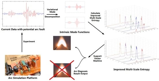
2. Arc Fault Diagnosis Algorithm

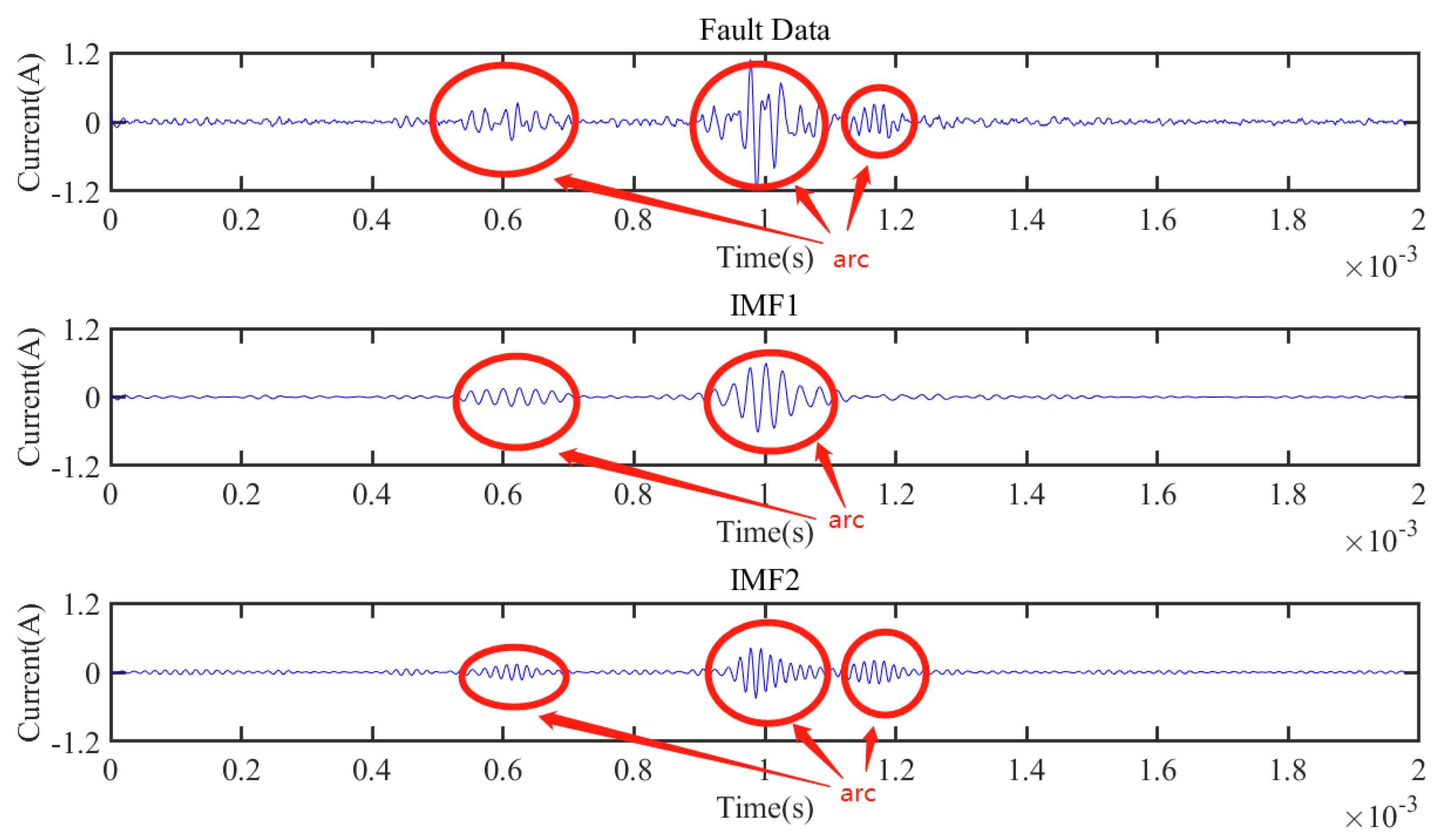
2.1. Arc Fault Data Feature Analysis

The proposed method of our research focused on its application in power stations located in Hubei Enshi Badong. One of them was the Songjialiangzi power plant. Photos of it are shown in Figure 2a,b.

In order to analyze the features of arc fault data, a photovoltaic DC arc generation experiment platform was built. The system chart is shown in Figure 3.

This system consisted of a PV array, a breaker, a load resistance, a current and voltage sampling device, and an arc generator. The sampling device consisted of a Hall current sensor and an oscilloscope. The sampling frequency was 500 kHz. The arc generator was established according to the UL1699B standard, whose structure is shown in Figure 4. The photos of sampling devices, the arc generator, and the arc are shown in Figure 5, Figure 6 and Figure 7.

In the experiment, the knob of the arc generator was slowly rotated to shorten the distance between the electrodes. As the distance became smaller, an arc was generated between the electrodes. Then the oscilloscope collected the current data. The current data of an arc fault under different load conditions was obtained by changing the value of the load resistance. By removing the arc generator, normal current data were also obtained.

The unprocessed signal showed that the low frequency AC noise existed in both normal and arc fault situations. This type of noise does not help to detect the fault and makes the problem complicated. Therefore, a high-pass filter with a cut-off frequency of 30 kHz was used to remove the low frequency noise. The comparison of processed current data is shown in Figure 8 and Figure 9:

Figure 8 shows that in the time domain, the current of the arc fault oscillated wildly compared to normal situations. Figure 9 indicates that the fault current was significantly different from the normal one in the 30–100 kHz band [10]. VMD was used to process the signal with the aim of analyzing the frequency components related to the arc accurately.

2.2. Variational Model Decomposition

VMD decomposes a time-series signal $\mathrm{f}\left(\mathrm{t}\right)$ into $\mathrm{K}$ IMFs. Each IMF has a central frequency. VMD is an optimization problem based on IMF bandwidth minimization. It can be described by Formula (1). In Formula (1), $\mathrm{K}$ is the number of IMFs, $\mathrm{k}$-th IMF is presented by ${\mathrm{u}}_{\mathrm{k}}\left(\mathrm{t}\right)$, the central frequency of ${\mathrm{u}}_{\mathrm{k}}\left(\mathrm{t}\right)$ is presented by ${\mathsf{\omega }}_{\mathrm{k}}$, $\left(\mathrm{a}\ast \mathrm{b}\right)$ represents $\mathrm{a}$ convolved with $\mathrm{b}$. ${||\mathrm{a}||}_2$ represents the L2-norm of $\mathrm{a}$, which can be calculated by Formula (2), and ${\partial }_{\mathrm{t}}\mathrm{X}$ represents the partial derivative of $\mathrm{X}$ with respect to $\mathrm{t}$.

$$\{\begin{array}{l}\underset{\left\{{\mathsf{u}}_{\mathsf{k}}\right\},\left\{{\mathsf{\omega }}_{\mathsf{k}}\right\}}{\mathsf{min}}\left\{{\displaystyle \sum _{\mathsf{k}=1}^{\mathsf{K}}{{\displaystyle \Vert {\partial }_{\mathsf{t}}\left[\left(\mathsf{\delta }\left(\mathsf{t}\right)+\frac{\mathsf{j}}{\mathsf{\pi }\mathsf{t}}\right)\cdot {\mathsf{u}}_{\mathsf{k}}\left(\mathsf{t}\right)\right]{\mathsf{e}}^{-\mathsf{j}{\mathsf{\omega }}_{\mathsf{k}}\mathsf{t}}\Vert }}_2^2}\right\}\\ \mathsf{s}\mathsf{u}\mathsf{b}\mathsf{j}\mathsf{e}\mathsf{c}\mathsf{t}\mathsf{ }\mathsf{to}\mathsf{:}\mathsf{ }{\displaystyle \sum _{\mathsf{k}=1}^{\mathsf{K}}{\mathsf{u}}_{\mathsf{k}}\left(\mathsf{t}\right)=\mathsf{f}(\mathsf{t})}\end{array}$$

(1)

$${{\displaystyle \Vert \mathsf{a}\Vert }}_2=\sqrt{{(\mathsf{Re}(\mathsf{a}))}^2+{(\mathsf{Im}(\mathsf{a}))}^2}$$

(2)

Quadratic penalty term $\mathrm{a}$ and Lagrangian multiplier $\mathsf{\lambda }\left(\mathrm{t}\right)$ are used to transform this problem into a non-constrained problem as shown in Formula (3). $\langle \mathrm{x},\mathrm{y}\rangle$ represents the inner product of $\mathrm{x}$ and $\mathrm{y}$.

$$\mathsf{L}\left(\left\{{\mathsf{u}}_{\mathsf{k}}\right\},\left\{{\mathsf{\omega }}_{\mathsf{k}}\right\},\mathsf{\lambda }\right)=\mathsf{\alpha }{\displaystyle \sum _{\mathsf{k}=1}^{\mathsf{K}}{\Vert {\partial }_{\mathsf{t}}\left[\left(\mathsf{\delta }\left(\mathsf{t}\right)+\frac{\mathsf{j}}{\mathsf{\pi }\mathsf{t}}\right)\cdot {\mathsf{u}}_{\mathsf{k}}\left(\mathsf{t}\right)\right]{\mathsf{e}}^{-\mathsf{j}{\mathsf{\omega }}_{\mathsf{k}}\mathsf{t}}\Vert }_2^2}+{\Vert \mathsf{f}(\mathsf{t})-{\displaystyle \sum _{\mathsf{k}=1}^{\mathsf{K}}{\mathsf{u}}_{\mathsf{k}}\left(\mathsf{t}\right)}\Vert }_2^2+\langle \mathsf{\lambda }(\mathsf{t}),\mathsf{f}(\mathsf{t})-{\displaystyle \sum _{\mathsf{k}}{\mathsf{u}}_{\mathsf{k}}(\mathsf{t})}\rangle$$

(3)

This problem can be solved by using alternating the direction multiplier method (ADMM) until an augmented Lagrange saddle point is found. ${\mathrm{u}}_{\mathrm{k}}$, ${\mathsf{\omega }}_{\mathrm{k}}$_, and $\mathsf{\lambda }$ can be updated by using Formulas (4)–(6). For the convenience of subsequent analysis, Formulas (4)–(6) are given in the frequency domain. In Formulas (4)–(6), ${\mathsf{û}}_{\mathrm{k}}\left(\mathsf{\omega }\right)$ is the $\mathrm{k}$-th IMF, and $\hat{\mathrm{f}}\left(\mathsf{\omega }\right)$ is the Fourier transformation result of the $\mathrm{k}$-th IMF. $\mathsf{\theta }$ is the noise tolerance parameter.

$${\mathsf{u}}_{\mathsf{k}}^{\mathsf{n}+1}(\mathsf{\omega })=\frac{\widehat{\mathsf{f}}(\mathsf{\omega })-{\displaystyle \sum _{\mathsf{i}\ne \mathsf{k}}{\stackrel{⌢}{\mathsf{u}}}_{\mathsf{i}}(\mathsf{\omega })}+\frac{\widehat{\mathsf{\lambda }}(\mathsf{\omega })}{2}}{1+2\mathsf{\alpha }{(\mathsf{\omega }-{\mathsf{\omega }}_{\mathsf{k}})}^2}$$

(4)

$${\mathsf{\omega }}_{\mathsf{k}}^{\mathsf{n}+1}=\frac{{\displaystyle {\int }_0^{\infty }\mathsf{\omega }{\left|{\stackrel{⌢}{\mathsf{u}}}_{\mathsf{k}}(\mathsf{\omega })\right|}^2\mathrm{d}\mathsf{\omega }}}{{\displaystyle {\int }_0^{\infty }{\left|{\stackrel{⌢}{\mathsf{u}}}_{\mathsf{k}}(\mathsf{\omega })\right|}^2\mathrm{d}\mathsf{\omega }}}$$

(5)

$${\widehat{\mathsf{\lambda }}}^{\mathsf{n}+1}(\mathsf{\omega })={\widehat{\mathsf{\lambda }}}^{\mathsf{n}}(\mathsf{\omega })+\mathsf{\theta }\left[\widehat{\mathsf{f}}(\mathsf{\omega })-{\displaystyle \sum _{\mathsf{k}}{\widehat{\mathsf{u}}}_{\mathsf{k}}^{\mathsf{n}+1}(\mathsf{\omega })}\right]$$

(6)

The iteration of ${\mathrm{u}}_{\mathrm{k}}$, ${\mathsf{\omega }}_{\mathrm{k}}$_, and $\mathsf{\lambda }$ can be stopped when an augmented Lagrange saddle point is found, which can be judged by Formula (7):

$$\frac{{\displaystyle \sum _{\mathsf{k}}{\Vert {\widehat{\mathsf{u}}}_{\mathsf{k}}^{\mathsf{n}+1}-{\widehat{\mathsf{u}}}_{\mathsf{k}}^{\mathsf{n}}\Vert }_2^2}}{{\Vert {\widehat{\mathsf{u}}}_{\mathsf{k}}^{\mathsf{n}}\Vert }_2^2}<\mathsf{\epsilon }$$

(7)

When Formula (7) is satisfied, the original signal f(t) has been decomposed into $\mathrm{K}$ IMFs $\left\{{\mathrm{u}}_{\mathrm{k}}\right\}$. The central frequency of ${\mathrm{u}}_{\mathrm{k}}$ is ${\mathsf{\omega }}_{\mathrm{k}}$.

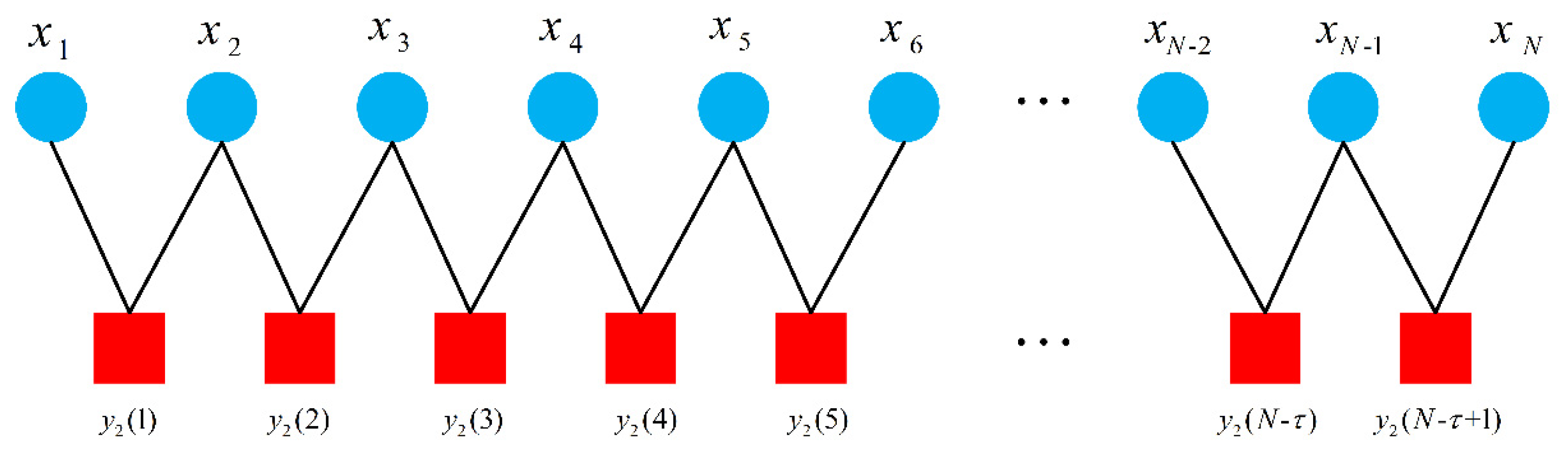
2.3. Multi-Scale Fuzzy Entropy

After $\mathrm{K}$ IMFs are obtained by using VMD, the parameter calculated from the IMFs must be chosen as the feature of the arc. This parameter should basically maintain the same value when an arc fault does not occur. Once an arc fault occurs, this parameter should change noticeably. In this research, IMFE was chosen as the parameter. IMFE is used to measure the complexity of the time-series signal under different scales. It can be calculated through following steps.

Firstly, some sampling points in the original time-series signal were selected by using the sliding window method. Then the selected sampling points sequence {$\mathrm{u}\left(\mathrm{i}\right):1\le \mathrm{i}\le \mathrm{N}$} needed to be coarsened. The coarsened sequence was established by using Formula (8):

$${\mathsf{y}}_{\mathsf{\tau }}(\mathsf{j})=\frac{1}{\mathsf{\tau }}{\displaystyle \sum _{\mathsf{i}=\mathsf{j}}^{\mathsf{j}+\mathsf{\tau }-1}\mathsf{u}(\mathsf{i}),1\le \mathsf{j}\le \mathsf{N}-\mathsf{\tau }+1}$$

(8)

In Formula (8), $\mathsf{\tau }$ represents the length of a factor in the coarsened sequence. This process is illustrated in Figure 10.

Then the coarsened sequence {${\mathrm{y}}_{\mathsf{\tau }}\left(\mathrm{j}\right):\mathsf{ }1\le \mathrm{j}\le \left(\mathrm{N}-\mathsf{\tau }+1\right)$} was converted into a set of vectors {${\mathrm{X}}_{\mathrm{l}}^{\mathrm{m}}:1\le \mathrm{l}\le \left(\mathrm{N}-\mathsf{\tau }-\mathrm{m}+2\right)$}. Formula (9) indicates the specific calculation:

$${\mathsf{X}}_{\mathsf{j}}^{\mathsf{m}}=\{{\mathsf{y}}_{\mathsf{\tau }}(\mathsf{j}),{\mathsf{y}}_{\mathsf{\tau }}(\mathsf{j}+1),\cdots ,{\mathsf{y}}_{\mathsf{\tau }}(\mathsf{j}+\mathsf{m}-1)\}-\overline{{\mathsf{y}}_{\mathsf{\tau }}(\mathsf{j})},\mathsf{j}=1,2,\cdots ,\mathsf{N}-\mathsf{m}-\mathsf{\tau }+2$$

(9)

In Formula (9), $\overline{{\mathrm{y}}_{\mathsf{\tau }}\left(\mathrm{j}\right)}$ can be calculated by using Formula (10):

$$\overline{{\mathsf{y}}_{\mathsf{\tau }}(\mathsf{j})}=\frac{1}{\mathsf{m}}{\displaystyle \sum _{\mathsf{j}\prime =0}^{\mathsf{m}-1}{\mathsf{y}}_{\mathsf{\tau }}(\mathsf{j}+\mathsf{j}\prime )}$$

(10)

The distance d[${\mathrm{X}}_{\mathrm{i}}^{\mathrm{m}},{\mathrm{X}}_{\mathrm{j}}^{\mathrm{m}}$] between ${\mathrm{X}}_{\mathrm{i}}^{\mathrm{m}}$ and ${\mathrm{X}}_{\mathrm{j}}^{\mathrm{m}}$ is defined as the maximum value of the difference between the two corresponding elements:

$$\begin{array}{c}{\mathsf{d}}_{\mathsf{i}\mathsf{j}}^{\mathsf{m}}=\mathsf{d}[{\mathsf{X}}_{\mathsf{i}}^{\mathsf{m}},{\mathsf{X}}_{\mathsf{j}}^{\mathsf{m}}]=\underset{\mathsf{k}\in (0,\mathsf{m}-1)}{\mathsf{max}}\left\{\right|{\mathsf{y}}_{\mathsf{\tau }}(\mathsf{i}+\mathsf{k})-\overline{{\mathsf{y}}_{\mathsf{\tau }}(\mathsf{i})}-({\mathsf{y}}_{\mathsf{\tau }}(\mathsf{j}+\mathsf{k})-\overline{{\mathsf{y}}_{\mathsf{\tau }}(\mathsf{j})})\left|\right\}\\ \mathsf{i},\mathsf{j}=1,2,\cdots ,\mathsf{N}-\mathsf{m}-\mathsf{\tau }+2,\mathsf{i}\ne \mathsf{j}\end{array}$$

(11)

The similarity degree ${\mathrm{D}}_{\mathsf{ij}}^{\mathrm{m}}$ of the vectors ${\mathrm{X}}_{\mathrm{i}}^{\mathrm{m}}$ and ${\mathrm{X}}_{\mathrm{j}}^{\mathrm{m}}$ is defined by a fuzzy function $\mathsf{\mu }\left({\mathrm{d}}_{\mathsf{ij}}^{\mathrm{m}},\mathsf{\beta },\mathrm{r}\right)$. In Formula (12), $\mathrm{r}$ is calculated according to the original data and $\mathsf{\beta }$ is an adjustable constant. $\mathsf{\rho }$ is an adjustment factor used to enhance the ability of noise tolerance.

$${\mathsf{D}}_{\mathsf{i}\mathsf{j}}^{\mathsf{m}}=\mathsf{\mu }({\mathsf{d}}_{\mathsf{i}\mathsf{j}}^{\mathsf{m}},\mathsf{\beta },\mathsf{r})=\{\begin{array}{c}1,0\le {\mathsf{d}}_{\mathsf{i}\mathsf{j}}^{\mathsf{m}}\le \mathsf{\rho }\mathsf{r}\hfill \\ {\mathsf{e}}^{-\mathsf{ln}2{(\frac{{\mathsf{d}}_{\mathsf{i}\mathsf{j}}^{\mathsf{m}}}{\mathsf{r}})}^{\mathsf{\beta }}},{\mathsf{d}}_{\mathsf{i}\mathsf{j}}^{\mathsf{m}}\mathsf{>}\mathsf{\rho }\mathsf{r}\hfill \end{array}$$

(12)

Once a similarity degree is defined, IMFE can be calculated according to Formula (13):

$$\mathsf{F}\mathsf{u}\mathsf{z}\mathsf{z}\mathsf{y}\mathsf{E}\mathsf{n}(\mathsf{m},\mathsf{\beta },\mathsf{r})=\underset{\mathsf{N}\to \infty }{\mathsf{lim}}[\mathsf{ln}{\mathsf{\varphi }}^{\mathsf{m}}(\mathsf{\beta },\mathsf{r})-\mathsf{ln}{\mathsf{\varphi }}^{\mathsf{m}+1}(\mathsf{\beta },\mathsf{r})]$$

(13)

In Formula (13):

$${\mathsf{\varphi }}^{\mathsf{m}}(\mathsf{\beta },\mathsf{r})=\frac{1}{\mathsf{N}-\mathsf{m}}{\displaystyle \sum _{\mathsf{i}=1}^{\mathsf{N}-\mathsf{m}}(\frac{1}{\mathsf{N}-\mathsf{m}-1}{\displaystyle \sum _{\begin{array}{l}\mathsf{j}=1\\ \mathsf{j}\ne \mathsf{i}\end{array}}^{\mathsf{N}-\mathsf{m}}{\mathsf{D}}_{\mathsf{i}\mathsf{j}}^{\mathsf{m}}})}$$

(14)

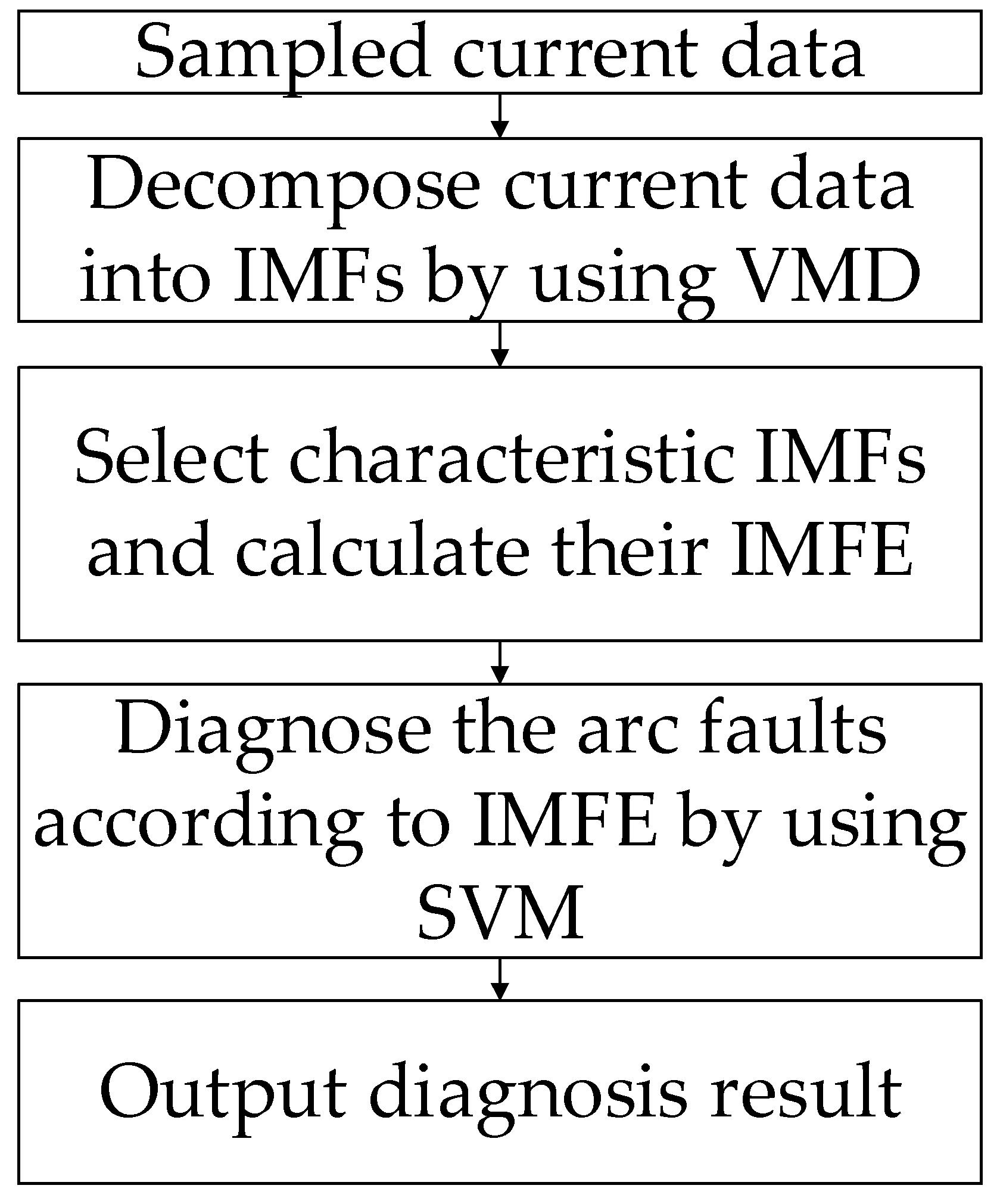
2.4. The Steps of Arc Fault Diagnosis Algorithm

Aiming at the non-linear and non-stationary characteristics of PV DC current, arc diagnosis is particularly suitable for combing VMD and IMFE together. The specific steps of the arc fault diagnosis algorithm are described below.

For the first step, DC current data were decomposed into several IMFs by VMD. Firstly, we initialized the number of IMFs, $\mathrm{K}$ IMF signal set $\left\{{\hat{\mathrm{u}}}_{\mathrm{k}}^1\right\}$, central frequency set $\left\{{\hat{\mathsf{\omega }}}_{\mathrm{k}}^1\right\}$, and Lagrangian ${\hat{\mathsf{\lambda }}}^1$. We set n as 0. We set the value of the quadratic penalty term $\mathrm{a}$. We set the noise tolerance parameter $\mathsf{\theta }$. Then we updated $\left\{{\hat{\mathrm{u}}}_{\mathrm{k}}^1\right\}$, $\left\{{\hat{\mathsf{\omega }}}_{\mathrm{k}}^1\right\}$, and ${\hat{\mathsf{\lambda }}}^1$ by using Formulas (4)–(6) until Formula (7) was satisfied. Eventually the K IMFs $\left\{{\mathrm{u}}_{\mathrm{k}}\right\}$ and the corresponding central frequency $\left\{{\mathsf{\omega }}_{\mathrm{k}}\right\}$ were obtained.

In the second step, based on the wave form of IMFs $\left\{{\mathrm{u}}_{\mathrm{k}}\right\}$, IMFs related to arc faults were selected.

For the third step, we used IMFE to analyze the effective intrinsic mode function. Firstly, we initialized the length of the sliding window $\mathrm{N}$, the length of a factor in the coarsened sequence $\mathsf{\tau }$, the dimension of the converted vector $\mathrm{m}$, the values of the adjustable constants $\mathsf{\rho }$ and $\mathsf{\beta }$, and the formula for calculating $\mathrm{r}$ according to the original data. Then N sampling points from an IMF signal ${\mathrm{u}}_{\mathrm{k}}$ were selected by using a sliding window. The selected sampling points {$\mathrm{u}\left(\mathrm{i}\right):1\le \mathrm{i}\le \mathrm{N}$} were coarsened by using Formula (8). Then the coarsened sequences {${\mathrm{y}}_{\mathsf{\tau }}\left(\mathrm{j}\right):\mathsf{ }1\le \mathrm{j}\le \left(\mathrm{N}-\mathsf{\tau }+1\right)$} were converted into vectors by using Formulas (9) and (10). At last, by defining distance and the similarity degree function of these vectors {${\mathrm{X}}_{\mathrm{l}}^{\mathrm{m}}:1\le \mathrm{l}\le \left(\mathrm{N}-\mathsf{\tau }-\mathrm{m}+2\right)$}, the IMFE could be calculated by using Formulas (13) and (14). By sliding the window forward, IMFE based on IMF could be calculated eventually.

In the final step, we took the IMFE obtained in step 3 and the corresponding labels (normal data were marked as 1, and fault data were marked as 0) of them as the training objectives. These data were used to train the support vector machine. The remaining untrained data were used to verify the training effect of the support vector machine.

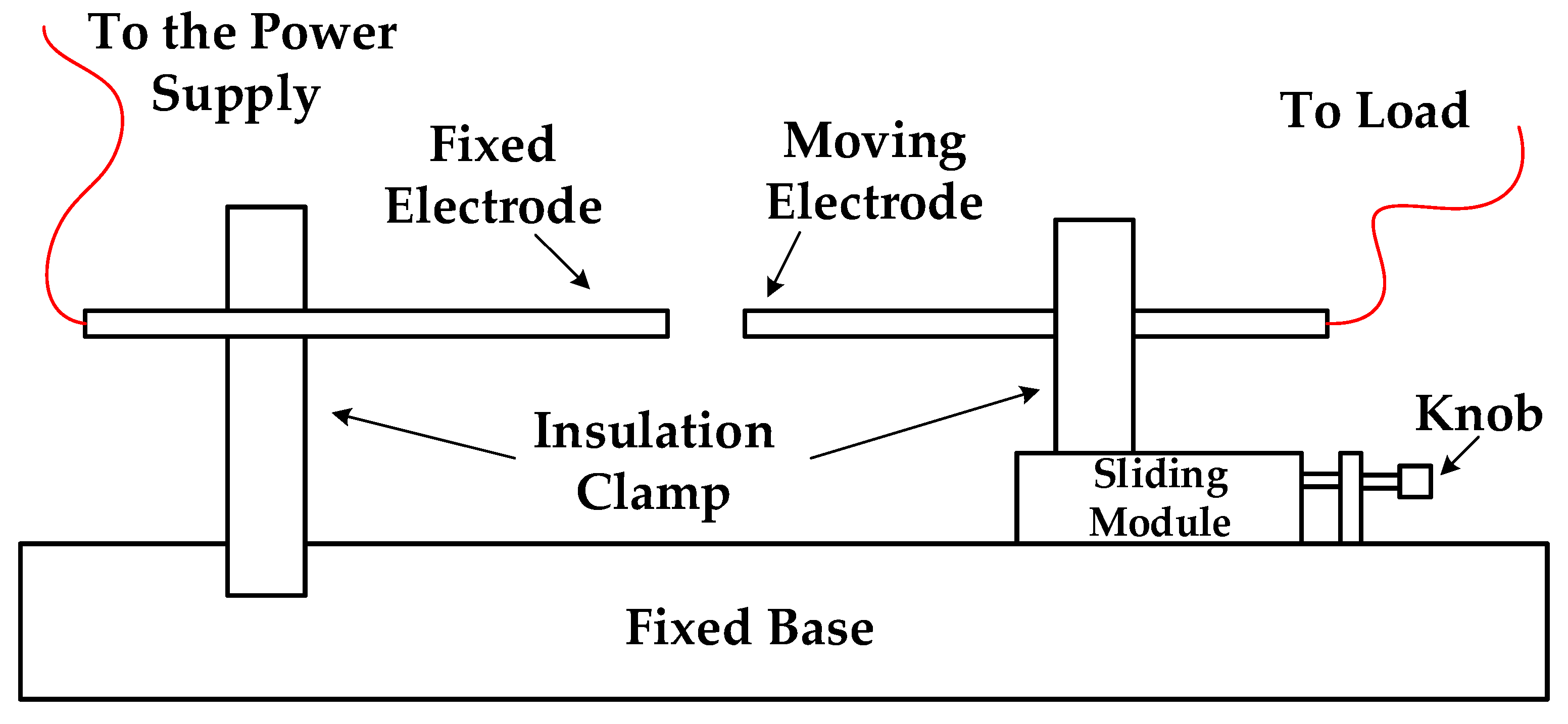
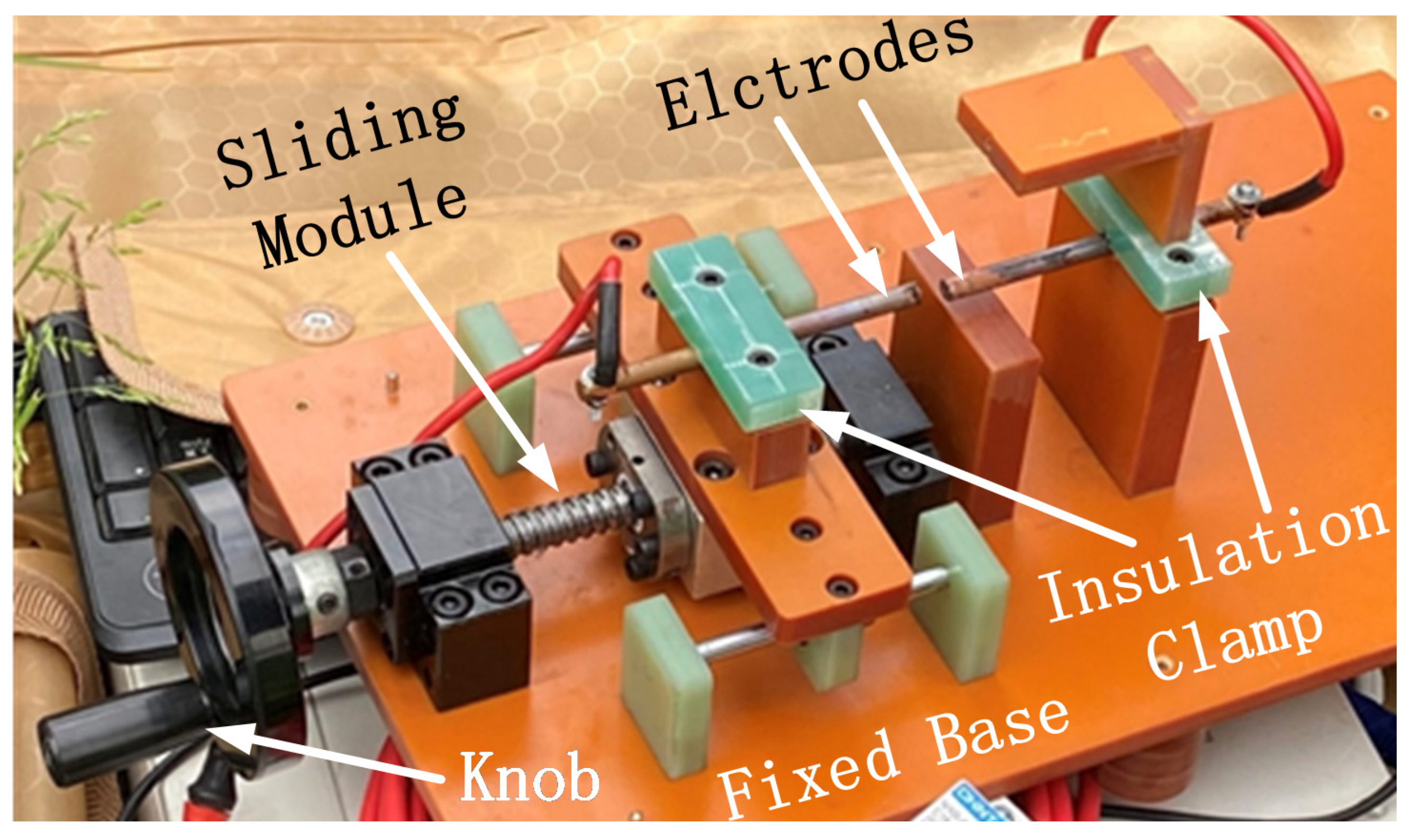
3. The Validation of the Arc Fault Diagnosis Algorithm

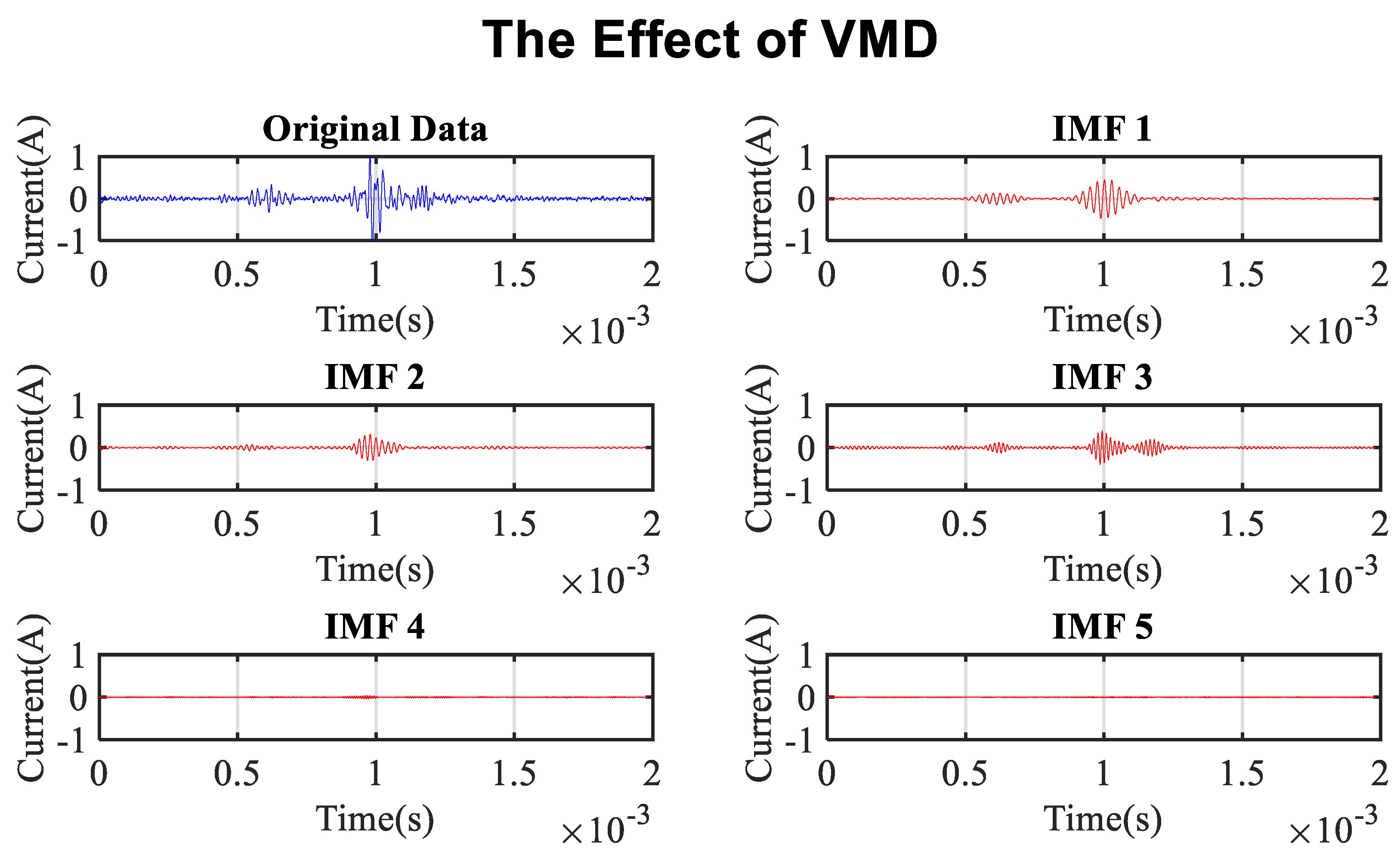
3.1. VMD Parameter Selection

Before performing VMD, the number of decomposed IMFs must be selected. When the K value is small, the decomposed IMFs cannot contain all the information of the original data. When the K value is large, mode mixing will occur between the IMFs, which makes these IMFs distorted signals. Therefore, the selection of the K value is very important.

In this research, the K value was chosen by decomposing the signal several times with different K values. After a set number of iterations with N as 0, set $\left\{{\hat{\mathrm{u}}}_{\mathrm{k}}^1\right\}$, $\left\{{\hat{\mathsf{\omega }}}_{\mathrm{k}}^1\right\}$, and ${\hat{\mathsf{\lambda }}}^1$ as suitable size zero matrix, we set the noise tolerance $\mathsf{\theta }$ as 0.5 and set the quadratic penalty term $\mathrm{a}$ as 2000.

Table 1. K from 1 to 5, the center frequency of IMFs after VMD.

K Value	IMF1	IMF2	IMF3	IMF4	IMF5
K = 1	40.7 kHz	N/A	N/A	N/A	N/A
K = 2	39.3 kHz	64.1 kHz	N/A	N/A	N/A
K = 3	39.3 kHz	64.1 kHz	122.4 kHz	N/A	N/A
K = 4	39.3 kHz	64.1 kHz	121.9 kHz	179.3 kHz	N/A
K = 5	37.9 kHz	48.8 kHz	65.8 kHz	123.3 kHz	193.9 kHz

shows the results of decomposition when K varies from 1 to 5.

As shown in Table 1, IMF1 and IMF2 have relatively close central frequencies when K = 5. Mode mixing may occur in this situation. In order to decide whether 4 or 5 is the appropriate K value, the IMFs when K is 4 and 5 are shown in Figure 11, Figure 12, Figure 13 and Figure 14.

Figure 14 indicates that IMF1, IMF2, and IMF3 had an obvious overlapping part in the frequency domain. This phenomenon indicates that from the perspective of avoiding mode mixing, K = 4 was a more appropriate choice than K = 5.

Except for mode mixing, the stability of the results can also be the criterion for choosing the K value.

Table 2. K = 4, the center frequency of IMFs after VMD of multiple sets of data.

Type	Label	IMF1	IMF2	IMF3	IMF4
normal	1	42.2 kHz	64.5 kHz	125.6 kHz	187.1 kHz
normal	2	41.7 kHz	65.0 kHz	124.3 kHz	190.4 kHz
normal	3	42.8 kHz	64.1 kHz	125.2 kHz	179.5 kHz
fault	1	42.2 kHz	64.7 kHz	126.7 kHz	188.1 kHz
fault	2	42.1 kHz	66.8 kHz	124.1 kHz	186.6 kHz
fault	3	42.6 kHz	64.3 kHz	123.8 kHz	183.9 kHz

and

Table 3. K = 5, the center frequency of IMFs after VMD of multiple sets of data.

Type	Label	IMF1	IMF2	IMF3	IMF4	IMF5
normal	1	42.2 kHz	64.1 kHz	95.7 kHz	127.5 kHz	187.4 kHz
normal	2	41.7 kHz	64.8 kHz	105.2 kHz	156.1 kHz	203.0 kHz
normal	3	42.9 kHz	63.9 kHz	110.9 kHz	160.7 kHz	210.0 kHz
fault	1	40.6 kHz	55.4 kHz	66.9 kHz	128.9 kHz	188.2 kHz
fault	2	40.9 kHz	57.6 kHz	68.1 kHz	124.5 kHz	186.7 kHz
fault	3	41.8 kHz	60.7 kHz	69.1 kHz	123.8 kHz	163.8 kHz

show the central frequencies of the IMFs decomposed from several sets of data when K was set as either 4 or 5.

Table 2 and Table 3 indicate that the stability when K = 4 was better than the stability when K = 5. Therefore, from the perspectives of stability and mode mixing, K should be set as 4 in this research.

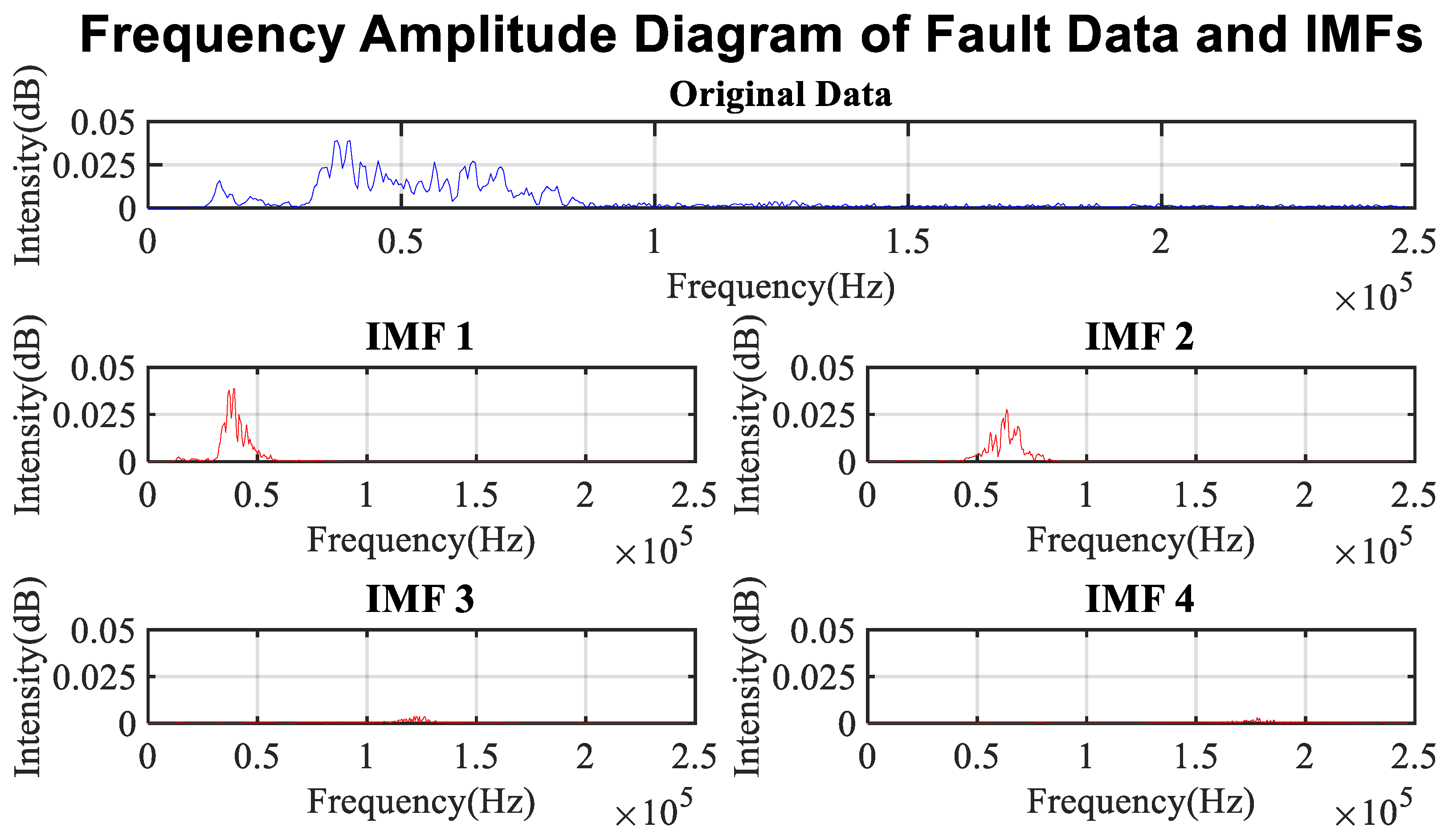
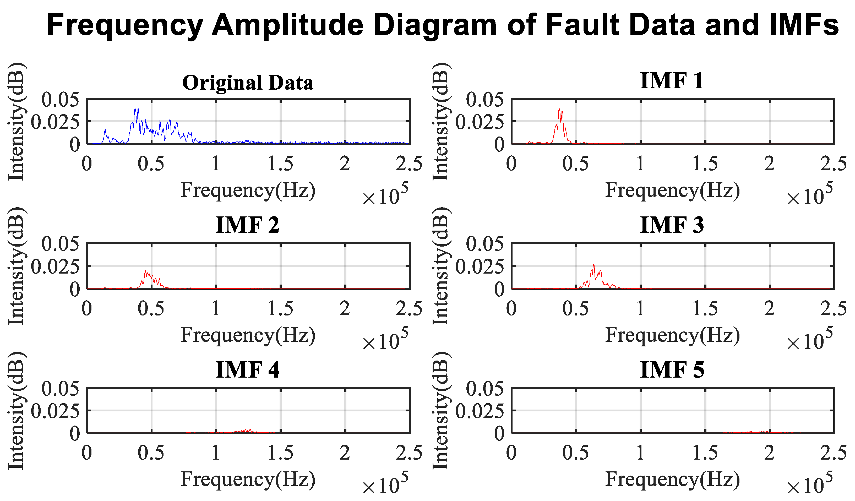
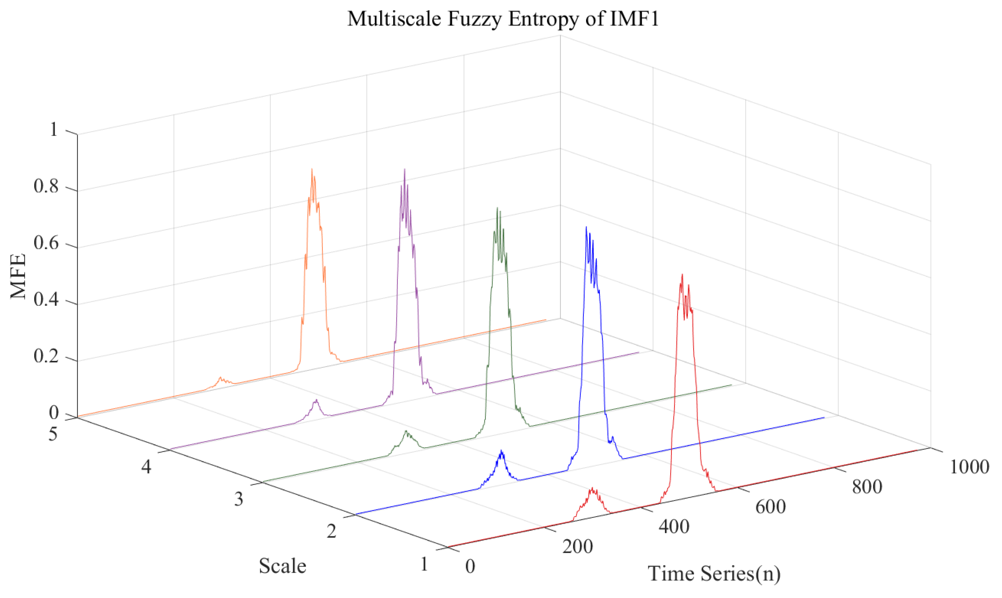
3.2. Selection of IMF and Calculation of IMFE

Figure 9 indicates that the frequency bandwidth related to arc faults ranges from 30 kHz to 100 kHz. Figure 12 illustrate that when K = 4, IMF1 and IMF2 are in this bandwidth. In addition, Figure 15 shows that once the current fluctuates wildly because an arc fault occurs, IMF1 and IMF2 will fluctuate synchronously. Therefore, IMF1 and IMF2 should be chosen as the IMFs related to the arc fault.

As proposed in Section 2.3, the IMFEs of these 2 IMFs were calculated. The length of the sliding window, which is represented by $\mathrm{N}$, was chosen as 20. The length of a factor in the coarsened sequence, which is represented by $\mathsf{\tau }$, was less than or equal to 5. The dimension of vectors converted from the coarsened sequence, which is represented by $\mathrm{m}$, was 3. As for parameters in the similarity degree function, $\mathsf{\rho }=1$, $\mathsf{\beta }=2$, $\mathrm{r}$ is calculated by Formula (15), and $\mathrm{S}$ is the standard deviation of all the original data. The IMFEs calculated from IMF1 and IMF2 are shown in Figure 16 and Figure 17.

$$\mathsf{r}=0.15\cdot \mathsf{S}$$

(15)

By combining Figure 15, Figure 16 and Figure 17, the IMFE successfully met the requirement of the features of arc diagnosis. The value of IMFE was close to 0 when an arc fault did not happen. Once an arc fault occurred, the value of IMFE increased noticeably, and the magnitude was proportional to the severity of the arc fault.

Before conducting validation, the choices of $\mathsf{\tau }$ and N need to be discussed. The IMFE calculation above was conducted when $\mathsf{\tau }$ was less than 5. When the length of the sliding window and the length of the factor are chosen differently, the result could be different.

Figure 18 shows the average IMFE-scale curve when the length of the sliding window is chosen as 100, 75, or 50. The IMFE is calculated from IMF1 in Figure 18.

Figure 18 indicates that when the N chosen is larger, the average IMFE is larger. This means that the fluctuation in IMFE caused by an arc is stronger when the chosen N is larger. However, a larger length of the sliding window will make the calculation more time-consuming. In Figure 16 and Figure 17, N is set as 20. The fluctuation is still strong enough for arc detection. Therefore, N should be chosen based on computing power and speed needs.

Regardless of N, the average IMFE always decays to a small value when $\mathsf{\tau }$ is equal to 10. A possible explanation can be stated as the following: in the IMF1 which IMFE is calculated from, the arc portion counts for the same number of data points regardless of the value of N. When the chosen $\mathsf{\tau }$ is larger than the number of arc fault data points, the IMFEs which contain arc data points are reduced by the presence of normal data points, which can cause the arc to go undetected based on IMFE. Therefore, the IMFE of a small $\mathsf{\tau }$ value will make sure that an arc with short bandwidth can be detected. If fluctuations on the IMFE exists, the larger the $\mathsf{\tau }$ of IMFE is, and the wider the bandwidth of the arc is.

3.3. Fault Diagnosis and Validation

In order to validate the algorithm, 5100 current sampling points were obtained from the experimental platform proposed in Section 2.1. In this process, 24 experiments, including 12 normal experiments and 12 arc fault experiments with different load resistances, were carried out. SVM was used to detect the arc fault based on the IMFEs of IMF1 and IMF2. Therefore, these data were divided into a training set and a verification set. The training set contains 70% of the data while the verification set contains the rest.

The SVM program used in this paper was the LibSVM program provided by Chang Chih-Chung and Lin Chih-Jen [41]. The radial basis function was selected as the kernel function of the SVM, and the particle swarm optimization (PSO) algorithm was used to optimize the penalty parameter $\mathrm{c}$ and the kernel function parameter $\mathrm{g}$ of the SVM.

The diagnosis result type can be divided into TP (true positive, an arc fault sample was diagnosed as an arc fault sample), FP (false positive, a normal sample was diagnosed as an arc fault sample), TN (true negative, a normal sample was diagnosed as a normal sample) and FN (false negative, an arc fault sample was diagnosed as a normal sample). From the definitions of these result types, FP and FN were the wrong diagnosis results and the others were the right diagnosis results.

The 1530 samples in the validation set were diagnosed by SVM and the results are shown in

Table 4. SVM Training Effects.

Result Type	TP	FP	TN	FN	Total
Number	985	11	529	5	1530
Percentage	64.4%	0.7%	34.6%	0.3%	100%

. Table 4 illustrates that the proposed arc fault diagnosis algorithm had a great effect on detecting arc faults. Of the 1530 samples, 1514 were diagnosed correctly. The accuracy of this algorithm was 99.0% on this validation data set.

4. Conclusions

This research proposed a fault diagnosis method based on VMD, IMFE, and SVM for PV arc diagnosis. An experimental platform was established to obtain the training and validation current data. During the arc diagnosis, the current data were first decomposed into several IMFs by using VMD. Then the IMFs related to an arc were picked for IMFE calculation. After IMFEs of these IMFs were obtained, they were used as the input of SVM to detect the arc fault. According to the results of validation, the proposed arc fault diagnosis method could be used to detect an arc fault based on current data and was relatively accurate.

The advantages of this method can be stated as follows: using VMD makes sure that the decomposed signals have a central frequency and limited frequency bandwidth; by choosing an appropriate K value, mode mixing can be avoided, and IMFs are guaranteed to make sense; compared to other decomposition methods, the result of VMD contains relatively rich information, which is beneficial to the subsequent analysis. Using IMFE successfully converts fluctuation in IMFs into amplitude change in IMFEs, which makes using SVM possible. Compared to developed methods, the advantages of the proposed method can be stated as follows: compared to using sensors to detect the arc [42], the proposed method only requires users to add sampling devices to the scene. High sampling rate devices can be chosen with same investment. Fewer devices needing to be installed also makes the proposed method easy to apply in different situations. Compared to using thermal imaging [43], the proposed method can significantly save on the cost of equipment installation. The proposed method is also more universal than thermal imaging. Compared to other frequency-domain methods [44], this method avoids the choice of functions such as wavelet basis, window functions, etc. By decreasing the length of the sliding window, the calculation speed of the proposed method can be improved, though the significance of the results may be weakened at the same time. Users can find a proper balance between them based on the requirements of the actual application. Furthermore, this algorithm has potential application in bearing fault diagnosis, mechanical fault analysis of circuit breakers, multi-level inverter analysis, and so on.

However, compared to using sensors and thermal imaging, accuracy may be a disadvantage of the proposed method. The rapidity of the proposed algorithm was not validated in this research. It is possible that an integrated online arc fault diagnostic device could be established based on this algorithm.

References

1. PVPS; Kaizuka, I.; Jäger, W.A. Snapshot of Global PV Markets. 2020. Available online: https://www.researchgate.net/publication/324728482_2017_SNAPSHOT_OF_GLOBAL_PHOTOVOLTAIC_MARKETS (accessed on 8 July 2021).
2. Taylor, M.; Ralon, P.; Ilas, A. The Power to Change: Solar and Wind Cost Reduction Potential to 2025. International Renewable Energy Agency, 2016; p. 3. Available online: https://www.irena.org/publications/2016/Jun/The-Power-to-Change-Solar-and-Wind-Cost-Reduction-Potential-to-2025 (accessed on 8 July 2021).
3. Hossam, A.A.; Ahmed, E.E.; Ibrahim, B.M.T. A new monitoring technique for fault detection and classification in PV systems based on rate of change of voltage-current trajectory. Int. J. Electr. Power Energy Syst. 2021, 133. [Google Scholar] [CrossRef]
4. Shi, Y.; Sun, Y.; Liu, J.; Du, X. Model and stability analysis of grid-connected PV system considering the variation of solar irradiance and cell temperature. Int. J. Electr. Power Energy Syst. 2021, 132. [Google Scholar] [CrossRef]
5. Jiang, Y.; Kang, L.; Liu, Y. The coordinated optimal design of a PV-battery system with multiple types of PV arrays and batteries: A case study of power smoothing. J. Clean. Prod. 2021, 310. [Google Scholar] [CrossRef]
6. Haffaf, A.; Lakdja, F.; Abdeslam, D.O.; Meziane, R. Monitoring, measured and simulated performance analysis of a 2.4 kWp grid-connected PV system installed on the Mulhouse campus, France. Energy Sustain. Dev. 2021, 62, 44–55. [Google Scholar] [CrossRef]
7. Houssein, E.H.; Mahdy, M.A.; Fathy, A.; Rezk, H. A modified Marine Predator Algorithm based on opposition based learning for tracking the global MPP of shaded PV system. Expert Syst. Appl. 2021, 183. [Google Scholar] [CrossRef]
8. Yurtseven, K.; Karatepe, E.; Deniz, E. Sensorless fault detection method for photovoltaic systems through mapping the inherent characteristics of PV plant site: Simple and practical. Sol. Energy 2021, 216, 96–110. [Google Scholar] [CrossRef]
9. Shapiro, F.R.; Radibratovic, B. DC arc flash hazards and protection in photovoltaic systems. In Proceedings of the 2013 IEEE 39th Photovoltaic Specialists Conference (PVSC), Tampa Bay, FL, USA, 16–21 June 2013. [Google Scholar]
10. Lu, S.; Phung, B.T.; Zhang, D. A comprehensive review on DC arc faults and their diagnosis methods in photovoltaic systems. Renew. Sustain. Energy Rev. 2018, 89, 88–98. [Google Scholar] [CrossRef]
11. Dhar, S.; Patnaik, R.K.; Dash, P.K. Fault detection and location of photovoltaic based DC microgrid using differential protection strategy. IEEE Trans Smart Grid 2018, 9, 4303–4312. [Google Scholar] [CrossRef]
12. Mu, L.; Wang, Y.; Jiang, W.; Zhang, F. Study on characteristics and detection method of DC arc fault for photovoltaic system. Proc. CSEE 2016, 36, 5236–5244. [Google Scholar]
13. Lu, S.; Ma, R.; Sirojan, T.; Phung, B.T.; Zhang, D. Lightweight transfer nets and adversarial data augmentation for photovoltaic series arc fault detection with limited fault data. Int. J. Electr. Power Energy Syst. 2021, 130. [Google Scholar] [CrossRef]
14. Humbert, J.B.; Schweitzer, P.; Weber, S. Serial-arc detection by use of Spectral Dispersion Index (SDI) analysis in a low-voltage network (270V HVDC). Electr. Power Syst. Res. 2021, 196. [Google Scholar] [CrossRef]
15. Chen, S.; Li, X.; Meng, Y.; Xie, Z. Wavelet-based protection strategy for series arc faults interfered by multicomponent noise signals in grid-connected photovoltaic systems. Sol. Energy 2019, 183, 327–336. [Google Scholar] [CrossRef]
16. Goodman, M. How ultrasound can detect electrical discharge non-invasively and help eliminate arc flash incidents. In Proceedings of the 2007 Electrical Insulation Conference and Electrical Manufacturing Expo, Nashville, TN, USA, 22–24 October 2007. [Google Scholar]
17. Panetta, S. Design of arc Flash protection system using solid state switch, photo detection, with parallel impedance. In Proceedings of the 2013 IEEE IAS Electrical Safety Workshop, Dallas, TX, USA, 11–15 March 2013. [Google Scholar]
18. Restrepo, C.E. Arc Fault detection and discrimination methods. In Electrical Contacts-2007. In Proceedings of the 53rd IEEE Holm Conference on Electrical Contacts, Pittsburgh, PA, USA, 16–19 September 2007. [Google Scholar]
19. Xiong, Q.; Ji, S.; Zhu, L.; Zhong, L.; Liu, Y. A novel DC arc fault detection method based on electromagnetic radiation signal. IEEE Trans. Plasma Sci. 2017, 45, 472–478. [Google Scholar] [CrossRef]
20. Guo, S.Y.; Jones III, J.L.; Dooley, A.S. DC arc Detection and Prevention Circuit and Method. U.S. Patent 6,683,766 B1, 27 January 2004. [Google Scholar]
21. Zhen, M.; Li, W.; Qiang, G.S. The characteristics of DC arc faults current. In Proceedings of the 2013 15th European Conference on Power Electronics and Applications (EPE), Lille, France, 2–6 September 2013. [Google Scholar]
22. Yao, X.; Herrera, L.; Ji, S.; Zou, K.; Wang, J. Characteristic study and time-domain discrete-wavelet-transform based hybrid detection of series DC arc faults. IEEE Trans. Power Electron. 2014, 29, 3103–3115. [Google Scholar] [CrossRef]
23. Chae, S.; Park, J.; Oh, S. Series DC Arc fault detection algorithm for DC microgrids using relative magnitude comparison. IEEE Trans. Emerg. Sel. Top. Power Electron. 2016, 4, 1270–1278. [Google Scholar] [CrossRef]
24. Aarstad, C.; Taufik, T.; Kean., A. Development of arc fault interrupter laboratory testing for low voltage DC electricity. In Proceedings of the 2016 International Seminar on Intelligent Technology and Its Applications (ISITIA), Lombok, Indonesia, 28–30 July 2016. [Google Scholar]
25. Chen, S.; Li, X.; Xiong, J. Series arc fault identification for photovoltaic system based on time-domain and time-frequency-domain analysis. IEEE J. Photovolt. 2017, 7, 1105–1114. [Google Scholar] [CrossRef]
26. Chen, S.; LI, X. PV series arc fault recognition under different working conditions with joint detection method. In Proceedings of the 2016 IEEE 62nd Holm Conference on Electrical Contacts (Holm), Clearwater Beach, FL, USA, 9–12 October 2016. [Google Scholar]
27. He, C.; Mu, L.; Wang, Y. The detection of parallel arc fault in photovoltaic systems based on a mixed criterion. IEEE J. Photovolt. 2017, 7, 1717–1724. [Google Scholar] [CrossRef]
28. Zhu, H.; Wang, Z.; Balog, R.S. Real time arc fault detection in PV systems using wavelet decomposition. In Proceedings of the 2016 IEEE 43rd Photovoltaic Specialists Conference (PVSC), Portland, OR, USA, 5–10 June 2016. [Google Scholar]
29. Yusof MF, M.; Kamaruzaman, M.A.; Ishak, M.; Ghazali, M.F. Porosity detection by analyzing arc sound signal acquired during the welding process of gas pipeline steel. Int. J. Adv. Manuf. Technol. 2017, 89, 3661–3670. [Google Scholar] [CrossRef] [Green Version]
30. Thomas, S.R.; Kurupath, V.; Nair, U. A passive islanding detection method based on K-means clustering and EMD of reactive power signal. Sustain. Energy Grids Netw. 2020, 23. [Google Scholar] [CrossRef]
31. Dibaj, A.; Hassannejad, R.; Ettefagh, M.M.; Ehghaghi, M.B. Incipient fault diagnosis of bearings based on parameter-optimized VMD and envelope spectrum weighted kurtosis index with a new sensitivity assessment threshold. ISA Trans. 2021, 114, 413–433. [Google Scholar] [CrossRef]
32. Li, H.; Liu, T.; Wu, X.; Chen, Q. An optimized VMD method and its applications in bearing fault diagnosis. Measurement 2020, 166. [Google Scholar] [CrossRef]
33. Sukriti; Chakraborty, M.; Mitra, D. Epilepsy seizure detection using kurtosis based VMD’s parameters selection and bandwidth features. Biomed. Signal Process. Control 2021, 64. [Google Scholar]
34. Zhu, S.; Xia, H.; Peng, B.; Zio, E.; Wang, Z.; Jiang, Y. Feature extraction for early fault detection in rotating machinery of nuclear power plants based on adaptive VMD and Teager energy operator. Ann. Nucl. Energy 2021, 160. [Google Scholar] [CrossRef]
35. Wang, Y.; Kiziltas, A.; Blanchard, P.; Walsh, T.R. Calculation of 1D and 2D densities in VMD: A flexible and easy-to-use code. Comput. Phys. Commun. 2021, 266. [Google Scholar] [CrossRef]
36. Shi, G.; Qin, C.; Tao, J.; Liu, C. A VMD-EWT-LSTM-based multi-step prediction approach for shield tunneling machine cutterhead torque. Knowl. Based Syst. 2021. [Google Scholar] [CrossRef]
37. Pincus, S. Approximate entropy (ApEn) as a complexity measure. Chaos 1995, 5, 110–117. [Google Scholar] [CrossRef]
38. Richman, J.S.; Moorman, J.R. Physiological time-series analysis using approximate entropy and sample entropy. Am. J. Physiol. Heart Circ. 2000, 278, 2039–2049. [Google Scholar] [CrossRef] [PubMed] [Green Version]
39. Xie, H.B.; He, W.X.; Liu, H. Measuring time series regularity using nonlinear similarity-based sample entropy. Mod. Phys. Lett. 2008, 372, 7140–7146. [Google Scholar] [CrossRef]
40. Chen, W.; Zhuang, J.; Yu, W.; Wang, Z. Measuring complexity using FuzzyEn, ApEn, and SampEn. Med. Eng. Phys. 2008, 31, 61–68. [Google Scholar] [CrossRef]
41. Chang, C.C.; Lin, C.J. Libsvm. ACM Trans. Intell. Syst. Technol. 2011, 2, 1–27. [Google Scholar] [CrossRef]
42. Luna, B.V.; Monroy-Morales, J.L.; Madrigal Martínez, M.; Torres-Lucio, D.; Weber, S.; Schweitzer, P. Analysis of Internal Signal Perturbations in DC/DC and DC/AC Converters under Arc Fault. Energies 2021, 14, 3005. [Google Scholar] [CrossRef]
43. Glowacz, A. Ventilation Diagnosis of Angle Grinder Using Thermal Imaging. Sensors 2021, 21, 2853. [Google Scholar] [CrossRef] [PubMed]
44. Kim, J.-C.; Kwak, S.-S. Frequency-Domain Characteristics of Series DC Arcs in Photovoltaic Systems with Voltage-Source Inverters. Appl. Sci. 2020, 10, 8042. [Google Scholar] [CrossRef]
Figure 1. Block diagram of the proposed diagram.
Energies 14 04137 g001
Figure 2. Photos of the Songjialiangzi power plant: (a) Frontal view; (b) Side view. (Writings in the figure are not relevant to the meaning of the figure).
Energies 14 04137 g002
Figure 3. The experimental platform.
Energies 14 04137 g003
Figure 4. Structure of the arc generator.
Energies 14 04137 g004
Figure 5. Photo of the arc generator.
Energies 14 04137 g005
Figure 6. Photos of the sampling devices: (a) oscilloscope; (b) Hall current sensor.
Energies 14 04137 g006
Figure 7. Photo of the arc.
Energies 14 04137 g007
Figure 8. The comparison of current waveforms in the time-domain.
Energies 14 04137 g008
Figure 9. The comparison of current waveforms in the frequency-domain.
Energies 14 04137 g009
Figure 10. Schematic diagram of the improved multi-scale fuzzy entropy algorithm.
Energies 14 04137 g010
Figure 11. The waveform of IMFs when K = 4.
Energies 14 04137 g011
Figure 12. Spectrogram of IMFs when K = 4.
Energies 14 04137 g012
Figure 13. The waveform of IMFs when K = 5.
Energies 14 04137 g013
Figure 14. Spectrogram of IMFs when K = 5.
Energies 14 04137 g014
Figure 15. The observed arc part of original data, IMF1 and IMF2.
Energies 14 04137 g015
Figure 16. IMFE under different scales of IMF1.
Energies 14 04137 g016
Figure 17. IMFE under different scales of IMF2.
Energies 14 04137 g017
Figure 18. Average IMFE-scale curve when N = 100, 75, or 50.
Energies 14 04137 g018