Reinforcement Learning Based Peer-to-Peer Energy Trade Management Using Community Energy Storage in Local Energy Market

Abstract

Many studies have proposed a peer-to-peer energy market where the prosumers’ actions, including energy consumption, charge and discharge schedule of energy storage systems, and transactions in local energy markets, are controlled by a central operator. In this paper, prosumers’ actions are not controlled by an operator, and the prosumers freely participate in the local energy market to trade energy with other prosumers. We designed and modeled a local energy market with a management algorithm that uses community energy storage for prosumers who competitively participate in trade in the real-time energy market. We propose an energy-trade management algorithm that manages the trades of prosumers in two phases based on bids and offers submitted by prosumers. The first phase is to manage the trade of prosumers who have submitted fair prices to trade with other prosumers in the real-time energy market. The second phase is managing the trade of prosumers that could not trade in the first phase. Community energy storage is employed in the second phase and controlled by a reinforcement learning-based trading algorithm to decide whether to buy, sell, or do nothing with the prosumers. The action of buying and selling means charging and discharging the community energy storage, respectively. Numerical results show that the proposed trading algorithm gains a near-maximum profit. Besides, we verified that community energy storage yields more profit than the battery wear-out cost.

1. Introduction

The greenhouse gases, which are the most significant driver of global warming, mainly originate from the use of fossil fuels. In 2018, 75% of greenhouse gases were emitted by fossil fuel combustion, and most of them are used in our daily lives, for example, for transportation, energy generation, and industrial use [1,2]. To reduce the amount of greenhouse gas emission, renewable energy sources (RES), including wind, solar, geothermal, and biomass energies, are gaining attention as alternatives to replace fossil fuels. In 2018, worldwide investments in renewable energy amounted to $272.9 billion, and such large investments in RES have affected consumers [3]. Many consumers have installed private RES-generation facilities with government support to lower their electricity bills through self-generation and self-consumption and make profits by selling the surplus energy. Many consumers have become prosumers who can produce energy independently. However, it is difficult for most prosumers to earn a profit by trading with the utility company due to the low feed-in tariff. This led prosumers to create an independent local energy market (LEM) where prosumers can sell their energy to their neighbors. For example, a Dutch company called Vandebron was established in 2014 to provide the first online peer-to-peer (P2P) energy trading, and in the UK, an open utility has launched in 2015 as a pilot program for P2P-trading services [4]. In the USA, the first solar energy sale between neighbors was recorded in Brooklyn, New York, in 2016 [5].

The P2P energy trade gives prosumers an option to trade not only with the utility company but also with other prosumers. The challenge that arises in the P2P energy trade is finding a proper bidding strategy to gain profit. Prosumers have to decide the proper bidding price at the proper time when they need to trade energy according to their demand. If prosumers fail to trade energy, they have to trade with the utility at a low price. There is also an option of adopting an energy storage system (ESS) for time-flexible trading with prosumers, but it is difficult to make profits considering the high battery wear-out cost (BWC). Several studies have demonstrated the economic effects of adopting ESS, and in most cases, it was difficult to make profits without government aid [6].

Herein, we adopt the concept of sharing ESS with nearby local prosumers, known as community energy storage (CES), in LEM to reduce the maintenance cost of ESS. CES can also be used for demand-side management [7], but herein, it is used for prosumers. CES is managed by an energy-trade supporter (ETS) who oversees the trade of prosumers. In our proposed LEM, prosumers submit their bids and offers to ETS, and the ETS decides whether to use CES for prosumers. ETS manages the trade of prosumers in two phases. The first phase is real-time arbitrage trading, and the second phase is reinforcement learning (RL)-based arbitrage trading. In the real-time arbitrage trading phase, the ETS trades with prosumers according to their bids and offers. Prosumer’s energy is transferred from the seller to the buyer according to ETS, so CES is not used in this phase. In the second phase, the ETS decides whether to trade with a prosumer who failed to trade in the first phase. The ETS decides whether to buy, sell, or do nothing. If the ETS decides to buy energy from a prosumer, the energy is stored in CES, and if the ETS decides to sell energy to a prosumer, the energy stored in CES is discharged to the buyer. Notably, the stored energy in CES is only sold to prosumers in the second phase. The ETS chooses its action through an RL-based algorithm that focuses on maximizing its arbitrage trading profit. The key contributions of this work are as follows:

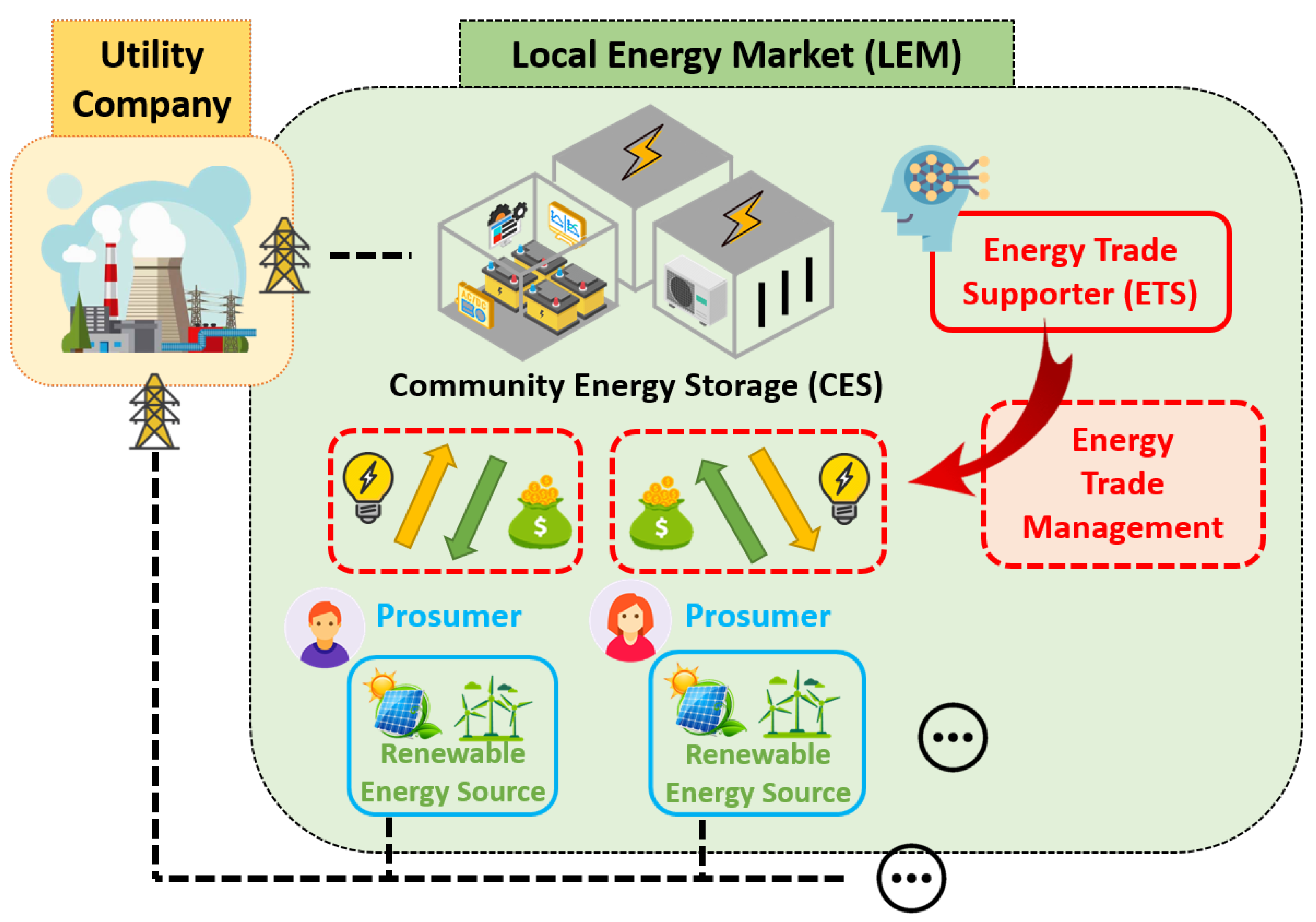
• We designed an LEM where prosumers are not controlled by a central operator. Prosumers freely participate in the LEM, and the trade between prosumers is managed based on the bids and offers submitted by prosumers.
• We proposed a new role called ETS that manages trades in the LEM. ETS not only acts as a middleman between prosumers but also as a supporter for prosumers who failed to trade in real-time LEM.
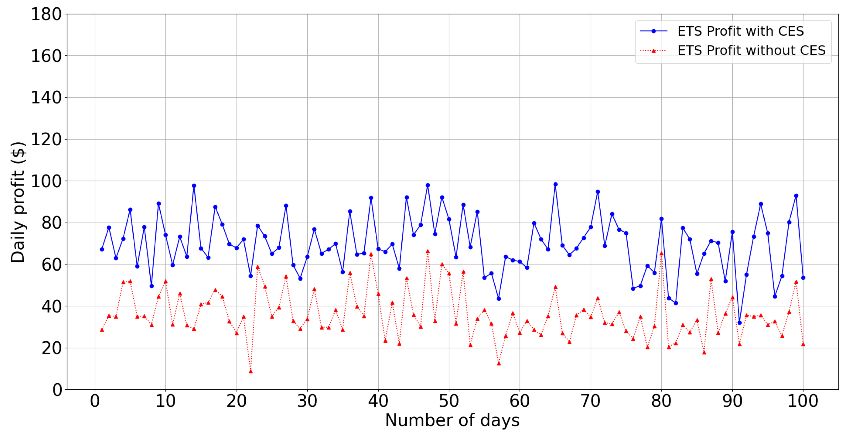
• CES is applied to the LEM and controlled by ETS. CES is used only for prosumers who failed to trade in real-time LEM. Through numerical simulations, we showed that the limited use of CES has more economic benefits than using the CES for all prosumers.
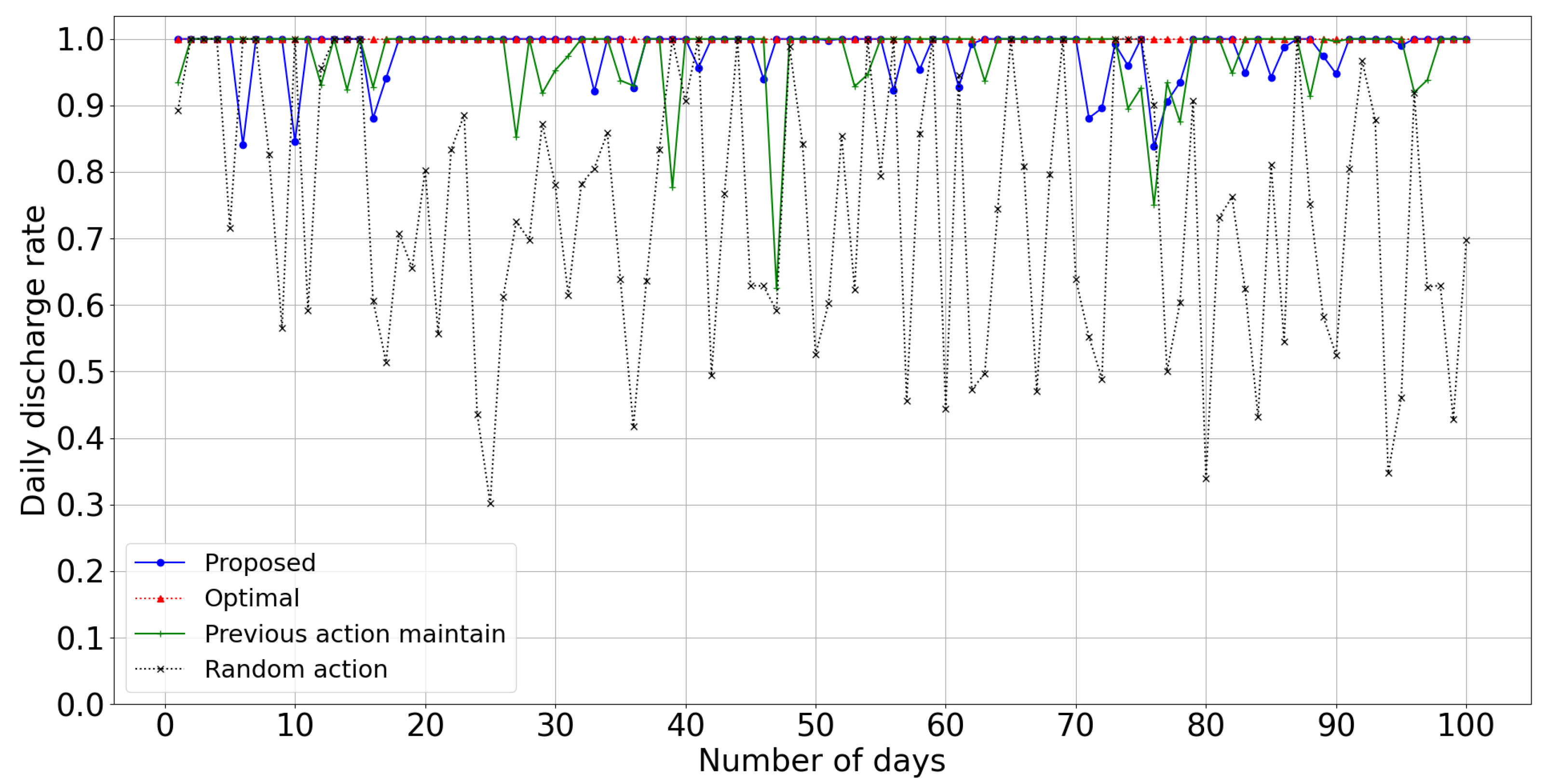
• We adopted an RL-based energy trade management technique for CES, which targets maximizing the trading profit considering BWC. We compared the BWC and economic benefits of CES from the RL-based energy trade management algorithm.

The rest of this paper is organized as follows: Section 2 provides an overview of the recent research on energy trade management systems; Section 3 presents the LEM market design; Section 4 presents the proposed energy trade management algorithm; Section 5 provides the numerical results of the proposed algorithm; Section 6 summarizes the key results of this study.

2. Related Work

We categorize previous studies on energy trade management in LEM into three types: transactive energy management system (EMS), P2P energy trade system, and energy trade system with CES.

2.1. Transactive EMS

The demand response (DR) is a demand-side management technique that attempts to change the energy usage pattern of consumers in response to changing the price or giving incentives [8]. The term transactive energy is being said as a generalized form of DR that focuses on balancing supply and demand by incentivizing prosumers [9]. In transactive energy, the distributed energy resources of prosumers are controlled by their owners, but the transaction mechanism is designed in a system-friendly manner.

In [10,11,12], a transactive EMS that considers selling prosumer’s energy to the grid for demand-side management was introduced. Daneshvar et al. [10] designed four mathematical models of microgrids using a transactive EMS. These models have different optimization goals with different constraints. The optimization goal could be individual or collective, and each model has different energy cost-saving constraints. The main contribution of [10] is on proposing an effective model that considers both the collective and individual interest. Nizami et al. [11] designed a transactive EMS managed by a management framework that starts in the day-ahead stage. The house-level EMS minimizes the operational cost of homes by scheduling optimized energy use in the day-ahead stage. In the real-time stage, the house-level EMS participates in LEM when the real-time demand exceeds the scheduled demand. The transaction information from house-level EMSs is gathered by the local transaction agent (LTA) who decides the market clearing rate. The LTA receives requests from not only EMSs but also the grid by a grid agent. The main contribution of [11] is on proposing a transactive EMS to mitigate grid overloading in a two-stage management model. Koltsaklis et al. [12] designed a transactive EMS similar to [11] that starts in the day-ahead stage. The main contribution of [12] is that they implemented three short-term forecasting processes for the optimal day-ahead energy scheduling.

In [13,14], a grid-independent system that does not consider the grid but only coordinates the shared energy between prosumers was introduced. Celik et al. [13] proposed two coordination algorithms that operate in a day-ahead scheme. Houses are assumed to have an ESS and this storage is controlled by the energy coordination algorithm. The main contribution of [13] is on proposing a day-ahead decentralized coordination method to minimize the electricity bills of prosumers. Akter et al. [14,15] proposed a centralized coordination scheme for different types of houses, dividing the houses into three types. The first type includes houses with a rooftop solar photovoltaic (PV) system and ESS, the second includes houses with only a PV system, and the third includs traditional houses with no additional systems. The main contribution of [14,15] is proposing a transactive EMS solving a centralized energy management problem of different types of houses.

The common point of transactive systems [10,11,12,13,14,15] is the design of the management system of LEM in a system-friendly manner. The energy of prosumers is shared and managed by a centralized agent or aggregator. Herein, we focused on designing a user-friendly system that supports the active trading of a prosumer with other prosumers to earn more profit. The proposed system can be categorized as a P2P energy trade system and is discussed in the following subsection.

2.2. P2P Energy Trade System

P2P energy trading refers to the direct trading of energy between prosumers and consumers [16]. The P2P energy trade system is designed in a user-friendly manner in which prosumers act competitively compared to the transactive EMS. A retailer or broker can facilitate trading among prosumers, but prosumers’ energy is not shared, and prosumers optimize their profit using a bidding strategy. Most research issues in the P2P energy trade system are discussed from the prosumers’ perspective.

Chen et al. [17,18] designed several behavior models of the participants. In [17], prosumers were modeled to maximize their trading profit by utilizing a wind turbine and ESS. Prosumers choose to charge or discharge the ESS, and at the same time, they choose to buy or sell energy in LEM. An RL algorithm that decides the action at a given time to maximize profit was employed. In [18], a middleman, who maximizes their profit by managing the trade among prosumers, was designed. The middleman is called a retail energy broker and determines the market clearing time and clearing rate of prosumers using an RL algorithm. Long et al. [19] employed a game theoretic approach to the P2P trading mechanism of prosumers. Jing et al. [20] divided the prosumers into commercial and residential prosumers and proposed a fair pricing strategy for P2P trading between the two types of prosumers. The proposed trading mechanism in [20] sought to maximize the trading profit of prosumers while also considering the fair trading profit of prosumers. Bose et al. [21] proposed a RL-based trading model that gives the option to prosumers to choose between different trading strategies with different gains and penalties. Kim et al. [22] proposed a RL-based trading model with a new trading evaluation criterion that considers the main factors in LEM.

Since research on P2P energy trading is far in progress, some studies focused on actual implementation issues. Guerrero et al. [23] proposed an energy trading scheme that guarantees network constraints in energy trading. Thakur et al. [24] implemented a secure trading platform using blockchain for P2P energy trade. Umer et al. [25] proposed a P2P energy trading scheme that guarantees the privacy of prosumers. Herein, the implementation issues, including grid network constraints or trading platforms, are not discussed. We focused on designing a trade management algorithm for prosumers in the P2P energy trade system with assumptions similar to those in previous studies [17,18,19,20,21,22], but we employed the CES that were not considered in [17,18,19,20,21,22].

2.3. Energy Trade System with CES

The good feature of ESS is its support for time-flexible energy use under uncertain demand and generation. The disadvantages of ESS include high capital cost and the degradation of the battery; thus, attempts have been made to reduce capital cost by identifying the optimal battery size [26] and modeling battery degradation as a cost function [27]. Currently, the cost of batteries for storage is decreasing rapidly [28], but it is not assured that ESS can yield many benefits without government aid.

The concept of CES can be seen as an effort that could minimize cost and maximize utilization by installing a shared ESS. Researchers have sought to determine the economic value of CESs, demonstrating that CESs not only have economic benefits but also offer wider societal benefits [6,29]. The early use of CES concentrated on demand-side management with a CES manager that control the action of prosumers [7,30], but recent studies investigated the economic benefits of CES by integrating it into LEM for P2P energy trading [31]. Herein, the CES is managed by a RL-based trading algorithm for supporting the trade of prosumers. Prosumers in the proposed LEM are not controlled by a central operator, but their trades are supported by using the CES.

While using either ESS or CES, it is important to prove that the profit is higher than that of BWC. Herein, we employed an existing BWC model [27] and demonstrated that the proposed energy trade management algorithm using CES earns more profit than BWC.

3. System Model

This section describes our proposed energy market and explains how prosumers submit their bids and offers to the market.

3.1. Proposed Energy Market

The proposed energy market is shown in Figure 1. The proposed market follows the double auction market where multiple buyers and sellers submit bids and offers simultaneously to trade [32]. We divide each day into n time slots, and T is defined as the interval between time steps, which is equal to $\frac{24\mathrm{h}}{n}$. At each time step t, prosumers submit their bids and offers, and the ETS manages prosumers’ trade based on the submitted bids and offers.

3.2. Prosumers

Prosumers are represented as a set of sellers $\mathcal{I}$ and buyers $\mathcal{J}$ according to their energy demands. A single seller is denoted as i and the buyer as j. The time when i and j submit their offers and bids is defined as $t_i^{\mathrm{sell}}$ and $t_j^{\mathrm{buy}}$, respectively. Prosumers i and j wait to trade until $w_i^{\mathrm{sell}}$ and $w_j^{\mathrm{buy}}$, respectively. After $w_i^{\mathrm{sell}}$ and $w_j^{\mathrm{buy}}$ has passed, i and j leave the LEM. The offers and bids submitted by prosumers include the price and amount of energy they want to trade. The price offered by seller i is denoted as $p_i^{\mathrm{sell}}$, and the price bided by buyer j is denoted as $p_j^{\mathrm{buy}}$. Similarly, the offer energy that seller i requests to sell is $e_i^{\mathrm{sell}}$, and the bid energy that buyer j requests to buy is $e_j^{\mathrm{buy}}$.

Prosumers freely submit offers and bids to the market according to their demand, but the trading price is regulated by the ETS to guarantee a fair profit for sellers and buyers. Seller i should submit $p_i^{\mathrm{sell}}$ at a higher rate than the utility’s feed-in tariff to make a profit [33]. At the same time, $p_i^{\mathrm{sell}}$ should not exceed the utility’s service rate; otherwise, buyers will choose to trade with the utility instead of seller i. Thus, $p_i^{\mathrm{sell}}$ should guarantee that

$$p^{\mathrm{feed}-\mathrm{in}}\le p_i^{\mathrm{sell}}<p^{\mathrm{rate}}-\eta ,\forall i\in {\mathcal{I}}_t,$$

(1)

where $p^{\mathrm{feed}-\mathrm{in}}$ is the feed-in tariff per kWh offered by the utility, and $p^{\mathrm{rate}}$ is the service rate per kWh charged by the utility. The variable ${\mathcal{I}}_t$ denotes the subset of sellers who await trade in the market at time t. The value of $\eta$ is the price regulation of ETS. Similarly, for the bid price of buyer j, it should be guaranteed that

$$p^{\mathrm{feed}-\mathrm{in}}+\eta <p_j^{\mathrm{buy}}\le p^{\mathrm{rate}},\forall j\in {\mathcal{J}}_t,$$

(2)

where $p_j^{\mathrm{buy}}$ is the bid price of buyer j. The variable ${\mathcal{J}}_t$ denotes the subset of buyers waiting to trade in the market at time t.

4. Energy Trade Management Algorithm

Algorithm 1 is the proposed energy trade management algorithm. In each time step t, the trade between prosumers is managed by ETS in two phases. The first phase is real-time arbitrage trading phase, and the second phase is RL-based arbitrage trading phase. In the real-time arbitrage trading phase, ETS acts as a middleman who tries to maximize its profit by trading in real-time with prosumers. The ETS buys energy from sellers and sells it directly to buyers. The ETS continues to trade with prosumers until there is a profit. In the RL-based arbitrage trading phase, the ETS trades with prosumers who failed to trade in the real-time arbitrage trading phase. The ETS decides whether to buy energy, sell energy, or do nothing. If the ETS decides to buy energy, the ETS selects a seller to buy energy, and that seller’s energy is stored in CES. If the ETS decides to sell energy, the ETS selects a buyer to sell energy, and the stored energy in CES is discharged to that buyer. Notably, the CES is used only in the RL-based arbitrage trading phase. The RL-based trading algorithm is applied in this second phase, which aims at maximizing the ETS trading profit. The following subsections explain the two phases using the example shown in Figure 2 and Figure 3.

Algorithm 1: Energy trade management algorithm

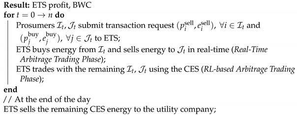
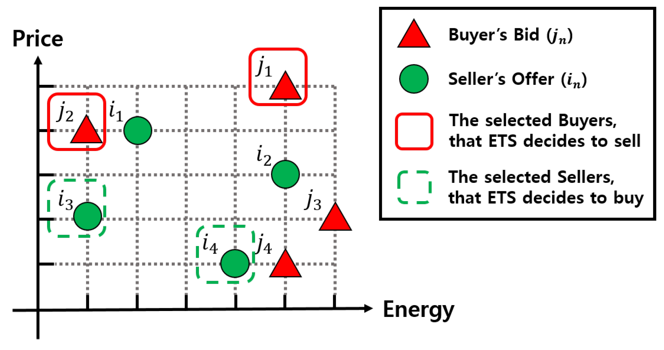
4.1. Real-Time Arbitrage Trading Phase

In the real-time arbitrage trading phase, the ETS selects prosumers to trade energy. The selected sellers directly send energy to the selected buyers; thus, CES is not used in the real-time arbitrage trading phase. Figure 2 shows an example with four buyers and four sellers in the market at a certain time t. The ETS selects to trade with sellers $i_3$ and $i_4$ who have submitted a lower offer price compared to other sellers. The energy bought from $i_3$ and $i_4$ is sold to buyers $j_1$ and $j_2$, who have submitted the higher bid price compared to other buyers. The real-time arbitrage trading phase can be formulated by an optimization problem as follows:

$$\begin{array}{cc}\hfill & \underset{{\mathbf{X}}^{\mathrm{buy}},{\mathbf{X}}^{\mathrm{sell}}}{max}\sum _{j\in {\mathcal{J}}_t}{p}_j^{\mathrm{buy}}{x}_j^{\mathrm{buy}}-\sum _{i\in {\mathcal{I}}_t}{p}_i^{\mathrm{sell}}{x}_i^{\mathrm{sell}}\hfill \\ \hfill & \mathrm{subject}\mathrm{to}\sum _{j\in {\mathcal{J}}_t}{x}_j^{\mathrm{buy}}-\sum _{i\in {\mathcal{I}}_t}{x}_i^{\mathrm{sell}}=0\hfill \\ \hfill & 0\le x_i^{\mathrm{sell}}\le e_i^{\mathrm{sell}},\forall i\in {\mathcal{I}}_t\hfill \\ \hfill & 0\le x_j^{\mathrm{buy}}\le e_j^{\mathrm{buy}},\forall j\in {\mathcal{J}}_t,\hfill \end{array}$$

(3)

where $x_i^{\mathrm{sell}}\in {\mathbf{X}}^{\mathrm{sell}}$ and $x_j^{\mathrm{buy}}\in {\mathbf{X}}^{\mathrm{buy}}$ are the total amounts of energy that would be traded for the ith seller and jth buyer. The first constraint shows that all energy bought from the sellers is sold to the buyers. The last two constraint shows that $x_i^{\mathrm{sell}}$ and $x_j^{\mathrm{buy}}$ should be lower than seller ith offer energy and buyer jth bid energy, respectively.

After the real-time arbitrage trading phase, the prosumers who were not selected by the ETS remain in the market. The remaining prosumers in the market can be seen as prosumers who have failed to submit a proper price to trade with ETS. A formal middleman will stop trading in this phase because the energy cannot be sold with profit in real-time. There is an option of storing the energy in a battery to sell at a higher price, but the BWC cost should be considered while using a battery. Herein, ETS tries to trade with the remaining prosumers using CES. The details of how ETS trades with these remaining prosumers are described in the following subsection.

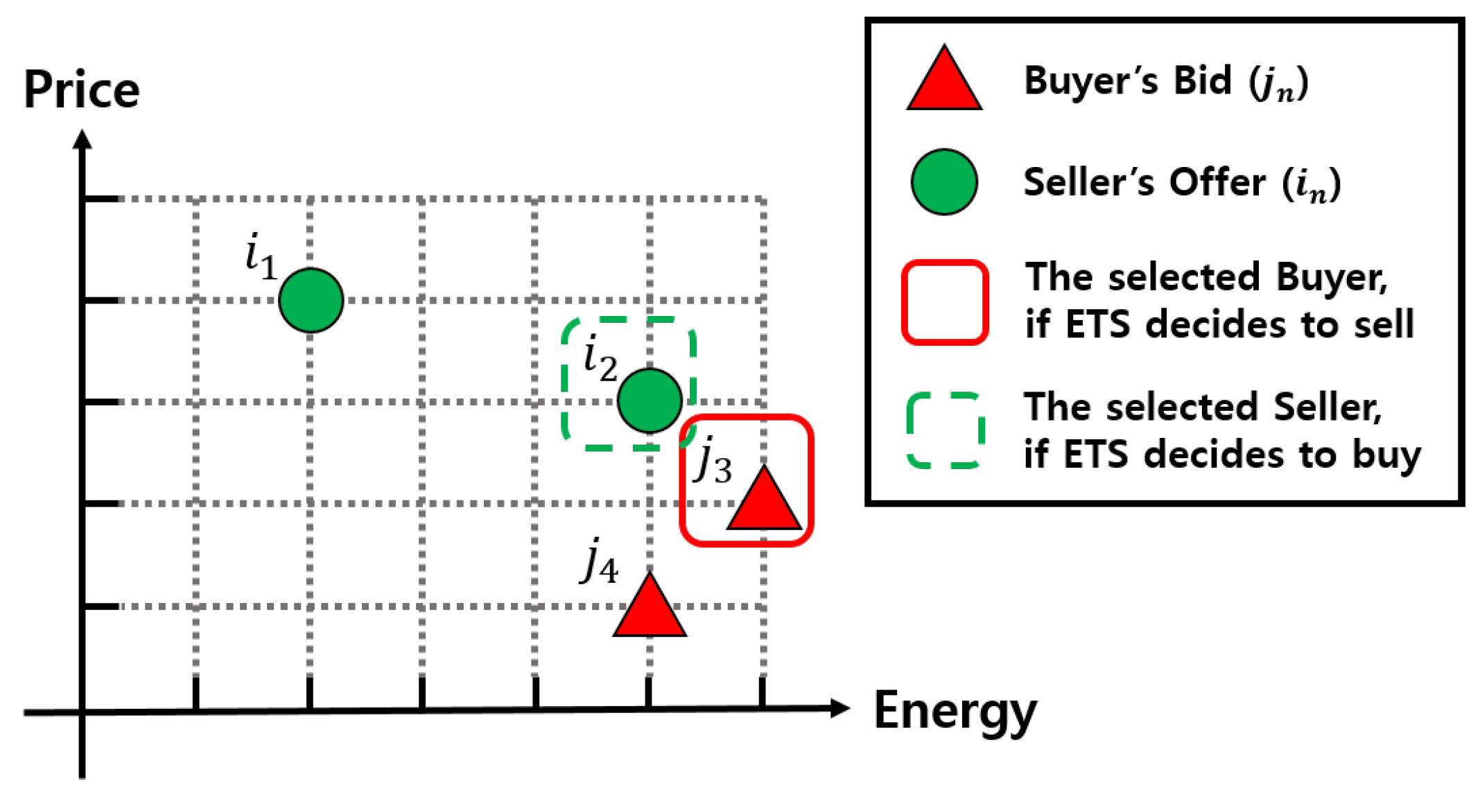
4.2. RL-Based Arbitrage Trading with CES Phase

In RL-based arbitrage trading with the CES phase, the ETS decides whether to trade energy with a prosumer who failed to trade in the real-time arbitrage trading phase. The objective of RL-based arbitrage trading with the CES phase is to maximize the ETS profit using CES, thereby maximizing the amount of energy to be traded between prosumers. If ETS decides to buy energy from a seller, the seller’s energy is stored in CES. If ETS decides to sell energy to a buyer, the CES energy is sent to that buyer.

After real-time arbitrage trading phase (Figure 2) is completed, the market would be as shown in Figure 3, which presents the prosumers who failed to trade with the ETS. The ETS decides whether to buy energy from a seller, sell energy to a buyer, or do nothing. If the ETS decides to buy energy, the ETS buys energy from $i_2$, who submitted the lowest offer price, and if the ETS decides to sell energy, the ETS sells energy to $j_3$, who submitted the highest bid price. The action of ETS at time t is defined as $a_t$, and the action space $\mathcal{A}$ is defined as follows:

$$\mathcal{A}=\{a_{\mathrm{charge}},a_{\mathrm{discharge}},a_{\mathrm{idle}}\},$$

(4)

where $a_{\mathrm{charge}}$ is the action of buying energy from a seller and storing it in CES, $a_{\mathrm{discharge}}$ is the action of selling the energy stored in CES to a buyer, and $a_{\mathrm{idle}}$ represents the action of doing nothing at time t.

The ETS refers to three state values to decide which action maximizes the profit. These values are $o_t$, $b_t$, and $c_t$, related to the seller’s offer price, buyer’s bid price, and CES state of charge (SOC), respectively. The aforementioned variables are used as a part of the state $s_t$, which is defined as:

$$s_t=(o_t,b_t,c_t)\in \mathcal{S},$$

(5)

where S denotes the state space. The first state variable $o_t$ is the converted value of $p_t^{\mathrm{charge}}$, representing the relative price of the seller. The value of $p_t^{\mathrm{charge}}$ is calculated as follows:

$$p_t^{\mathrm{charge}}=\frac{\underset{i\in {\mathcal{I}}_t}{min}\left(p_i^{\mathrm{sell}}\right)-p^{\mathrm{feed}-\mathrm{in}}}{p^{\mathrm{rate}}-p^{\mathrm{feed}-\mathrm{in}}-\eta },$$

(6)

where $p_t^{\mathrm{charge}}$ is set to have a value in the range of $0\le p_t^{\mathrm{charge}}\le 1$. The value of $p_t^{\mathrm{charge}}$ is replaced by $o_t$, which is an integer in the range of $0\le o_t\le 9$. The value of $p_t^{\mathrm{charge}}$ is converted to $o_t$ as follows:

$$o_t=\left\{\begin{array}{cc}0,\hfill & \mathrm{if}\mathrm{there}\mathrm{are}\mathrm{no}\mathrm{sellers}\mathrm{in}\mathrm{RL}-\mathrm{based}\mathrm{arbitrage}\mathrm{trading}\mathrm{phase}\hfill \\ n,\hfill & \mathrm{if}0.11\times (n-1)\le p_t^{\mathrm{charge}}<0.11\times n,\mathrm{for}1\le n\le 8,n\in \mathbb{N}\hfill \\ 9,\hfill & \mathrm{otherwise},\hfill \end{array}\right.$$

(7)

where n is a natural number in the range of $1\le n\le 8$.

The second state variable $b_t$ is calculated through the same process as the first state variable $o_t$. The value of $b_t$ is the converted value of the relative price of the buyer. The value of $p_t^{\mathrm{discharge}}$ is calculated as follows:

$$p_t^{\mathrm{discharge}}=\frac{\underset{j\in {\mathcal{J}}_t}{max}\left(p_j^{\mathrm{buy}}\right)-p^{\mathrm{feed}-\mathrm{in}}-\eta }{p^{\mathrm{rate}}-p^{\mathrm{feed}-\mathrm{in}}-\eta },$$

(8)

where $p_t^{\mathrm{discharge}}$ is set to have a value in the range of $0\le p_t^{\mathrm{discharge}}\le 1$. The value of $p_t^{\mathrm{discharge}}$ is replaced by $b_t$, which is an integer in the range of $0\le b_t\le 9$. The value of $p_t^{\mathrm{discharge}}$ is converted to $b_t$ as follows:

$$b_t=\left\{\begin{array}{cc}0,\hfill & \mathrm{if}\mathrm{there}\mathrm{are}\mathrm{no}\mathrm{buyers}\mathrm{in}\mathrm{RL}-\mathrm{based}\mathrm{arbitrage}\mathrm{trading}\mathrm{phase}\hfill \\ n,\hfill & \mathrm{if}0.11\times (n-1)\le p_t^{\mathrm{discharge}}<0.11\times n,\mathrm{for}1\le n\le 8,n\in \mathbb{N}\hfill \\ 9,\hfill & \mathrm{otherwise},\hfill \end{array}\right.$$

(9)

The third state value $c_t$ is a converted value of the CES SOC $d_t^{\mathrm{CES}}$, which is defined as follows:

$$d_t^{\mathrm{CES}}=\frac{e_t^{\mathrm{CES}}}{E^{\mathrm{CES}}},$$

(10)

where $e_t^{\mathrm{CES}}$ is the stored energy in the CES at time t, and $E^{\mathrm{CES}}$ is the capacity of CES. The value of $d_t^{\mathrm{CES}}$ is converted to $c_t$ as follows:

$$c_t=\left\{\begin{array}{cc}0,\hfill & \mathrm{if}\mathrm{the}\mathrm{CES}\mathrm{is}\mathrm{empty}\mathrm{in}\mathrm{RL}-\mathrm{based}\mathrm{arbitrage}\mathrm{trading}\mathrm{phase}\hfill \\ n,\hfill & \mathrm{if}0.11\times (n-1)\le d_t^{\mathrm{CES}}<0.11\times n,\mathrm{for}1\le n\le 8,n\in \mathbb{N}\hfill \\ 9,\hfill & \mathrm{otherwise},\hfill \end{array}\right.$$

(11)

The value of $s_t$ and $a_t$ determines the reward used to learn the RL agent. The reward function $r_t(s_t,a_t)$ is defined as follows:

$$\begin{array}{cc}\hfill r_t(s_t,a_t)& =\left\{\begin{array}{cc}{r}_{\mathrm{buy}},\hfill & \mathrm{if}{a}_t=a_{\mathrm{charge}}\hfill \\ r_{\mathrm{sell}}-p,\hfill & \mathrm{if}{a}_t=a_{\mathrm{discharge}}\hfill \\ 0,\hfill & \mathrm{otherwise},\hfill \end{array}\right.\hfill \end{array}$$

(12)

where $r_{\mathrm{buy}}$ and $r_{\mathrm{sell}}-p$ are the rewards for charge and discharge actions, respectively. The variable p is the penalty for trying to sell energy when there are no buyers. Each reward is defined as follows:

$$\begin{array}{cc}\hfill r_{\mathrm{buy}}& =g_{\mathrm{buy}}(p^{\mathrm{rate}}-\eta -\underset{i\in {\mathcal{I}}_t}{min}\left(p_i^{\mathrm{sell}}\right))-h_{\mathrm{buy}}{d}_t^{\mathrm{CES}},\hfill \\ \hfill r_{\mathrm{sell}}& =g_{\mathrm{sell}}(\underset{j\in {\mathcal{J}}_t}{max}\left(p_j^{\mathrm{buy}}\right)-p_i^{\mathrm{sell}})+h_{\mathrm{sell}}{d}_t^{\mathrm{CES}},\hfill \\ \hfill p& =\left\{\begin{array}{cc}\beta ,\hfill & \mathrm{if}{b}_t=0\hfill \\ 0,\hfill & \mathrm{otherwise},\hfill \end{array}\right.\hfill \end{array}$$

(13)

where $g_{\mathrm{buy}}$ and $g_{\mathrm{sell}}$ are the coefficients to control the effect of the price, and $h_{\mathrm{buy}}$ and $h_{\mathrm{sell}}$ are the coefficients to control the effect of the amount of energy that remains in CES. The value $h_{\mathrm{buy}}{d}_t^{\mathrm{CES}}$ is subtracted to obtain $r_{\mathrm{buy}}$, which makes the RL agent avoid buying energy if there is much energy in CES. In the case of $r_{\mathrm{sell}}$, the value $h_{\mathrm{sell}}{d}_t^{\mathrm{CES}}$ is added to the reward that makes the RL agent sell energy if there is a lot of energy in CES.

The Q-learning algorithm is employed to maximize the amount of energy to be traded between prosumers by finding the optimal policy that maximizes the profit of the arbitrage trade of the ETS [34]. The Q-table is updated as follows:

$$Q^{\mathrm{new}}(s_t,a_t)=(1-\alpha )Q(s_t,a_t)+\alpha r_t(s_t,a_t)+\alpha \gamma \underset{a}{max}Q(s_{t+1},a),$$

(14)

where $\alpha$ is the learning rate, and $\gamma$ is the discount factor.

5. Numerical Simulation

Section 5.1 describes the transaction data of prosumers and the learning parameters used for the simulation. Section 5.2 shows the simulation results of CES’s economic benefits and the average profit of the proposed algorithm. In the last section, Section 5.3, we compare the profit of the proposed algorithm in the RL-based arbitrage trading phase to other kinds of trading strategies.

5.1. Simulation Setting

The setting used for the simulation is shown in

Table 1. Values and units of each notation.

Notations	Descriptions	Values	Units
n	Number of time step	72	-
T	Interval between time steps	$\frac{24\mathrm{h}}{n}$	-
$\left|I\right|$	Number of sellers	50	-
$\left|J\right|$	Number of buyers	50	-
$t_i^{\mathrm{sell}}$	Market entry time of seller i	$\mathcal{N}(\mu =39,{\sigma }^2={12}^2)$	T
$t_j^{\mathrm{buy}}$	Market entry time of buyer j	$\mathcal{N}(\mu =54,{\sigma }^2={12}^2)$	T
$w_i^{\mathrm{sell}}$	Waiting time of seller i	w	T
$w_j^{\mathrm{buy}}$	Waiting time of buyer j	w	T
w	Waiting time of prosumers	0 ~  3	T
$p_i^{\mathrm{sell}}$	Offer price of seller i	$\mathcal{U}(a=0.08,b=0.38)$	$
$p_j^{\mathrm{buy}}$	Bid price of buyer j	$\mathcal{U}(a=0.08,b=0.38)$	$
$e_i^{\mathrm{sell}}$	Offer energy of seller i	$\mathcal{U}(a=20,b=40)$	kWh
$e_j^{\mathrm{buy}}$	Bid energy of buyer j	$\mathcal{U}(a=20,b=40)$	kWh
$\eta$	Price regulation of the ETS	0	$
$E^{\mathrm{CES}}$	Battery capacity	100 ~–800	kWh
$\mu$	Battery efficiency	0.95	-
${\mu }^2$	Battery round trip efficiency	0.9025	-
$\alpha$	Learning rate	0.1	-
$\gamma$	Discount factor	0.1	-
$ϵ$	Epsilon-greedy parameter	0.1	-
$g_{\mathrm{buy}}$	Weight coefficient	5	-
$g_{\mathrm{sell}}$	Weight coefficient	2.5	-
$h_{\mathrm{buy}}$	Weight coefficient	2	-
$h_{\mathrm{sell}}$	Weight coefficient	2	-

. We divided each day into 72 time steps, allowing 20-min intervals for an event to occur. We assumed that 50 buyers and 50 sellers enter the market once per day. The transaction data of prosumers are generated for each day with the distribution shown in Table 1. Many sellers enter the market around noon when the amount of PV generation is expected to be high, and many buyers enter the market in the afternoon when the amount of energy use is expected to be high. The prosumers’ waiting time is fixed to w, which is a constant value ranging from 0 to 3. The average feed-in tariff and service rate in Germany is used as the boundary value of $p_i^{\mathrm{sell}}$ and $p_j^{\mathrm{buy}}$ [35,36]. In this study, the ETS does not regulate the prosumers’ price, so $\eta$ is set to 0. We assume that CES uses a lithium-ion battery pack, which costs $137 per kWh [37]. The battery efficiency is 0.95, which elicits about 90% of round trip efficiency. The capacity of the CES is 400 kWh, except for the simulation in Section 5.3 that shows the ETS profit for the CES capacity ranging from 100 to 800 kWh. The Q-learning parameters, including learning rate $\alpha$, discount factor $\gamma$, and $ϵ$ greedy parameter, are set to 0.1.

5.2. Simulation Results

In order to validate the economic benefits of using CES, we compared the total profit resulting from RL-based arbitrage trading to the CES phase with BWC. The total profit includes the ETS profit and the prosumers’ profit from trading with the ETS instead of the utility. The total profit obtained by the proposed trading algorithm is defined as follows:

$$\mathrm{Total}\mathrm{Profit}=\mathrm{ETS}\mathrm{Profit}+\mathrm{Sellers}\mathrm{Profit}+\mathrm{Buyers}\mathrm{Profit},$$

(15)

$$\mathrm{Sellers}\mathrm{Profit}=\sum _{i\in \mathcal{I}}(p_i^{\mathrm{sell}}-p^{\mathrm{feed}-\mathrm{in}})x_i^{\mathrm{sell}},$$

(16)

$$\mathrm{Buyers}\mathrm{Profit}=\sum _{j\in \mathcal{J}}(p^{\mathrm{rate}}-p_j^{\mathrm{buy}})x_j^{\mathrm{buy}},$$

(17)

where $p_i^{\mathrm{sell}}-p^{\mathrm{feed}-\mathrm{in}}$ and $p^{\mathrm{rate}}-p_j^{\mathrm{buy}}$ indicate the price advantage of prosumer i and j can obtain by trading with ETS instead of the utility.

BWC when the stored energy in the battery changes from $e_{t+1}^{\mathrm{CES}}$ to $e_t^{\mathrm{CES}}$ can be defined as follows:

$$\mathrm{BWC}=|e_{t+1}^{\mathrm{CES}}-e_t^{\mathrm{CES}}|\times \mathrm{AWC}\left(D\right),$$

(18)

where $\mathrm{AWC}\left(D\right)$ is the average wear-cost per unit of energy transfer, and the inner variable D indicates the battery depth of discharge (DOD). The AWC per kWh is formulated using an existing BWC model in [27] as follows:

$$\begin{array}{cc}\hfill \mathrm{AWC}\left(D\right)& =\frac{\mathrm{Battery}\mathrm{Price}}{\mathrm{Total}\mathrm{Transferable}\mathrm{Energy}\mathrm{During}\mathrm{the}\mathrm{Life}\mathrm{Cycle}}\hfill \\ \hfill & =\frac{\mathrm{Battery}\mathrm{Price}}{\mathrm{ACC}\left(D\right)\times 2\times D\times E^{\mathrm{CES}}\times {\mu }^2},\hfill \end{array}$$

(19)

where $\mu$ is the battery efficiency, and ${\mu }^2$ indicates the round-trip efficiency of the battery. $\mathrm{ACC}\left(D\right)$ is the average cycle count of a typical lithium-ion battery, which is defined as follows:

$$\mathrm{ACC}\left(D\right)=\frac{a}{D^b},$$

(20)

where a and b are battery-dependent parameters that can be acquired experimentally. However, batteries that are made with the same material do not have the exact same battery wear characteristics and thus need to be checked by experiments. The most typical specifications are given by the battery manufacturers with respect to the DOD. Herein, we applied the values of a typical lithium-ion battery, which are $a=694$ and $b=0.795$ [27]. A lithium-ion battery pack cost $137/kWh in 2020 [37]. We assume the other variable as $D=1$ and $\mu =0.95$; thus, $\mathrm{AWC}\left(1\right)=\$0.1093/\mathrm{kWh}$.

Figure 4 presents the total profit and BWC resulting from the RL-based arbitrage trading phase. The total profit is about $105.34 per day, and BWC is about $77.89 per day. This result reveals that the proposed algorithm using CES yields a profit of $27.45 per day in the proposed LEM. If we consider social benefits, such as the decrease in grid consumption, we expect far more profits than the result.

Figure 5 shows the daily profit of ETS. The ETS Profit with CES graph represents the ETS profit using the proposed energy trade management algorithm. The ETS Profit without CES graph represents the ETS profit using the proposed energy trade management algorithm without RL-based arbitrage trading with the CES phase but only with real-time arbitrage trading phase since it assumes that the ETS has no CES. The daily average of the ETS profit is $69.58 and $36.22, respectively. The ETS can earn about $33.36 more using the CES.

Figure 6 and Figure 7 show the average profit per day for the proposed algorithm and the CES first algorithm. The CES first algorithm is an energy trade management algorithm where the RL-based arbitrage trading phase starts before the real-time arbitrage trading phase. The CES first algorithm uses CES to trade with a prosumer who submitted the highest bid price or lowest offer price that can be traded with a high probability in the RL-based arbitrage trading phase. This results in a lower profit of the CES first algorithm compared to that of the proposed algorithm. There is a slight increase in the ETS profit if prosumers wait for a certain time w to trade in the LEM, but there is no big difference in the total profit. In Figure 6, the proposed algorithm shows an ETS profit of $69.58 and a total profit of $105.34, and the CES first algorithm shows an ETS profit of $56.08 and a total profit of $89.37. In Figure 7, the proposed algorithm shows an ETS profit of $71.99 and a total profit of $105.29, and the CES first algorithm shows an ETS profit of $67.10 and a total profit of $91.39.

5.3. Simulation Analysis

In order to verify the performance of RL-based arbitrage trading in the proposed algorithm, we compared the trading profit with that of three other trading strategies. The first trading strategy is the previous action maintain (PAM), which repeats the action chosen at the previous time step. PAM starts with buying energy until the CES reaches its capacity, and after reaching the capacity, PAM then repeats selling energy. The second strategy is called random action as it chooses actions in a random order. The last trading strategy is named optimal, which gives the maximum profit with the perfect forecast of the whole day’s transaction.

Figure 8 and Figure 9 show the CES discharge rate and ETS profit with respect to the CES capacity. The 100-day trading result is used to calculate the daily average of CES discharge rate and ETS profit. The RL-based arbitrage trading in the proposed algorithm reveals a high discharge rate, 0.97 on average, and the profit increases slightly as the CES capacity increases. PAM also shows a high discharge rate of 0.98 when the CES capacity is 400 kWh. However, there is a big difference in the ETS profit. PAM shows a profit of $9.02 per day when the CES capacity is 400 kWh, whereas RL-based arbitrage trading in the proposed algorithm shows a profit of $33.36 per day for the same CES capacity.

Figure 10, Figure 11, Figure 12 and Figure 13 show the details of 100-day trading when the CES capacity is 400 kWh. Figure 10 shows the daily profit of the ETS for each trading strategy. The optimal strategy shows a profit of $55.5 per day, resulting in a high selling price of energy with no surplus energy in the CES. In the case of other trading strategies, we assume that the remaining energy in the CES after a day is sold to the utility company. This prevents the CES from being overloaded by energy having a low possibility of being sold to another prosumer.

Figure 11 and Figure 12 show the pattern of the daily use of CES. Since CES is used for prosumers who failed to trade in the real-time arbitrage trading phase, the daily use graph of the CES is irregular. PAM shows a typical CES use pattern compared to that of other algorithms as it does not consider the price of a prosumer but only the SOC of CES. RL-based arbitrage trading in the proposed algorithm shows an irregular CES use pattern, but the charge and discharge graphs are similar, indicating the high selling rate of the proposed algorithm.

Figure 13 shows the daily discharge rate for each algorithm. The daily discharge rate shows the selling rate of arbitrage trading. PAM also shows a high discharge rate compared to the RL-based arbitrage trading of the proposed algorithm. However, as we have seen above, PAM was not able to sell its energy at a time when the prosumer price is high.

In addition, we have analyzed the performance of the RL-based trading algorithm with different sizes of $s_t$. Figure 14 shows the daily profit of the ETS in RL-based arbitrage trading phase when the CES capacity is 400 kWh. Increasing the size $s_t$ from 5 × 5 × 5 to 10 × 10 × 10 shows an increase in profit of about $3.01, but increasing the size from 10 × 10 × 10 to 15 × 15 × 15 shows a small decrease of about $1.18 in profit. According to the simulation result, decreasing the size of $s_t$ results in a smaller profit, but increasing the size of $s_t$ did not result in a bigger profit.

6. Conclusions and Discussion

In this study, an energy-trade management algorithm is proposed for managing the trade of prosumers using CES. We designed and modeled a LEM that manages the trade of prosumers who are not controlled by a central operator and act competitively with other prosumers. The CES is managed by an RL-based algorithm and used for prosumers who fail to trade in the real-time trading phase. Numerical simulations show that there are more economic benefits if the CES is limited to prosumers who fail to trade in the real-time trading phase. The main parameters considered in the numerical simulations are the ETS profit from trading with prosumers, the prosumers profit from trading with the ETS instead of the utility, and BWC. Numerical simulations show that the total trading profit by using the CES is higher than the BWC. The primary results of the numerical simulations are as follows:

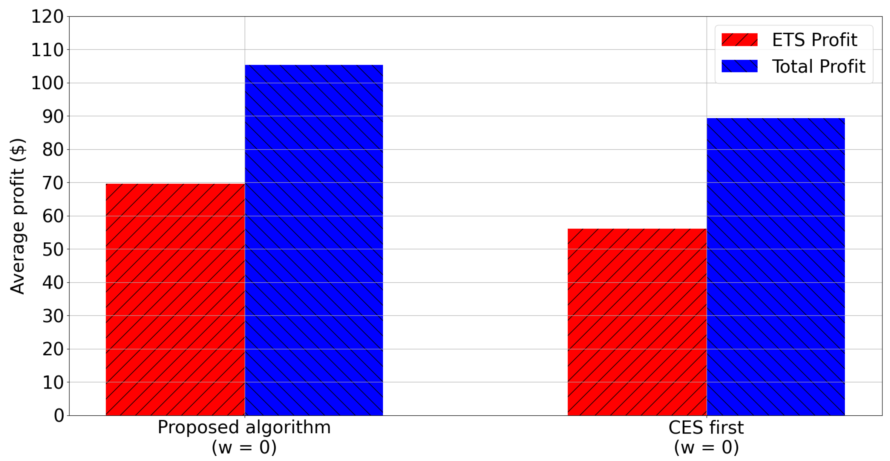
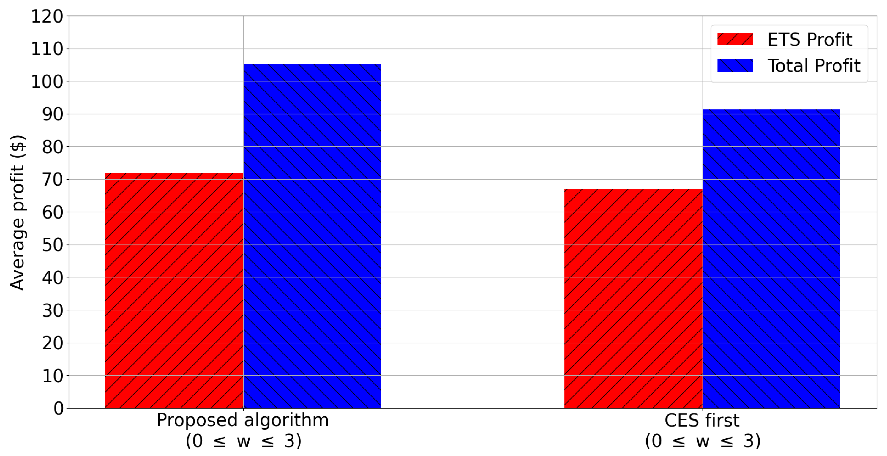
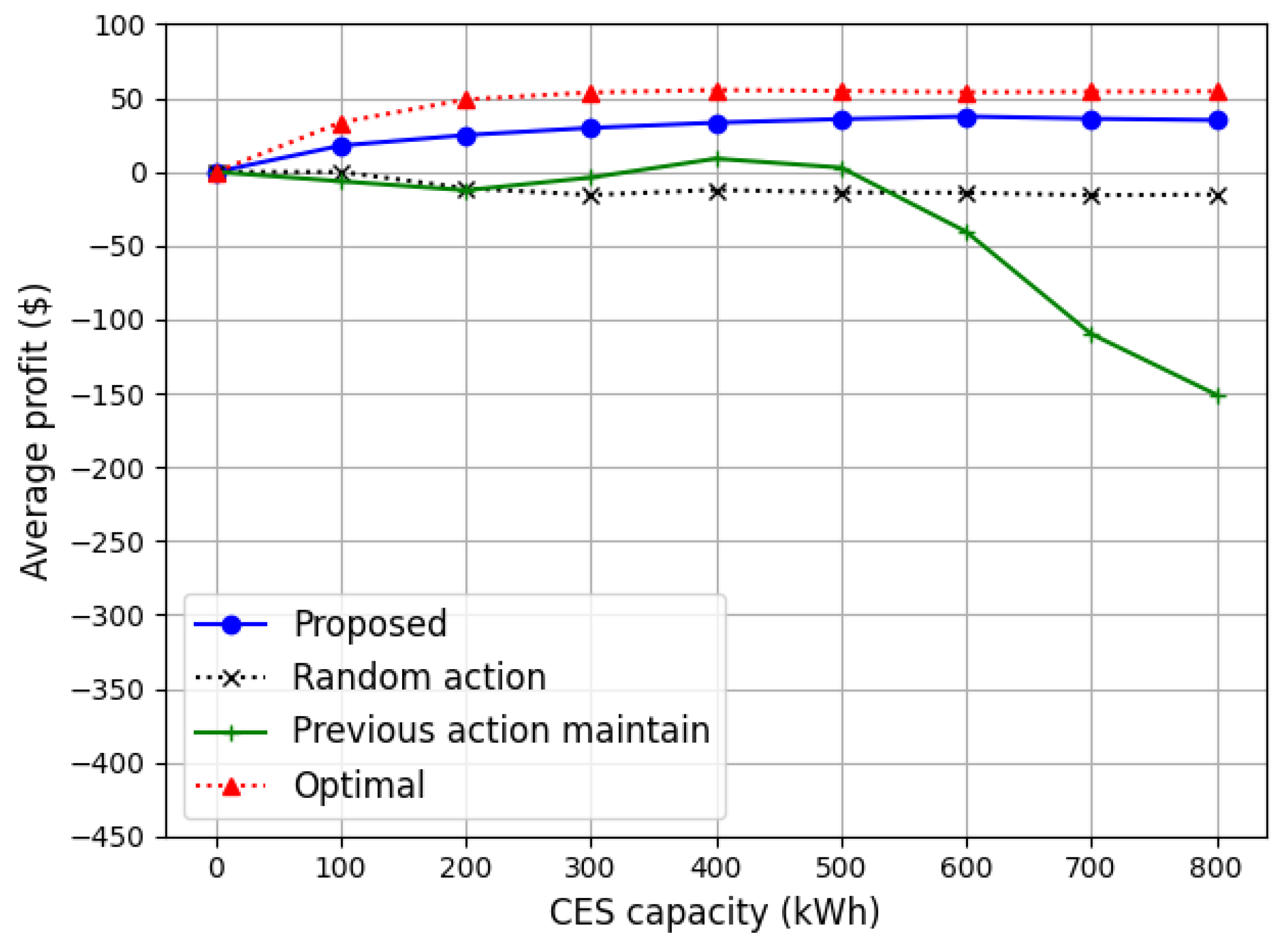
• The total profit of the proposed energy management algorithm is $105.34 per day. If CES is used in the real-time trading phase, the total profit decreases to $89.37 per day.
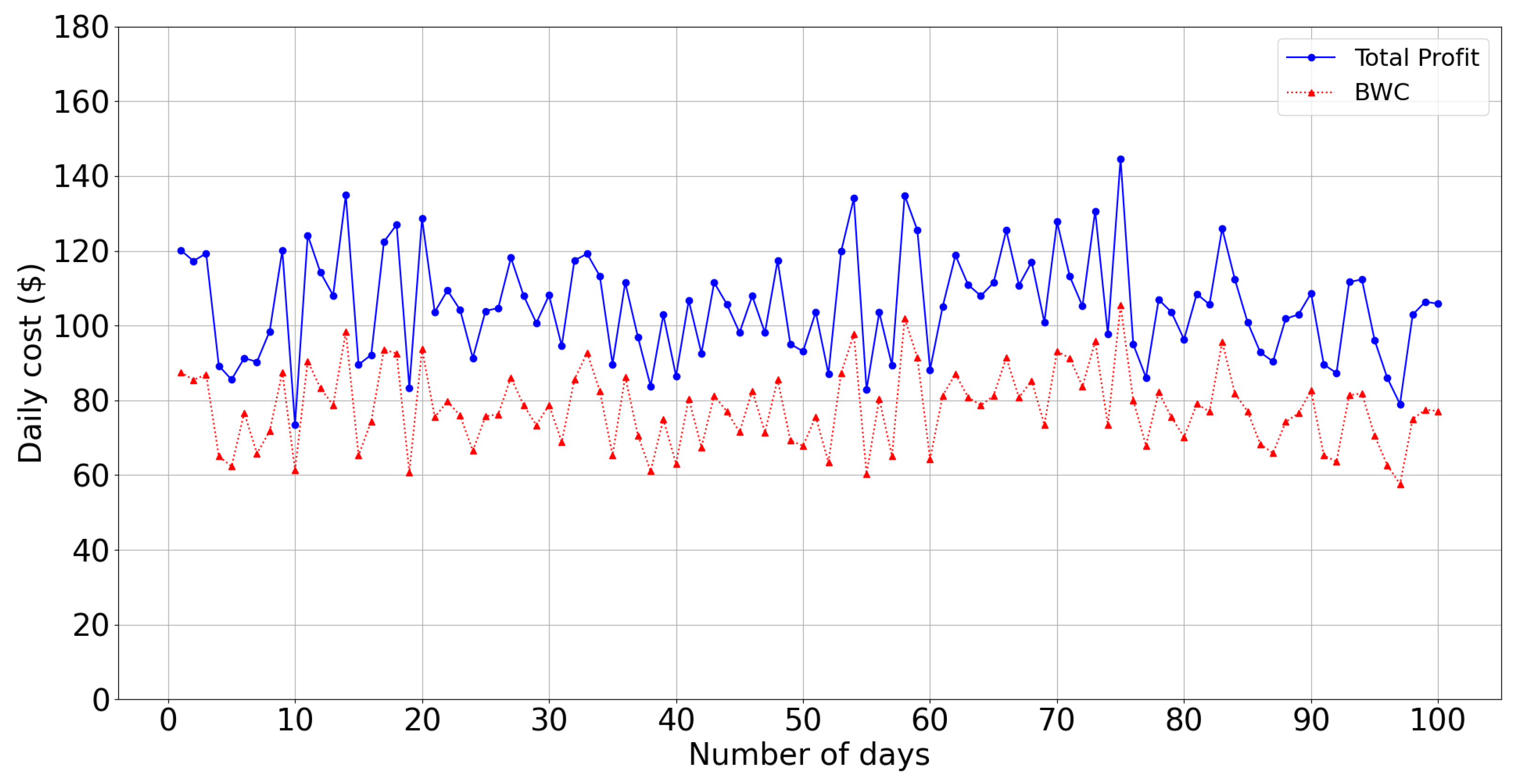
• The BWC of the proposed energy management algorithm is about $77.89 per day. This result reveals that the proposed algorithm using CES yields a profit of $27.45 per day in the proposed LEM.

There are two limitations to this study, which we shall address in our future studies. First, instead of generating the simulation data with specific mean and deviations, we hope to analyze and apply real-world energy transaction data of prosumers. Second, since the Q-learning algorithm has problems using continuous values for the state and action, we can adopt a novel RL algorithm to trade more efficiently in the proposed LEM.

References

1. Energy and the Environment Explained: Where Greenhouse Gases Come From. Available online: https://www.eia.gov/energyexplained/energy-and-the-environment/where-greenhouse-gases-come-from.php (accessed on 2 January 2021).
2. Sources of Greenhouse Gas Emissions. Available online: https://www.epa.gov/ghgemissions/sources-greenhouse-gas-emissions (accessed on 4 January 2021).
3. Global Trends in Renewable Energy Investment. 2019. Available online: https://wedocs.unep.org (accessed on 6 January 2021).
4. Parag, Y.; Sovacool, B.K. Electricity market design for the prosumer era. Nat. Energy 2016, 1, 1–6. [Google Scholar] [CrossRef]
5. Brooklyn Microgrid|Community Powered Energy. Available online: https://www.brooklyn.energy/ (accessed on 8 January 2021).
6. Roberts, M.B.; Bruce, A.; MacGill, I. Impact of shared battery energy storage systems on photovoltaic self-consumption and electricity bills in apartment buildings. Appl. Energy 2019, 245, 78–95. [Google Scholar] [CrossRef]
7. Mediwaththe, C.P.; Stephens, E.R.; Smith, D.B.; Mahanti, A. Competitive energy trading framework for demand-side management in neighborhood area networks. IEEE Trans. Smart Grid 2017, 9, 4313–4322. [Google Scholar] [CrossRef] [Green Version]
8. Albadi, M.H.; El-Saadany, E.F. A summary of demand response in electricity markets. Electric Power Syst. Res. 2008, 78, 1989–1996. [Google Scholar] [CrossRef]
9. Chen, S.; Liu, C.C. From demand response to transactive energy: State of the art. J. Mod. Power Syst. Clean Energy 2017, 5, 10–19. [Google Scholar] [CrossRef] [Green Version]
10. Daneshvar, M.; Mohammadi-Ivatloo, B.; Asadi, S.; Anvari-Moghaddam, A.; Rasouli, M.; Abapour, M.; Gharehpetian, G.B. Chance-constrained models for transactive energy management of interconnected microgrid clusters. J. Clean. Prod. 2020, 271, 122177. [Google Scholar] [CrossRef]
11. Nizami, M.S.H.; Hossain, J.; Fernandez, E. Multi-agent based transactive energy management systems for residential buildings with distributed energy resources. IEEE Trans. Ind. Inform. 2019, 16, 1836–1847. [Google Scholar] [CrossRef]
12. Koltsaklis, N.; Panapakidis, I.P.; Pozo, D.; Christoforidis, G.C. A Prosumer Model Based on Smart Home Energy Management and Forecasting Techniques. Energies 2021, 14, 1724. [Google Scholar] [CrossRef]
13. Celik, B.; Roche, R.; Bouquain, D.; Miraoui, A. Decentralized neighborhood energy management with coordinated smart home energy sharing. IEEE Trans. Smart Grid 2017, 9, 6387–6397. [Google Scholar] [CrossRef] [Green Version]
14. Akter, M.N.; Mahmud, M.A.; Haque, M.E.; Oo, A.M. An optimal distributed energy management scheme for solving transactive energy sharing problems in residential microgrids. Appl. Energy 2020, 270, 115133. [Google Scholar] [CrossRef]
15. Akter, M.N.; Mahmud, M.A.; Oo, A.M. A hierarchical transactive energy management system for microgrids. In Proceedings of the 2016 IEEE Power and Energy Society General Meeting (PESGM), Boston, MA, USA, 17–21 July 2016; pp. 1–5. [Google Scholar]
16. Zhang, C.; Wu, J.; Zhou, Y.; Cheng, M.; Long, C. Peer-to-Peer energy trading in a Microgrid. Appl. Energy 2018, 220, 1–12. [Google Scholar] [CrossRef]
17. Chen, T.; Su, W. Local energy trading behavior modeling with deep reinforcement learning. IEEE Access 2018, 6, 62806–62814. [Google Scholar] [CrossRef]
18. Chen, T.; Su, W. Indirect customer-to-customer energy trading with reinforcement learning. IEEE Trans. Smart Grid 2018, 10, 4338–4348. [Google Scholar] [CrossRef]
19. Long, C.; Zhou, Y.; Wu, J. A game theoretic approach for peer to peer energy trading. Energy Procedia 2019, 159, 454–459. [Google Scholar] [CrossRef]
20. Jing, R.; Xie, M.N.; Wang, F.X.; Chen, L.X. Fair P2P energy trading between residential and commercial multi-energy systems enabling integrated demand-side management. Appl. Energy 2020, 262, 114551. [Google Scholar] [CrossRef]
21. Bose, S.; Kremers, E.; Mengelkamp, E.M.; Eberbach, J.; Weinhardt, C. Reinforcement learning in local energy markets. Energy Inform. 2021, 4, 1–21. [Google Scholar] [CrossRef]
22. Kim, J.G.; Lee, B. Automatic P2P Energy Trading Model Based on Reinforcement Learning Using Long Short-Term Delayed Reward. Energies 2020, 13, 5359. [Google Scholar] [CrossRef]
23. Guerrero, J.; Chapman, A.C.; Verbič, G. Decentralized P2P energy trading under network constraints in a low-voltage network. IEEE Trans. Smart Grid 2018, 10, 5163–5173. [Google Scholar] [CrossRef] [Green Version]
24. Thakur, S.; Hayes, B.P.; Breslin, J.G. Distributed double auction for peer to peer energy trade using blockchains. In Proceedings of the 2018 5th International Symposium on Environment-Friendly Energies and Applications (EFEA) IEEE, Rome, Italy, 24–26 September 2018; pp. 1–8. [Google Scholar]
25. Umer, K.; Huang, Q.; Khorasany, M.; Afzal, M.; Amin, W. A novel communication efficient peer-to-peer energy trading scheme for enhanced privacy in microgrids. Appl. Energy 2021, 296, 117075. [Google Scholar] [CrossRef]
26. Bucciarelli, M.; Paoletti, S.; Vicino, A. Optimal sizing of energy storage systems under uncertain demand and generation. Appl. Energy 2018, 225, 611–621. [Google Scholar] [CrossRef]
27. Han, S.; Han, S.; Aki, H. A practical battery wear model for electric vehicle charging applications. Appl. Energy 2014, 113, 1100–1108. [Google Scholar] [CrossRef]
28. Nykvist, B.; Nilsson, M. Rapidly falling costs of battery packs for electric vehicles. Nat. Clim. Chang. 2015, 5, 329–332. [Google Scholar] [CrossRef]
29. Koirala, B.P.; van Oost, E.; van der Windt, H. Community energy storage: A responsible innovation towards a sustainable energy system? Appl. Energy 2018, 231, 570–585. [Google Scholar] [CrossRef]
30. Anvari-Moghaddam, A.; Rahimi-Kian, A.; Mirian, M.S.; Guerrero, J.M. A multi-agent based energy management solution for integrated buildings and microgrid system. Appl. Energy 2017, 203, 41–56. [Google Scholar] [CrossRef] [Green Version]
31. Lüth, A.; Zepter, J.M.; del Granado, P.C.; Egging, R. Local electricity market designs for peer-to-peer trading: The role of battery flexibility. Appl. Energy 2018, 229, 1233–1243. [Google Scholar] [CrossRef] [Green Version]
32. Double Auction. Available online: https://en.wikipedia.org/wiki/Double_auction (accessed on 26 January 2021).
33. Feed-in Tariff. Available online: https://en.wikipedia.org/wiki/Feed-in_tariff (accessed on 29 January 2021).
34. Q-Learning. Available online: https://en.wikipedia.org/wiki/Q-learning (accessed on 9 January 2021).
35. What German Households Pay for Power. Available online: https://www.cleanenergywire.org/factsheets/what-german-households-pay-power (accessed on 19 January 2021).
36. Germany Installed 700 MW of PV in First Two Months of 2020. Available online: https://www.pv-magazine.com/2020/04/01/germany-installed-700-mw-of-pv-in-first-two-months-of-2020/ (accessed on 19 January 2021).
37. Battery Pack Prices Cited Below $100/kWh for the First Time in 2020, While Market Average Sits at $137/kWh. Available online: https://about.bnef.com/blog/battery-pack-prices-cited-below-100-kwh-for-the-first-time-in-2020-while-market-average-sits-at-137-kwh/ (accessed on 19 January 2021).
Figure 1. LEM design with a centralized CES.
Energies 14 04131 g001
Figure 2. An example of real-time arbitrage trading.
Energies 14 04131 g002
Figure 3. An example of RL-based arbitrage trading with CES.
Energies 14 04131 g003
Figure 4. The rotal profit and BWC by using the CES.
Energies 14 04131 g004
Figure 5. The daily profit of ETS with and without CES.
Energies 14 04131 g005
Figure 6. The average profit per day of two algorithms with w = 0 .
Energies 14 04131 g006
Figure 7. The average profit per day of two algorithms with 0 w 3 .
Energies 14 04131 g007
Figure 8. The average discharge rate with respect to CES capacity.
Energies 14 04131 g008
Figure 9. The average ETS profit with respect to CES capacity.
Energies 14 04131 g009
Figure 10. Daily profit of ETS for each policy.
Energies 14 04131 g010
Figure 11. The daily amount of energy charged to CES.
Energies 14 04131 g011
Figure 12. The daily amount of energy discharged from CES.
Energies 14 04131 g012
Figure 13. The daily discharge rate of CES for each policy.
Energies 14 04131 g013
Figure 14. The average ETS profit for different sizes of s t .
Energies 14 04131 g014