Mathematical Modelling of a System for Solar PV Efficiency Improvement Using Compressed Air for Panel Cleaning and Cooling

Abstract

The efficiency of solar photovoltaic (PV) panels is greatly reduced by panel soiling and high temperatures. A mechanism for eliminating both of these sources of inefficiencies is presented by integrating solar PV generation with a compressed air system. High-pressure air can be stored and used to blow over the surface of PV panels, removing present dust and cooling the panels, increasing output power. A full-system mathematical model of the proposed system is presented, comprised of compressed air generation and storage, panel temperature, panel cleaning, and PV power generation. Simulation results indicate the benefit of employing compressed air for cleaning and cooling solar PV panels. For a fixed volume of compressed air, it is advantageous to blow air over the panels early in the day if the panel is soiled or when solar radiation is most abundant with the highest achievable flow rate if the panel is clean. These strategies have been shown to achieve the greatest energy captures for a single PV panel. When comparing the energy for air compression to the energy gain from cleaning a single PV over a two-week period, an energy ROI of 23.8 is determined. The system has the potential to eliminate the requirement for additional manual cleaning of solar PV panels.

1. Introduction

Solar photovoltaics (PV) are a technology for renewable electricity generation that are becoming increasingly cost-effective [1]. Research output in the field of solar PV is increasing exponentially, driven by the green agenda in a number of countries [2]. As such, it is expected that PV generation will become one of the dominant methods of power generation in the coming decades as nations aim to decarbonise their power sectors [3]. However, the overall efficiency of PV generation is significantly reduced by the effects of panel soiling [4]. When dust or similar particles become attached to the surface of a PV panel, light is blocked from reaching the current producing photodiodes and overall power production falls. It is reported that in some locales, panel soiling is responsible for a 15–17% drop in power output across a one-month period [5]. Similar studies indicate that for some locations, losses exceeding a 50% reduction in power output can be observed when left untreated for a year [6]. The deposition of dust has also been shown to cause permanent degradation of the surface properties of panels and limit the total service lifetime [7] because of uneven temperature distributions arising from non-uniform soiling [8].

Additionally, PV generation is greatly influenced by the temperature of the panel, with high temperatures resulting in a decrease in power output. An increase in temperature corresponds to a decrease in the semiconductor band gap energy of the cells; thus, a smaller amount of energy is produced for a constant level of irradiance at a higher panel temperature [9]. Large and repeated fluctuations in panel temperatures also accelerate panel degradation, as panels experience thermal stress from heating and cooling across a wide temperature range [10] and enhance the effects of other degradation factors (e.g., hydrolysis and photodegradation) [11]. The combined effects of soiling and excessive temperatures are regular, owing to the locations of many large-scale PV installations; locations with an abundant solar resource are often dry, arid environments where soiling and high temperatures commonly coincide.

The efficiency reductions from soiling and heating can be mitigated in a number of ways. Manual cleaning with or without water is an effective method of reducing the presence of dust on the panel surface [12], but this can be expensive and logistically difficult owing to the large scale and remote locations of many PV facilities. Repetitive brushing may also result in damage to the surface of the panel [13]. To mitigate heating effects on PV generation, a number of methods have been proposed [14], employing both active and passive technologies [15], though none of these have become ubiquitous in commercial applications.

This paper proposes the use of compressed air for the cleaning and cooling of PV panels to mitigate the effects of soiling and heating, to improve overall PV generation efficiency. This method has the potential for managing both sources of inefficiency while requiring little maintenance and no water. A novel integrated PV-compressed air mechanism is outlined in this paper, and a full-system mathematical model is derived. A mathematical model incorporating PV generation, a compressed air system, and both the cleaning and cooling mechanisms from high velocity air on PV panels has not previously been reported. The derived model is used to demonstrate the feasibility of the proposed system for improving the efficiency of PV generation by cleaning and cooling the panels. The mechanism is described, and then the individual models of the subcomponents of the charging and discharging processes are presented. Scenarios for the cleaning and cooling of PV panels are simulated, and the possible benefit to PV generation from the implementation of such a system is outlined.

2. Materials and Methods

The proposed PV-compressed air system is comprised of an individual PV panel or an array of panels. A DC motor is coupled with a scroll-type air compressor which feeds a compressed air tank. The stored, high-pressure air is directed to the surface of the panels via a network of pipes. Nozzles fitted to the outlet of the pipes, parallel to the plane of the panel, accelerate the air to blow across the panel surface. This action will result in the removal present dust and will cool the panel via forced convection. The layout of the proposed system is given in Figure 1.

The proposed integrated PV-compressed air system is a robust solution that can be fully automated. This has the potential to reduce expenditure on manual cleaning, which is currently the most utilized method to mitigate soiling losses. Additionally, this system requires no water, which can be scarce and expensive in the arid climates in which many facilities operate. Depending on the size of the compressor and tank used, it is expected that such a system could be applicable to PV installations of all sizes and can be constructed of a modular design. If the compressor is powered by a DC motor, it allows for direct powering from the PV generation, with minimal power conversion necessary. Compared to alternative compressors that could be implemented, such as reciprocating piston or rotary screw compressors, a scroll-type compressor is chosen for implementation in the system because of its high efficiency, robust nature, and minimal maintenance requirement. Therefore, this compressor type is more suited to the application in remote and arid areas [16]. To determine the feasibility and assess the potential of such a system, a comprehensive mathematical model has been derived from independent models of the components and processes.

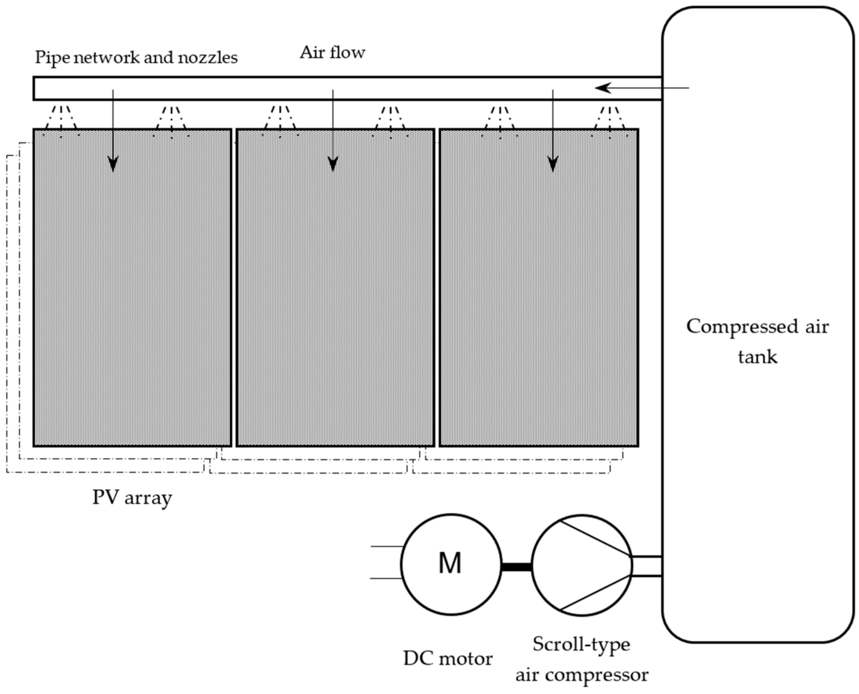
2.1. Full System Mathematical Model

2.1.1. DC Motor

A DC permanent magnet synchronous motor (PMSM) is used to drive the compressor. The rotational acceleration of the rotor, $\ddot{\theta }$, is a function of the rotor inertia, J; the rotor torque, τ; the viscous damping factor, b; the rotor speed, $\dot{\theta }$; and the load torque, τ_L [17]. The rotor is assumed as rigid, and the magnetic field is constant. This is given in Equation (1):

$$\ddot{\theta }=\frac{1}{J}\left(\tau -b\dot{\theta }-{\tau }_L\right)$$

(1)

As the magnetic field is assumed to be constant, the motor torque is directly proportional to the armature current, i, such that

$$\tau =K_{t}i$$

(2)

where K_t is the motor torque constant.

The armature current is a function of the circuit inductance, L_m; the circuit resistance, R_m; the applied voltage, V_DC; and the back electromotive force (emf), e. This is provided in Equation (3):

$$\dot{\dot{i}}=\frac{1}{L_m}\left(-R_{m}i+V_{DC}-e\right)$$

(3)

Similarly, the back emf is proportional to the rotor speed, multiplied by the electromotive force constant, K_e.

$$e=K_e\dot{\theta }$$

(4)

The energy consumed by the operation of the motor is equal to the integral of the power. This is given as

$$E=\int \tau \dot{\theta }$$

(5)

2.1.2. Scroll-Type Air Compressor

A scroll-type compressor is comprised of two meshing scroll blades of identical spiral geometry. One scroll blade is fixed, and the other sits on a shaft capable of orbiting around a fixed path. The meshing blade geometry is presented in Figure 2. As the moving scroll orbits, air is forced through the device as the chamber volumes decrease. The compressor is driven by an electrical motor.

A mathematical model for a scroll-type compressor is derived from a mathematical model of a scroll-type expander [18,19]. In contrast to scroll compressors, which are powered by rotational motion to produce pressurised air, scroll expanders work in reverse, powered by compressed air to produce rotational motion. Thus, the derivations of chamber geometry can be applied for compressors.

The geometry of the moving scroll blade is determined by Equations (6) and (7):

$$x_m=\left({\rho }_0+k\varphi \right)\sin \varphi +k\cos \varphi -k+r\sin \alpha$$

(6)

$$y_m=-\left({\rho }_0+k\varphi \right)\cos \varphi +k\sin \varphi +{\rho }_0-r\cos \alpha$$

(7)

where x_m and y_m denote the x and y coordinates of the moving scroll blade, respectively. The initial radius of curvature of the scroll is given as ρ₀, the opening value of curvature as k, and the angle of rotation as ϕ. The radius of orbit is given as r, and the angle of orbit is given as α.

The coordinates for the enveloping scroll blades can be similarly derived by Equations (8) and (9):

$$x_f=\left({\rho }_0+k\left(\varphi +\pi \right)\right)\sin \left(\varphi +\pi \right)+k\cos \left(\varphi +\pi \right)-k+r\sin \varphi$$

(8)

$$y_f=-\left({\rho }_0+k\left(\varphi +\pi \right)\right)\cos \left(\varphi +\pi \right)+k\sin \left(\varphi +\pi \right)+{\rho }_0-r\cos \varphi$$

(9)

where x_f and y_f are the x and y coordinates of the fixed scroll, respectively.

The volume of the compressor’s inlet chamber is calculated with Equation (10):

$$V_{in}=V_{total}-V_c-V_s$$

(10)

where V_in is the compressor inlet volume, V_total is the total volume occupied by all chambers, V_c is the central chamber volume used as the outlet, and V_s is the volume of the side chambers of the compressors.

The side chamber volume can be calculated using Equation (11):

$$V_s=z\left[\pi r^2+2\pi r\left({\rho }_0+k\alpha \right)\right]$$

(11)

where z is the height of the scroll blade, and the other parameters are the same as Equations (6)–(9). The volume of the central chamber can be calculated with

$$V_c=z\left[\left(kr-\pi k^2\right)\cos \alpha +\left(kr{\rho }_0\pi -r{\rho }_0\right)\sin \alpha +\left(kr\pi +2k{\rho }_0\pi \right)\alpha +k^2\pi \alpha -kr+\frac{1}{3}{k}^2{\pi }^3-\frac{1}{2}kr{\pi }^2+{\rho }_{0}r\pi +\frac{1}{2}{r}^2\pi +{\rho }_0{}^2\pi \right]$$

(12)

with all parameters as listed previously. The pressure in the inlet chamber is related to the volume of the inlet chamber through Equation (13):

$${\dot{p}}_{in}=\frac{1}{V_{in}}\left({\dot{m}}_{in}R{T}_{in,t}-{\dot{V}}_{in}{p}_{in}\right)$$

(13)

where ${\dot{m}}_{in}$ is the mass flow rate into the compressor; T_in,_t is the temperature of the air inlet, equal to the temperature of the air in the central chamber of the scroll compressor; and R is the universal gas constant. V_in and p_in correspond to the inlet chamber volume and pressure, respectively. The pressure in the side chamber, p_s, can be calculated through Equation (14):

$${\dot{p}}_s=\frac{1}{V_s}\left(-{\dot{V}}_s{p}_s\right)$$

(14)

and the pressure in the central outlet chamber, p_c, can be calculated with Equation (15):

$${\dot{p}}_c=\frac{1}{V_c}\left({\dot{m}}_{c}R{T}_c-{\dot{V}}_c{p}_c\right)$$

(15)

where ${\dot{m}}_c$ is the mass flow out of the scroll compressor. The temperatures of the air in the side, T_s, and central chambers, T_c, are given by Equations (16) and (17), respectively:

$$T_s=T_{in}{\left(\frac{{\left.V_s\right|}_{V_s=max}}{Vs}\right)}^{\gamma -1}$$

(16)

$$T_c=T_s{\left(\frac{{\left.V_c\right|}_{V_c=max}}{Vc}\right)}^{\gamma -1}$$

(17)

where γ is the ratio of specific heats for air, max denoting the greatest value of the volume of the chamber that is achieved as the moving blade orbits around the fixed blade. The mass flow rate is determined through orifice theory [20] and given by Equation (18):

$${\dot{m}}_{out}=\frac{C_d{C}_0{A}_{out}{p}_{u}f\left(p_r\right)}{\sqrt{T_u}}$$

(18)

where C_d, C_k, and C₀ are discharge constants, A_out is the area of the outlet, p_u is the upstream pressure, and T_u is the upstream temperature. The flow function, f(p_r), is given by Equation (19):

$$f\left(p_r\right)=\left\{\begin{array}{c} 1, p_r\le c_r\\ \\ C_k{[p_r{}^{2/\gamma }-p_r{}^{\left(\gamma +1\right)/\gamma }]}^{\raisebox{1ex}{$1$}\!\left/ \!\raisebox{-1ex}{$2$}\right.}, p_r\le 1\end{array}\right.$$

(19)

where p_d is the downstream pressure, and p_r is the ratio of downstream to upstream pressure (p_d/p_u). C_k, C₀, and C_r are given in Appendix A.

2.1.3. Compressed Air Tank

A compressed air tank model can be derived from the energy conservation equations. Isentropic storage can be assumed with the pressure changes arising from mass flow in or out of the vessel or a change in temperature of the air [21]. The density of the air present in the air tank can be calculated through Equation (20):

$${\dot{\rho }}_t=\frac{{\dot{m}}_i+{\dot{m}}_o}{V_t}$$

(20)

where ${\dot{\rho }}_t$ is the density of the air in the tank, and $\dot{m}$ is the mass flow rate, with the subscripts i and o corresponding to the mass flow in and out of the storage tank, respectively. The variable ${\dot{m}}_i$ in the compressed air tank model corresponds to the variable ${\dot{m}}_{out}$ in the scroll compressor model.

The temperature of the air in the tank can be calculated with Equation (21):

$$\dot{T_t}=\frac{1}{V_t{\rho }_t{c}_v}\left({\dot{m}}_i\left(c_{p,air}\left(T_{in}-T_t\right)+R{T}_t\right)+{\dot{m}}_{o}R{T}_t\right)$$

(21)

where T_t is the temperature of the air in the tank, V_t is the volume, c_v is the specific heat of the air at constant volume, and c_p,_air is the specific heat of air at constant pressure. The pressure of the air in the air store can be determined with Equation (22):

$$p_t={\rho }_{t}R{T}_t$$

(22)

2.1.4. PV Panel Temperature

For the consideration of heating and cooling effects, a PV panel can be assumed to be a thin horizontal plate with uniform temperature and properties. The temperature of a PV panel is calculated by Equation (23):

$${\dot{T}}_p=\frac{{\dot{Q}}_{in}-{\dot{Q}}_{out}}{m_p{c}_{pp}}$$

(23)

where T_p is the mean temperature of the PV panel, Q_in is the total heat input to the PV panel, Q_out is the total heat output of the panel, m_p the total mass of the panel, and c_pp is the overall average specific heat capacity of the panel.

The heat input to the panel is from incident solar radiation on the panel surface. Some incident radiation is converted to electrical current by the photodiodes, but the majority of energy is stored as sensible heat in the form of an increase in a panel temperature. This is given in Equation (24):

$${\dot{Q}}_{in}=GA\left(1-ϵ\right)$$

(24)

where G is the incident solar irradiance on the panel surface, A is the panel surface area, and ε is the panel electrical conversion efficiency.

For the determination of heat loss from the panel, pure convection is assumed because radiative effects are negligible within the operational temperature range. Therefore, the total heat out of the panel, Q_out, can be represented by Equation (25):

$${\dot{Q}}_{out}=hA\left(T_p-T_a\right)$$

(25)

where h is the overall convective heat transfer coefficient, and T_a is the ambient air temperature. The overall heat transfer coefficient can be determined with Equation (26):

$$h=\frac{NuK}{L_c}$$

(26)

where Nu is the Nusselt number, K is the thermal conductivity evaluated at the mean film temperature, and L_c is the characteristic length for the correlation. Owing to the assumption that the panel is a thin horizontal plate of constant temperature, L_c is determined with Equation (27):

$$L_c=\frac{A}{P}$$

(27)

where P is the perimeter of the panel. The mean film temperature, T_f, is additionally given by Equation (28):

$$T_f=\frac{T_p+T_a}{2}$$

(28)

There are two cases to consider for convective heat transfer from the panel, natural and forced, depending on whether the proposed system is currently blowing air over the panel surface.

2.1.5. Natural Convection

For the case when air is not currently blowing over the surface of the panel, heat is lost through natural convection. For natural convection, the Rayleigh number, Ra, must be calculated using Equation (29):

$$Ra=\frac{g\beta \mathsf{\Delta }T{L}_c{}^3}{\nu {\alpha }_{a }}$$

(29)

where g is the gravitational constant, β is the time constant, ΔT is the temperature difference between the panel and the ambient, L_c is the characteristic length, ν is the kinematic viscosity of the surrounding air, and α_a is the thermal diffusivity, both evaluated at the film temperature. The time constant, β, is given by Equation (30):

$$\beta =\frac{1}{T_f}$$

(30)

where T_f is the film temperature. With the Rayleigh number calculated, the correlations for the average Nusselt number can be determined through Equation (31) [22]:

$$Nu=\left\{\begin{array}{c}0.54R{a}^{1/4}, {10}^4\le Ra<{10}^7\\ \\ 0.15R{a}^{1/3}, {10}^7\le Ra\le {10}^{11}\end{array}\right.$$

(31)

The Nusselt number is used in Equation (26) to determine the overall heat transfer coefficient.

2.1.6. Forced Convection

For the case when the system is delivering air to the panels, correlations for forced convection must be used. It is assumed that the air blowing over the surface of the panel is uniform across the length of the panel and can reach every point on the panel surface. For this, the Reynold’s number for the flow must be calculated:

$$Re=\frac{Ul}{\nu }$$

(32)

where U is the velocity of the air stream, l the length of the panel parallel to the flow of air, and ν the kinematic viscosity evaluated at the film temperature. Additionally, the Prandtl number, Pr, must be evaluated at the film temperature. Once these have been obtained, correlations for the average Nusselt number can be used. This is given in Equation (33) [22]:

$$Nu=\left\{\begin{array}{c}0.664R{e}^{1/2}P{r}^{1/3}, Re<5\times {10}^5\\ \\ \left(0.037R{e}^{4/5}-871\right)P{r}^{1/3}, 5\times {10}^5\le Re\le {10}^7\end{array}\right.$$

(33)

As with the natural convection case, Nu can be used to determine the overall heat transfer coefficient, and Equation (23) used to calculate the panel temperature.

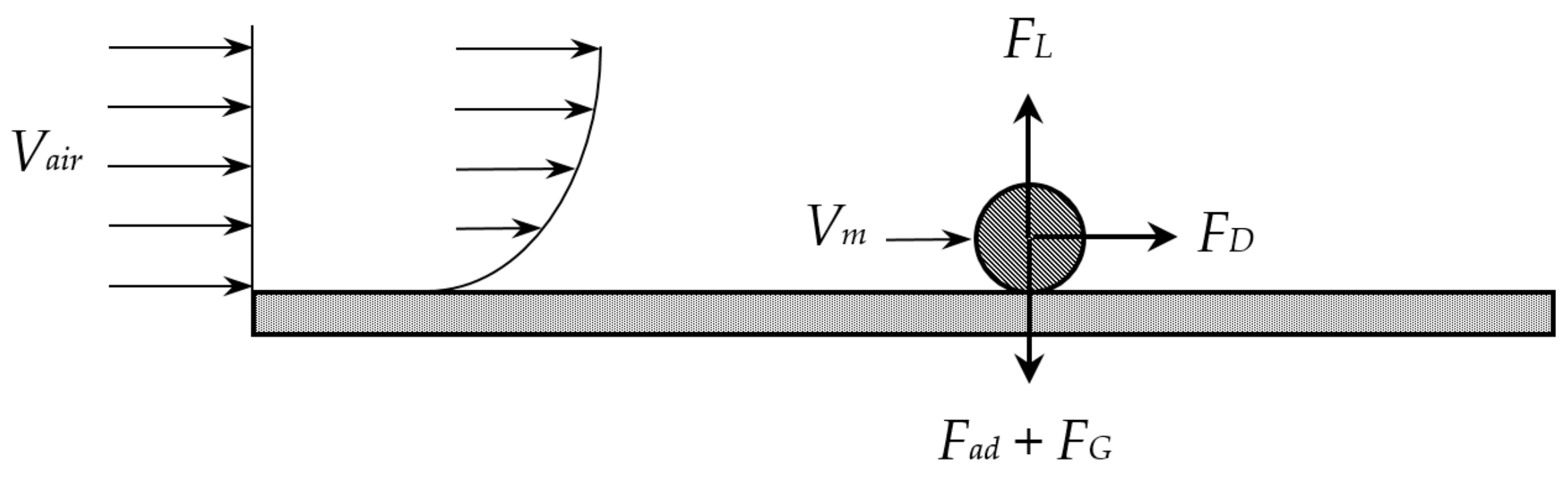
2.1.7. PV Panel Cleaning

To model the benefits of cleaning, particles are assumed to be uniformly distributed on a smooth panel surface of uniform particle diameter. When dust is present on the surface of the panel, solar radiation is blocked from reaching the photodiodes so a reduction in electrical power output is observed. The cleaning model is adapted work presented for mathematically modelling the cleaning of solar PV panels from Li et al. [23]. The modelling approach assumes that the air blows uniformly across the entire surface of the panel with all areas cleaned evenly and subject to the same air velocity.

Particles adhere to the surface of the panels by three primary forces, the van der Waals forces, F_vdW; electrostatic forces, F_E; and capillary forces. As capillary forces arise from the presence of water, these are removed from analysis because the panel is assumed to be generating electricity in an arid environment. The dominant forces acting on the dust particles are shown in Figure 3.

An expression for the van der Waals forces between the particle and the panel surface is given in Equation (34) [24]:

$$F_{VdW}=\frac{A_h{R}_p}{6H_0{}^2}$$

(34)

where A_h is the Hamaker constant, R_p is the radius of the particle, and H₀ is the shortest distance between the respective surfaces. Additionally, the electrostatic force is given in Equation (35) [25]:

$$F_E=\frac{q_p^{ 2}}{16\pi {ϵ}_0{R}_p{}^2}\left[\frac{1}{\left(\zeta +{\zeta }^2\right)\left(1+0.5\log \left(1+\frac{1}{\zeta }\right)\right)}\right]$$

(35)

where q_p is the charge of the particle, ε₀ is the vacuum permittivity, and ζ is the ratio between the closest distance and the radius. As such, the total force with which the particle adheres to the panel surface is given by Equation (36):

$$F_{ad}=F_{vdW}+F_E$$

(36)

The particles can be removed as a result of the air blowing at high velocity over the panel. This generates a drag force, F_D; a lift force, F_L; and a rolling moment, M_R, on the particle. The shear velocity, V_sh, at the surface of the panel is calculated from the free stream velocity, V_air, and the surface correction factor C_f:

$$V_{sh}=\sqrt{\frac{C_f{V}_{air}{}^2}{2}}$$

(37)

where:

$$C_f=0.0592{\left(\frac{V_{air}L}{2}\right)}^{-0.2}$$

(38)

The shear velocity can be used to determine the mean air velocity, V_m, at the particle centre:

$$V_m=\frac{\mathsf{\Gamma }{R}_p{V}_{sh}^{ 2}}{\nu }$$

(39)

where Γ is the coefficient of the wall condition, and ν is the kinematic viscosity of the blowing air. The resultant drag force from an air stream is therefore given by Equation (40):

$$F_D=\frac{1.7C_D{\rho }_{air}\pi R_p{}^2{V}_m^2}{2C_{cu}}$$

(40)

When C_D is the drag coefficient, f is the wall correction factor, ${\rho }_{air}$ is the air density, V_m is the mean air velocity at the particle centre, and C_cu is the Cunningham correction factor [26]. The coefficient of drag is given as a function of the Reynolds number of the particle, Re_p [27]:

$$C_D=\left\{\begin{array}{c}\frac{24}{R{e}_p}\left(1+\frac{1}{6}R{e}_p{}^{2/3}\right), R{e}_p\le 1000\\ \\ 0.44, 1000<R{e}_p\le 2\times {10}^5\end{array}\right.$$

(41)

where

$$R{e}_p=2\mathsf{\Gamma }{\left(\frac{R_p{V}_{sh}}{\nu }\right)}^2$$

(42)

and

$$C_{cu}=1+\frac{\lambda }{R_p}\left(1.257+0.4\exp \left(-1.1\frac{R_p}{\lambda }\right)\right)$$

(43)

where λ is the molecular mean free path in the gas. Additionally, the rolling moment as a result of the air jet is given by Equation (44):

$$M_R=\frac{8\mathsf{\Gamma }{f}_m{\rho }_{air}\pi R_p{}^3{V}_{sh}^{ 2}}{C_{cu}}$$

(44)

and the resultant lift force is given as

$$F_L=\frac{11.904{\rho }_{air}{R}_p{}^4{V}_{sh}^{ 4}}{{\nu }^2}$$

(45)

Furthermore, gravity is acting upon the particle and contributes to the adhering of the particle upon the surface of the panel:

$$F_G=\frac{4\pi R_p{}^3{\rho }_{d}g}{3}$$

(46)

where ρ_d is the density of the dust particles, and g is gravitational acceleration.

There are three detachment conditions for the particles when blown by an air jet: they can either roll, lift away, or slide. These conditions are met when the resultant forces exceed the movement criteria given in Equations (47)–(49):

$$F_L\ge F_{ad}+F_G$$

(47)

$$F_D\ge \mu \left(F_{ad}+F_g-F_L\right)$$

(48)

$$F_D{\left(R_p{}^2-R_r^2\right)}^{1/2}+M_R \ge \left(F_{ad}+F_G-F_L\right)R_r$$

(49)

where R_r is the radius of the particle contact area. Therefore, if the air velocity is sufficiently high, the dust present on the surface of the panel is removed and a power improvement to the panels is observed.

The overall power loss factor, F, arising from soiling can be seen as

$$F=1-\frac{m\left(E_{abs}+{\beta }_f{E}_{scat}\right)}{A}$$

(50)

where m is the mass of dust present on the surface on the panel, E_abs is the absorption efficiency of the deposited particles, and E_scat is the scattering efficiency with β_f being the particle up-scatter fraction.

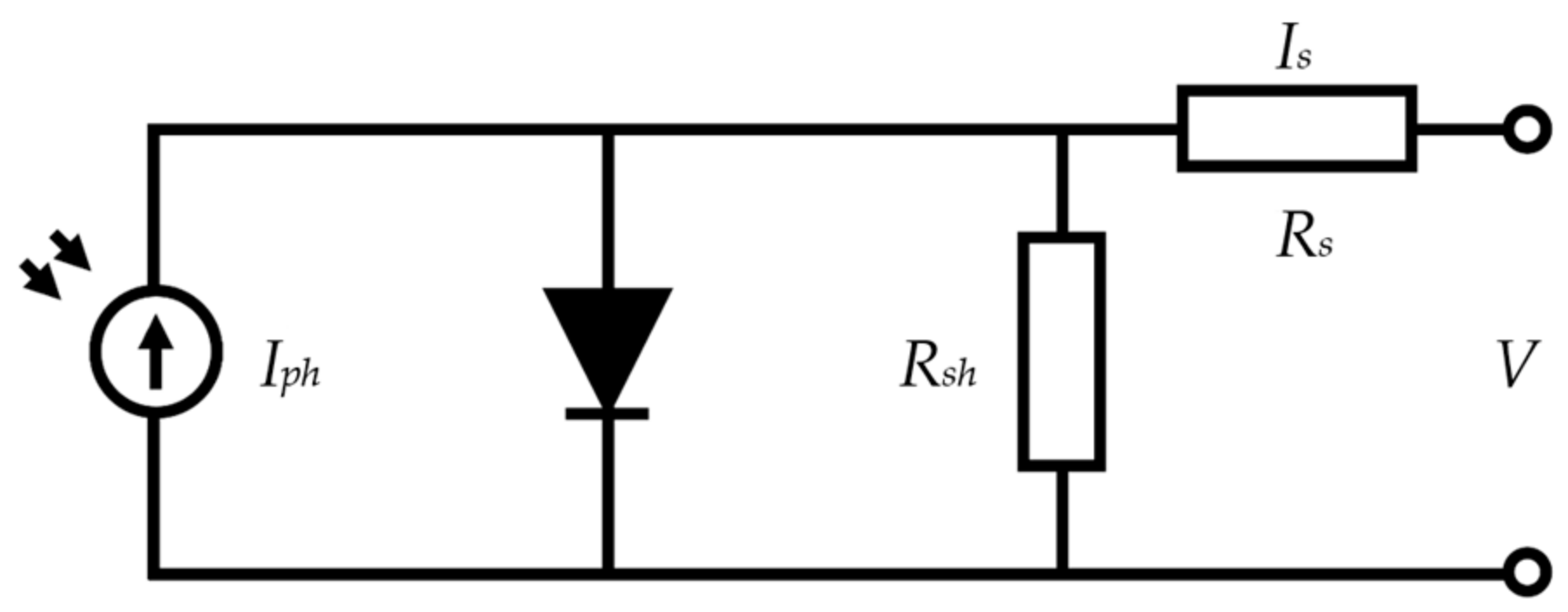
2.1.8. PV Panel Generation

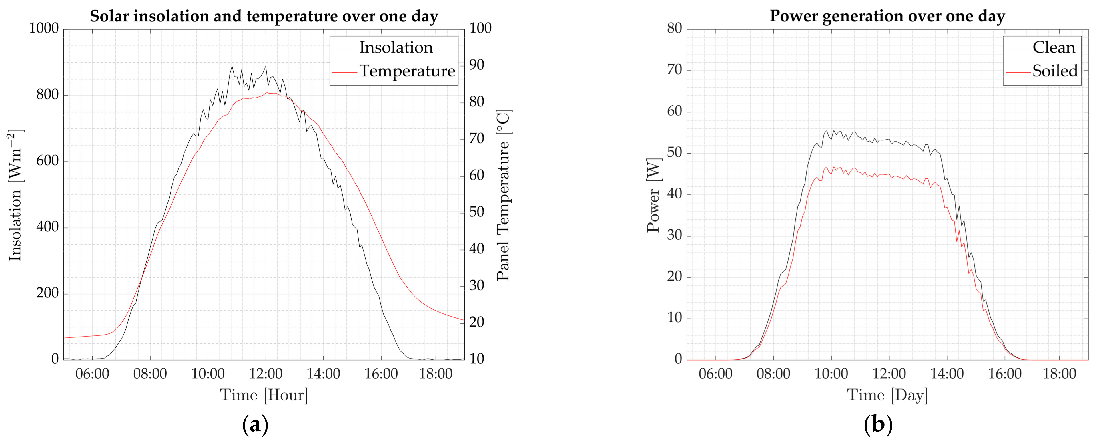
A PV module can be represented as a simplified circuit comprised of a photodiode as a current source within a single diode circuit [28,29]. This is shown in Figure 4.

The photocurrent, I_ph, is determined as a function of the short circuit current, I_sc; the short-circuit temperature coefficient, K_i; the cell temperature, T_p; the cell reference temperature, T_ref; and the solar irradiance, G, falling on the photodiode. This is given in Equation (51):

$$I_{ph}=\frac{G\left[I_{sc}+k_i\left(T_p-T_{ref}\right)\right]}{1000}$$

(51)

The diode saturation current, I₀, is a function of the reverse-saturation current, I_rs; cell temperature and reference temperature; electron charge constant, q; semiconductor band gap energy, E_g0; the diode ideality factor, n; and the Boltzmann constant, K_b, shown in Equation (52).

$$I_0=I_{rs}{\left(\frac{T_p}{T_{ref}}\right)}^3\exp \left[\frac{q{E}_{g0}\left(\frac{1}{T_{ref}}-\frac{1}{T_p}\right)}{n{K}_b}\right]$$

(52)

The reverse-saturation current is calculated given the short-circuit current; electron charge constant; open circuit voltage, V_oc; diode ideality factor; number of cells in series connection, N_s; Boltzmann constant; and cell temperature. This relationship is described by Equation (53):

$$I_{rs}=\frac{I_{sc}}{\exp \left[\frac{q{V}_{oc}}{n{N}_s{K}_b{T}_p}\right]-1}$$

(53)

The current through the shunt resistor, I_sh, is determined from the voltage experienced by the load, V; the current through the load, I; the series resistance, R_s; and the shunt resistance, R_sh. The relationship is given by Equation (54):

$$I_{sh}=\left(\frac{V+I{R}_s}{R_{sh}}\right)$$

(54)

Finally, the output current is given as a function of the photocurrent, saturation current, electron charge constant, voltage across the load, output current, series resistance, diode factor, Boltzmann constant, number of modules in series, cell temperature, and shunt current—given as Equation (55):

$$I=I_{ph}-I_0\left[\exp \left(\frac{q\left(V+I{R}_s\right)}{n{K}_b{N}_s{T}_p}\right)-1\right]-I_{sh}$$

(55)

3. Results

The subcomponents for the mathematical model presented in Section 2 are combined into a full-system mathematical model of the proposed PV-compressed air system and implemented in MATLAB/Simulink. A number of scenarios can be assessed to determine the potential benefit to PV generation from implementing the cooling and cleaning system from compressed air.

Solar irradiance data for a single December day in Kharagpur, India, are taken for analysis and used as input to the simulation; the solar data were measured locally using a reference cell-based irradiance sensor, recording at an interval of 5 min. The temperature achieved by a PV panel rated at 100 W under the conditions is modelled using the parameters contained in Appendix A. Additionally, with a fixed load of 45 Ω, the power output of the PV panel subjected to the input solar data is calculated. Furthermore, to demonstrate the modelling of soiling effects, a mass of 6 g of dust is deposited onto the surface of the panel and the power simulated again; this is equivalent to a typical soiling rate of 0.55 g m⁻² day⁻¹ for two weeks of exposure without cleaning. A particle size of 10 μm radius was implemented, as this is in the range of the common size of dust particles on soiled panels [30]. The parameters for the dust and soiling modelling are also contained in Appendix A. These results are given in Figure 5.

Observing Figure 5a, solar irradiance data for the day range from 0–900 Wm⁻² and are representative of a clear day with little variation from the standard expected daily profile. The modelled peak temperature of the unsoiled PV panel mimics the profile of the solar generation but is offset with the peak temperature occurring later than the peak solar value. The range of temperature of the PV panel is from 16 to 82 °C. The effects of the panel soiling can also be seen from the simulation results shown in Figure 5b. For the fixed load of 45 Ω, the peak power for the clean panel is 56 W, whereas the 6 g of dust present on the panel surface reduces the peak power to 47 W, a reduction of 16.1%. This difference in power output between the two presented cases is the maximum that can be recovered from cleaning the panels. Note that maximum power point tracking (MPPT) is not employed in the simulation; therefore, the PV panel does not reach the peak power for the available irradiance. Additionally, the temperature effects on the panel also contribute to the peak power being less than the rated power of 100 W.

With the soiling and temperature modelling established, it is of interest to determine the optimum time for blowing and the duration of blowing that will give the greatest power improvement to the PV generation for a given amount of compressed air. When in possession of a fixed volume of compressed air at a fixed pressure, there are a number of discharging strategies that could impose different effects upon the panel. Utilising a higher discharging flow rate results in greater velocity air blowing over the panels but reduces the blowing duration because the stored air is discharged faster. Conversely a smaller flow rate will result in slower velocity air blowing over the surface of the panel but for a longer duration. The demonstration of this effect can be seen in Figure 6, where a single 340 L tank at 5 bar pressure is used for study.

The balance between blowing duration and blowing velocity and the relative benefits to the PV panel generation is therefore of interest, as is considering at what point during the day to discharge the air because the temperature profile of the panel varies throughout the day. The total energy generation from one PV panel over one day was used as the metric for assessing the increase in performance from the different discharging conditions. The same solar profile and input parameters as used for Figure 5 were used for the simulation, as was the single air tank at 5 bar. The study for assessing the cleaning and cooling benefits was undertaken for a soiled and clean panel. The results can be seen in Figure 7.

Figure 7a demonstrates the simulation result of the cleaning and cooling for a soiled panel. The solar data for the same day are used multiple times for simulations, first varying the flow rate of air blowing over the panel and secondly varying the time at which the air is blown. The total energy captured by the single panel is measured for the day; this is the integral of the power of the panel. It is clear that to capture the most energy, blowing the air, and therefore cleaning the panel, is most effective when conducted earlier in the day. This gives the greatest length of time that the clean panel surface can absorb solar radiation unblocked by dust particles. The overall difference in energy capture from the single day ranges from 0.284 to 0.337 kWh for the panel of study, depending on the time of day the air was discharged. Additionally, for the established parameters, the lowest flow rates and corresponding slower air velocities were sufficient to remove the dust with the specified particle radius from the panel’s surface. The flow rate and air velocity do not greatly impact the total energy generation in the soiled case, as the soiling effects are greater than the temperature effects.

A clean panel is assessed in the second scenario, presented in Figure 7b. The increase in captured energy from the PV panel in these analyses only accounts for the benefits from the cooling of the panel from the compressed air flow. A larger amount of energy is captured when the panel is cooled during the periods when solar radiation is greater around solar noon. Additionally, a larger flow rate, corresponding to a shorter blowing duration and a faster velocity air, achieves a greater energy improvement. This is because a faster blowing speed creates a greater temperature drop in the panel for a shorter duration. This strategy therefore provides a larger energy benefit than a smaller temperature drop for a longer duration. The range of energy capture for the different scenarios is from 0.337 to 0.350 kWh.

The difference in energy capture from these different scenarios of the cleaning and cooling system can be observed in Figure 8.

Figure 8 indicates the difference in performance from the single PV panel of study under the same input solar radiation for different scenarios over a one-day period. The clean panel subject to cooling, is cooled at the optimum time to achieve maximum energy capture, according to the analysis demonstrated in Figure 7b, at solar noon. The soiling rate is again set to 14 days of soiling as previously indicated. Cleaning effects from the compressed air system can be seen to contribute the most to increasing energy capture: an 18.7% increase from a soiled panel, with cooling at the optimum time additionally creating a further 3.7% increase or a 23.2% increase from the soiled and non-cooled panel. It can be seen that in this instance, the removal of dust from the panel results in a greater improvement to energy generation than the cooling of the panel.

These results, along with the mathematical models of the other subsystem components, can be used to determine the potential energy return on investment (ROI) from the implementation of such a system. The energy ROI, ROI_E, gives an indication of improvement in performance across a fixed period for the proposed system and is calculated with (56):

$$RO{I}_E=\frac{E_{CC}-E_S}{E_{COMP}}$$

(56)

where E_CC is the energy captured from the PV generation across a period when the system has been in operation, E_S is the energy from the PV panel across the same period and conditions without the system in operation, and E_COMP is the energy required for the compression of air that is used for cleaning and cooling. The energy required to compress the air is calculated using the motor and compressor modelling contained in Section 2 and the parameters contained in Appendix A. The time period for which to assess the energy ROI is chosen as 14 days, because of the soiling rate that has been established; after a 14-day soiling period, the panel has the same amount of dust on the surface as prior to cleaning on the first day. These results are given in

Table 1. Energy ROI for 14 days of PV generation.

Energy, Clean ECC [kWh]	Energy, Soiled ES [kWh]	Energy Difference [kWh]	Compressor Energy ECOMP [kWh]	Energy ROI
4.7137	4.2608	0.4529	0.019	23.8

and Figure 9.

As with the previous cases, the simulation consists of a single air tank used to clean the panel; this is performed on the first day of study. The power generation over 14 days can be observed in Figure 9, which also displays the power generation from the panel over a 14-day period if the panel is uncleaned. The panel soiling rate was again set to 0.55 g m⁻² day⁻¹ with the initial mass set at 14 days of soiling at this rate. The difference in power generation during this time is determined. An energy ROI arising from the cleaning of the panels from the system is calculated as 23.8. This is almost entirely from cleaning, as recurring cooling is not conducted during the two-week period. To provide additional efficiency improvement from cooling, the compressor would need to continuously operate; this would significantly lower the overall energy ROI because of the consumed energy driving the compressor. A further strategy needs to be developed to optimize the energy gains from cooling. Implementing the cleaning strategy and achieving a large ROI from cleaning additionally eliminate the need for regular manual cleaning. Additionally, variation of air pressure and store sizes would have an effect on the energy ROI of the system. A larger air store and higher air pressures would allow for greater flow rates and blowing durations, as well as more flexible or recurring operation, but would therefore require significantly more energy to compress the air. The optimization of the air store size and pressure, therefore, needs to be undertaken.

4. Conclusions

A mechanism for improving the efficiency of solar PV generation has been proposed by integrating a compressed air system. The compressed air can be used for panel cleaning and cooling by directing the high-pressure air through piping and nozzles to blow over the panel surfaces. The air streams will remove dust present on the panels and additionally provide a convective cooling effect, lowering the panel temperatures. The actions of both cleaning and cooling improve the power generation of PV modules.

The system has been outlined, and the constituent components have been discussed with the mathematical models of each derived. Initial simulation results indicate the benefit to PV generation that high-pressure air for cleaning and cooling can create. Scenarios examining the power generation of a single PV panel have been simulated, subject to different air blowing durations, speeds, and times. It is concluded that for a heavily soiled panel, cleaning with air as early as possible in the day is advantageous for the greatest energy capture. Alternatively, if the PV module has recently been cleaned, the greatest benefit to the power improvement by cooling occurs when a high flow rate is used at a time when solar insolation is most abundant. It is concluded that the action of cleaning PV modules provides a greater benefit to the power production of the PV modules than the cooling effects generated by the system. The simulation results indicate that a 23.2% increase in power production can be achieved when using the system when compared to the power production of a soiled panel over a one-day period.

Recommendations for Future Work

With the complete system model of the PV-compressed air system established, there are a number of future activities of interest. The model can be refined with the consideration of the velocity profile of the air across the panel. In this study, uniform air velocity and cleaning is assumed; thus, this can be enhanced with additional consideration of air behaviour. Furthermore, the current model assumes a uniform particle size distribution resulting in a uniform removal of the particles; to enhance the accuracy of the model, a distribution in particle size and density on the panel surface could be adopted. Thus, different size particles would require different velocities to detach, and full cleaning would not be achieved. MPPT can subsequently be added into the system to additionally identify the effects of cooling and cleaning to provide scope for further improving the efficiency of the integrated system. Additionally, different cooling and cleaning strategies will be investigated. In this study, a single fixed volume of compressed air at a constant starting pressure was assumed, and the best power improvement from this scenario was determined. The mathematical model can be used to determine the optimum size of components with regard to compressed air volume, installed PV capacity, etc., and the long-term operation of such a system must also be considered, as a single day is examined in this study. Finally, the model should be validated with different dust sizes and compared to experimental analysis to conclude the efficacy of the use of compressed air for the removal of dust.

References

1. International Renewable Energy Agency. The Power to Change: Solar and Wind Cost Reduction Potential to 2025; IRENA: Abu Dhabi, United Arab Emirates, 2016. [Google Scholar]
2. Reyes-Belmonte, M.A. Quo Vadis Solar Energy Research? Appl. Sci. 2021, 3015, 11. [Google Scholar]
3. International Energy Agency (IEA). Renewable Energy Market Update; IEA: Paris, France, 2020. [Google Scholar]
4. Maghami, M.R.; Hizam, H.; Gomes, C.; Radzi, M.A.; Rezadad, M.I.; Hajighorbani, S. Power loss due to soiling on PV panel: A review. Renew. Sustain. Energy Rev. 2016, 59, 1307–1316. [Google Scholar] [CrossRef] [Green Version]
5. Javed, W.; Guo, B.; Figgis, B.; Aïssa, B. Dust potency in the context of solar photovoltaic (PV) soiling loss. Sol. Energy 2021, 220, 1040–1052. [Google Scholar] [CrossRef]
6. Smestad, G.P.; Germer, T.A.; Alrashidi, H.; Fernández, E.F.; Dey, S.; Brahma, H.; Sarmah, N.; Ghosh, A.; Sellami, N.; Hassan, I.A.I.; et al. Modelling photovoltaic soiling losses through optical characterization. Sci. Rep. 2020, 10, 58. [Google Scholar] [CrossRef] [Green Version]
7. Sayyah, A.; Horenstein, M.N.; Mazumder, M.K. Energy yield loss caused by dust deposition on photovoltaic panels. Sol. Energy 2014, 107, 576–604. [Google Scholar] [CrossRef]
8. Bessa, J.G.; Micheli, L.; Almonacid, F.; Fernández, E.F. Monitoring photovoltaic soiling: Assessment, challenges, and perspectives of current and potential strategies. Iscience 2021, 24, 102165. [Google Scholar] [CrossRef]
9. Poulek, V.; Matuška, T.; Libra, M.; Kachalouski, E.; Sedláček, J. Influence of increased temperature on energy production of roof integrated PV panels. Energy Build. 2018, 166, 418–425. [Google Scholar] [CrossRef]
10. Santiago, I.; Trillo-Montero, D.; Moreno-Garcia, I.; Pallarés-López, V.; Luna-Rodríguez, J. Modeling of photovoltaic cell temperature losses: A review and a practice case in South Spain. Renew. Sustain. Energy Rev. 2018, 90, 70–89. [Google Scholar] [CrossRef]
11. Koehl, M.; Heck, M.; Wiesmeier, S.; Wirth, J. Modeling of the nominal operating cell temperature based on outdoor weathering. Sol. Energy Mater. Sol. Cells 2011, 95, 1638–1646. [Google Scholar] [CrossRef]
12. Yadav, V.; Suthar, P.; Mukhopadhyay, I.; Ray, A. Cutting edge cleaning solution for PV modules. Mater. Today Proc. 2021, 39, 2005–2008. [Google Scholar] [CrossRef]
13. Gupta, V.; Sharma, M.; Pachauri, R.K.; Babu, K.N.D. Comprehensive review on effect of dust on solar photovoltaic system and mitigation techniques. Sol. Energy 2019, 191, 596–622. [Google Scholar] [CrossRef]
14. Siecker, J.; Kusakana, K.; Numbi, B.P. A review of solar photovoltaic systems cooling technologies. Renew. Sustain. Energy Rev. 2017, 79, 192–203. [Google Scholar] [CrossRef]
15. Bayrak, F.; Oztop, H.F.; Selimefendigil, F. Experimental study for the application of different cooling techniques in photovoltaic (PV) panels. Energy Convers. Manag. 2020, 212, 112789. [Google Scholar] [CrossRef]
16. Peng, B.; Zhu, B.; Lemort, V. Theoretical and Experimental Analysis of Scroll Expander. In Proceedings of the International Compressor Engineering Conference, West Lafayette, IND, USA, 11–14 July 2016; p. 2450. [Google Scholar]
17. Emhemed, A.A.; Mamat, R.B. Modelling the Simulation for Industrial DC Motor Using Intelligent Control. Procedia Eng. 2012, 41, 420–425. [Google Scholar] [CrossRef] [Green Version]
18. Wang, J.; Yang, L.; Luo, X.; Mangan, S.; Derby, J.W. Mathematical Modeling Study of Scroll Air Motors and Energy Efficiency Analysis—Part I. IEEE/ASME Trans. Mechatron. 2011, 16, 112–121. [Google Scholar] [CrossRef]
19. Wang, J.; Luo, X.; Yang, L.; Shpanin, L.M.; Jia, N.; Mangan, S.; Derby, J.W. Mathematical Modeling Study of Scroll Air Motors and Energy Efficiency Analysis–Part II. IEEE/ASME Trans. Mechatron. 2011, 16, 122–132. [Google Scholar] [CrossRef]
20. Wang, J.; Wang, D.J.D.; Moore, P.R.; Pu, J. Modelling study, analysis and robust servocontrol of pneumatic cylinder actuator systems. IEE Proc. Contr. Theory Appl. 2001, 148, 35–42. [Google Scholar] [CrossRef]
21. Ullmann, A.; Kushnir, R.; Dayan, A. Thermodynamic Models for the Temperature and Pressure Variations within Adiabatic Caverns of Compressed Air Energy Storage Plants. J. Energy Resour. Technol. 2012, 134, 2. [Google Scholar]
22. Holman, J.P.; Lloyd, J. Heat Transfer, 10th ed.; McGraw-Hill: New York, NY, USA, 2010. [Google Scholar]
23. Li, D.; King, M.; Dooner, M.; Guo, S.; Wang, J. Study on the cleaning and cooling of solar photovoltaic panels using compressed airflow. Sol. Energy 2021, 221, 433–444. [Google Scholar] [CrossRef]
24. Leite, F.L.; Bueno, C.C.; da Róz, A.L.; Ziemath, E.C.; Oliveira, O.N., Jr. Theoretical Models for Surface Forces and Adhesion and Their Measurements Using Atomic Force Microscopy. Int. J. Mol. Sci. 2012, 13, 12773–12856. [Google Scholar] [CrossRef]
25. Crowley, J.M. Simple Expressions for Force and Capacitance for a Conductive Sphere near a Conductive Wall. In Proceedings of the ESA Annual Meeting on Electrostatics, Minneapolis, MN, USA, 17–19 June 2008. [Google Scholar]
26. Davies, C.N. Definitive equations for the fluid resistance of spheres. Proc. Phys. Soc. 1945, 57, 259. [Google Scholar] [CrossRef]
27. Ahmadi, G.; Guo, S. Bumpy Particle Adhesion and Removal in Turbulent Flows Including Electrostatic and Capillary Forces. J. Adhes. 2007, 83, 289–311. [Google Scholar] [CrossRef]
28. Nguyen, X.H.; Nguyen, M.P. Mathematical modeling of photovoltaic cell/module/arrays with tags in Matlab/Simulink. Environ. Syst. Res. 2015, 4, 24. [Google Scholar] [CrossRef]
29. Humada, A.M.; Hojabri, M.; Mekhilef, S.; Hamada, H.M. Solar cell parameters extraction based on single and double-diode models: A review. Renew. Sustain. Energy Rev. 2016, 56, 494–509. [Google Scholar] [CrossRef] [Green Version]
30. Pulipaka, S.; Kumar, R. Analysis of distortion factor for photovoltaic modules using particle size composition. Sol. Energy 2018, 161, 90–99. [Google Scholar] [CrossRef]
Figure 1. The proposed system is comprised of a DC motor which charges a scroll-type air compressor. Air accumulates in a storage tank and then can be discharged to blow air over the surface of PV panels. This action will clean and cool the panels.
Energies 14 04072 g001
Figure 2. (a) Geometry definition for the scroll compressor blades; (b) scroll-type air compressor blade geometry. The moving scroll orbits on a fixed path and is enveloped by the fixed scroll. Air is compressed as it moves inwards from the inlet to the central outlet valve.
Energies 14 04072 g002
Figure 3. Forces acting upon particles adhered to the panel surface when subjected to an air stream.
Energies 14 04072 g003
Figure 4. Single diode circuit representation of a PV module.
Energies 14 04072 g004
Figure 5. (a) Solar irradiance value and panel temperature of the clean PV panel over a one-day period; (b) power output from the PV panel over a one-day period.
Energies 14 04072 g005
Figure 6. The variation of blowing duration and flow velocity as a function of the set flow rate for a fixed volume and pressure of compressed air. A low flow rate corresponds to long duration, slow velocity blowing, and high flow rate corresponds to short duration, high velocity blowing.
Energies 14 04072 g006
Figure 7. The effects of blowing duration and time of blowing on the energy capture from a single PV panel. (a) Soiled panel; (b) clean panel.
Energies 14 04072 g007
Figure 8. The energy capture of the PV panel under different conditions.
Energies 14 04072 g008
Figure 9. Power from PV over 14 days for soiled and clean panels.
Energies 14 04072 g009