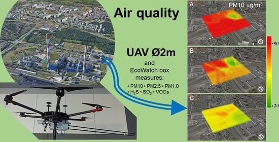
3D Spatial Analysis of Particulate Matter (PM₁₀, PM_2.5 and PM_1.0) and Gaseous Pollutants (H₂S, SO₂ and VOC) in Urban Areas Surrounding a Large Heat and Power Plant

Abstract

In many regions of the world, the winter period is a time of poor air quality, due primarily to the increased use of individual and district heating systems. As a consequence, the atmospheric air contains increased concentrations of both particulate matter and gaseous pollutants (as a result of “low” emissions at altitudes of up to 40 m and “high” emissions more than 40 m above ground level). In winter, the increased pollution is very often exacerbated by meteorological conditions, including air temperature, pressure, air speed, wind direction, and thermal inversion. Here, we analyze the concentrations of particulate matter (PM₁₀, PM_2.5, and PM_1.0) and gaseous pollutants (H₂S, SO₂, and VOC) in the immediate vicinity of a large solid fuel-fired heat and power plant located in an urban agglomeration. Two locations were selected for analysis. The first was close to an air quality measurement station in the center of a multi-family housing estate. The second was the intersection of two main communication routes. To determine the impact of “low” and “high” emissions on air quality, the selected pollutants were measured at heights of between 2 and 50 m using an unmanned aerial vehicle. The results were compared with permissible standards for the concentration of pollutants. Temperature inversion was found to have a strong influence on the level of pollutants at various heights, with higher concentrations of particulate matter registered at altitudes above 40 m. The source of PM, H₂S, and SO₂ pollutants was confirmed to be “low emission” from local transport, industrial plant areas, and the housing estate comprising detached houses located in the vicinity of the measuring points. “High emission” was found to be responsible for the high concentrations of VOC at altitudes of more than 40 m above the intersection and in the area of the housing estate.

1. Introduction

Air quality depends on the volume of pollutant emissions, the intensity and type of physico-chemical changes occurring in the atmosphere, and the large-scale movement of air pollutants. Pollutants occur in the air for natural reasons, independent of humans, and from anthropogenic sources. Anthropogenic pollutants occur at high concentrations in highly urbanized areas, where there is often high population density, and, thus, have a particularly negative impact on human health and quality of life. Increased levels of pollutants are mainly caused by “low emissions” [1], mainly from road transport and household and municipal waste, including from heating individual homes [2,3].

Among the most dangerous pollutants emitted into the atmosphere are particulate matter pollutants (PM₁₀, PM_2.5, PM_1.0) and gaseous pollutants: (sulphur dioxide, carbon dioxide, carbon monoxide, hydrogen sulphide, or odors) [4,5,6,7]. Particulate matter pollutants have a negative impact on human health, both directly by penetrating the body (causing allergies and lung diseases), and indirectly by acting as carriers for heavy metals, microorganisms, and bacteria [8,9]. In the European Union, the permissible dust concentration has only been defined for the PM₁₀ and PM_2.5 fractions (in accordance with Directive 2008/50/EC). There are no standards for the PM_1.0 fraction, which is increasingly considered the most dangerous type of dust pollution. The permissible level of PM₁₀ is 50 μg/m³ for the daily average and 40 μg/m³ for the annual average. For PM_2.5, the maximum limit is 25 μg/m³ (annual average). According to WHO recommendations, the daily average concentration of PM_2.5 should not exceed 25 μg/m³.

Gaseous pollutants are another dangerous category of emissions. For example, hydrogen sulphide is released into the atmosphere as a result of the activities of crude oil refineries, during natural gas purification, as well as by food processing and animal husbandry plants [10]. Other sources include deaeration, drainage and sewage systems in buildings [11]. Small concentrations of hydrogen sulphide in the air may cause only eye irritation, but at higher concentrations of 1400–2800 mg/m³ it can cause respiratory damage and, ultimately, respiratory arrest. At concentrations above 7000 mg/m³, hydrogen sulphide can cause death in seconds [12,13]. For this reason, the permissible level of hydrogen sulphide has been defined as 0.02 mg/m³ (daily average) [14]. According to the WHO [15], the concentration of hydrogen sulphide in the air should not exceed 0.15 mg/m³ (daily average), and exposure to average concentrations of 7 μg/m³ for more than 30 min should be avoided. Due to the ability of gaseous pollutants to more easily penetrate buildings, they present a significantly greater challenge than dust pollutants [16].

Volatile organic compounds (VOC) are a diverse group of organic chemicals that are ubiquitous in most urban environments. According to the EPA (The US Environmental Protection Agency) [17], the most common VOC emissions come from chemicals used in new furniture, paints, aromatic hydrocarbons, cleaners, wood, various fuels, copying and printing machines, perfumes, varnishes, and tobacco products [18]. Common VOCs include ethanol, formaldehydes, benzene, and acetone. Due to the variety of VOCs, there are no unified guidelines for the permissible levels of VOC in the outside air. For example, benzene is a Group 1 carcinogen (as classified by the International Agency for Research on Cancer) [19].

Another important pollutant is sulphur dioxide, which is highly toxic with a suffocating smell. It has a high specific gravity and high relative density, which causes it to slowly spread through the atmosphere. Sulphur compounds contribute to acidification of the environment. Sulphur dioxide emissions can be described as “seasonal”, since higher concentrations are observed in the heating/winter seasons, whereas in the vegetation/summer seasons the concentrations decrease. Sulphur dioxide is produced mainly by the combustion of solid and liquid fuels (e.g., coal, crude oil) contaminated with sulphur, in internal combustion engines, power plants, and combined heat and power plants. The largest proportion of sulphur dioxide comes from the fuel and energy industry—i.e., combustion processes in industry and combustion processes during energy production [20]. The amount of SO₂ introduced into the environment depends largely on the quality of the fuel. According to Directive 2008/50/EC [21], the permissible average daily concentration of SO₂ is 125 µg/m³ and the average hourly concentration is 350 µg/m³. These levels are the acceptable values for the protection of human health. On the other hand, the WHO [22] has set a much lower value for the permissible average daily concentration of SO₂ at 20 µg/m³.

Air can transport pollutants over long distances. Rough terrain and dense agglomerations of buildings constitute a barrier that causes the accumulation of pollutants. This is combined in some cities with the development partial or complete urban ventilation corridors, which additionally increase levels of local pollution. As a consequence, dense and tall buildings are sometimes responsible both for increased levels of harmful substances in the air (especially in city centers) and for strong local air turbulence. There are also complex phenomena described by the theory of aerodynamics [23,24]. Models of pollution flow and spread in urban areas [25] have been created to reflect real phenomena and present information on how building affect the accumulation of pollutants. So-called street canyons where roads are surrounded by relatively tall buildings have been associated with the movement of pollutants [26,27]. The transport of pollutants is influenced by the layout and coefficient of the shape of streets, the geometry of the buildings, the source of pollution (height and location), and the direction and speed of the wind [25]. Due to the complexity of the phenomena and the number of parameters that should be taken into account, field studies are a very important source of information [28,29,30,31]. The purpose of this study was to determine spatial changes in the state of air pollution in a city in relation to sources of “low” and “high” emissions.

Currently, unmanned aerial vehicles are increasingly used for various purposes, such as mapping, transport, monitoring. The development and miniaturization of air quality measuring devices allowed the use of UAVs for their transport and measurement of pollutant concentrations in the air table [32,33,34]. Currently, research on this subject is carried out in many research centers. Most of them concern the stage of UAV and measuring equipment construction [35,36]. In the article, the authors present the previously unpublished use of UAV with measuring equipment, as well as the method of analyzing and interpreting the obtained results concerning 3D spatial air quality analysis.

2. Methodology

Measurement Area

Measurements were made in the city of Lodz, which is the third largest settlement unit in Poland (Central-Eastern Europe) in terms of the number of inhabitants (population 677,286, population density 2309.6 people/km²). The area of analysis covers the area of a municipal communication junction, which is located next to a large housing estate in the immediate vicinity of a solid fuel-fired heat and power plant. The critical points in this area are a housing estate with an air quality measurement station owned and run by the Voivodship Inspectors of Environmental Protection (VIEP) (Figure 1 point 1), the intersection of Puszkina street and Przybyszewskiego street (Figure 1, point 2), and the EC4 heat and power plant (Figure 1, point 3). The VIEP station (station ID: PL0096A) is a container station that automatically measures the parameters for PM₁₀, PM_2.5, and O₃. Around the air quality measurement station is an area of multi-family housing, characterized by a predominance of five-story residential buildings (15–20 m high) and a smaller number of 10-storey residential buildings (30–40 m high) (133,855 inhabitants, 1.45 km from the heat and power plant). The selected area allowed for the assessment of the impact of “low” and “high” emissions on residential areas. Moreover, the nearby air quality measurement station made it possible to verify the measurement results. The second critical point is an important north-south and east-west communication junction for residential and industrial areas, and an access point to the A1 motorway. It is a single-level intersection of multi-lane roads with two-lane circular traffic, located between the high emitter (EC4) and the air quality measurement point (VIEP station). The total measurement area is about 2 ha, surrounded from the north by collective housing estates and from the south by a cemetery, as well as industrial and commercial areas (in the north-south direction, 0.8 km from the main emitter of the heat and power plant). The second selected area, which is a communication node, made it possible to refer to linear emissions from road transport, and as the area of CHP plants located closer to it, it allows for the assessment of the direct impact of EC4 on pollutant emissions. The gross development intensity index for the area ranges from 0.05 to 1.0, which defines “the intensity of development of concentrated single-family housing, areas of large housing estates, areas of large industrial plants and areas of old suburban buildings”. Thus, both the VIEP station and the intersection are in the zone of influence of the pollutant emitter, i.e., the EC4 heat and power plant.

The EC4 power plant is one of two coal-fired CHP plants operating in the city of Lodz, producing electricity in a cogeneration system (thermal power 820 MW, electric power 198 MW). The main fuel used in EC4 is hard coal. The plant uses approximately 530,000 Mg/year of hard coal, in addition to 395,000 Mg/year of biomass and 400 Mg/year of light fuel. This translates into average emissions of 9.86 kg/h of PM₁₀, 4.23 kg/h of PM_2.5, and 250 kg/h of SO₂ (data from January to March 2019). The maximum average annual emissions from the plant of PM₁₀, PM_2.5 and SO₂ at 1.5 m above ground level are 0.013 μg/m³, 0.005 μg/m³, and 0.827 μg/m³, respectively.

Measurements were made at three levels (20, 35, and 50 m) above the intersection, using an DJI Matrice 600 Pro unmanned aerial vehicle (UAV) (MOT < 25 kg, diameter approximately 2 m) equipped with instruments for measuring particulate matter (PM₁₀, PM_2.5, PM₁) and gas pollutants (H₂S, SO₂, and VOC). The minimum height of 20 m was chosen to ensure safe flight conditions over the traffic route, street lighting, and tram lines. The maximum height of 50 m was prescribed by the controlled traffic region (CTR) around Wladyslaw Reymont airport in Lodz, located 9 km away. A grid of points was established in the area of the intersection, where the UAV made its measurements (Figure 2B).

The measurements at a height of 20 m reveal the state of air quality in the area of so-called “Low emission” (up to about 40 m relative height). The measurements taken at a height of 50 m represent the area of “high emissions”. In the vicinity of the measuring station (Figure 1, point 1), measurements were made at a height of 2 m, and then from 5 m to 50 m with a gradient of 5 m (Figure 2A).

The measurement apparatus was an eight-sensor module, which enabled the quantification of particulate matter and gaseous pollutants in the atmospheric air. Using a laser scattered (LS) sensor, the module measured PM₁₀, PM_2.5, and PM_1.0 (10,000 particles per second). Metal oxide semiconductor (MOS) type sensors measured the concentration of organic solvents (Ethanol, Iso-Butane, H₂, 0–500 ppm) and odors (0.5–1000 ppm isobutanol). ElectroChemical (EC) type sensors measured H₂S (3 ppb–1 ppm), O₂ (0.20–100%) and SO₂ (0.5–2000 ppm). The measuring apparatus was equipped with a probe, 1.5 m long, which eliminated the influence of the UAV on air turbulence and, therefore, any possible impact on the results (Figure 3).

Validation of the measurement data of particulate matter was performed on the basis of data from an accredited measuring station VIEP (the method equivalent to the reference method), while the gaseous pollutants were validated in relation to the VEGA-GC microchromatograph (equipped with a thermal conductivity detector TCD, minimum concentration of 500 ppb (0.005 ppm)). The analysis was based on the results of the parameters of particulate matter PM₁₀, PM_2.5, PM_1.0, as well as H₂S, SO₂ and VOC.

Measurement data from station (VIEP) was obtained from a publicly accessible internet database [37].

3. Analysis of Results

Data analysis was carried out using the ArcGIS Pro 2.6 program (Advanced license). Data containing the GPS coordinates of the measurement points from the measuring equipment were entered in the form of a vector layer in the EPSG: 2180 system. The frame of reference was changed to WGS 1984 Web Mercator for spatial analysis. The attributes of the points were the concentration values of the measured pollutant parameters. Using ArcGIS Pro software, the spatial distribution of pollutants was determined based on data interpolation. Interpolation was carried out using the Empirical Bayesian Kriging 3D method. The Kriging method has the advantage over other interpolation methods (Inverse Distance Weighting ‘IDW’, Triangulated Irregular Network ‘TIN’) that it treats the observed variable as a random variable [38,39]. The weighting factors are estimated by minimizing the sum of squared deviations for regression and using spatial autocorrelation (semi-variogram) of the examined feature. This improves the quality of spatial prediction.

4. Meteorological Conditions

Instantaneous measurements were made during the “winter period” (from 30 September 2020 to 1 April 2021). This period was chosen because it is commonly associated with increased air pollution, especially due to the combustion of solid fuels, especially hard coal. Poor air quality is one of the most significant problems in Polish cities (of the 50 most polluted cities in the EU, 36 are in Poland). The level of pollution in the “winter period” is strongly related to meteorological conditions, in particular air temperature, wind direction and wind strength. The analysis presented here focuses on three representative measurement series, taken on 11 December 2020 (series A), 18 December 2020 (series B), and 8 January 2021 (series C). The three series of measurements reflect typical conditions for the period. The measurements were all taken between 9:30 am and 12:00 am. During measurement series A and B, the weather conditions were similarly characterized by fog, low cloud cover, high relative humidity (above 80%), and average temperatures above 0. They differed in the direction of the wind. During series A, the wind was blowing from the south-east—i.e., from the EC4 pollutant emitter. During series B, a south-westerly wind predominated—i.e., from the side of the cemetery, industrial areas and single-family houses. Series C was selected for analysis because it showed a similar wind direction to series B, and a similar wind speed to series A. However, the weather conditions differed from those in both series A and series B. On the day of the measurements and on preceding days, there were freezing temperatures, frost, light snowfall, and a low and high base of cloud cover. Figure 4 shows photos of the weather conditions taken by the on-board UAV camera. The meteorological data are summarized in

Table 1. Statement of meteorological parameters (data source: www.meteoblue.com).

Series:	Parameters		Temp.	Relative Humidity	Total Precipitation	Total Cloud Cover	Wind Speed	Wind Direction
			[2 m above gnd]		(High resol.) [sfc]		[10 m above gnd]
	Unit		°C	%	mm	%	km/h	°
A	Min	9−12	−1.2	75	0	2.7	13.5	149
		24 h	−2.4	75	0	0	7.59	119
	Max	9−12	3.0	93	0	4.5	16.3	155
		24 h	3.4	97	0	100	16.3	191
	Average	9−12	1.2	81.8	0	3.8	15.5	151
		24 h	0.6	89.6	0	45.95	13.34	152
B	Min	9−12	3	93	0	62	3.6	220
		24 h	0	87	0	30	3.6	83
	Max	9−12	5	100	0	95	10.8	240
		24 h	5.2	98	15	95	10.8	237
	Average	9−12	4	96	0	78.5	5.9	230
		24 h	3.1	93.6	7.5	62.5	5.85	190
C	Min	9−12	−1.6	68	0	32	14.8	225
		24 h	−1.6	65	0	32	4.6	221.3
	Max	9−12	1	83	0	66	19.3	244
		24 h	1.3	94	0	100	25.5	270
	Average	9−12	−0.2	74.5	0	50.8	16.9	236
		24 h	−0.1	83.6	0	81.6	14.9	233.3

.

5. Results

Each series of measurements began at the voivodeship measuring station “1” (VIEP station). This was so that the values detected by its measuring equipment for PM₁₀ and PM_2.5 could be used as a reference (

Table 2. The difference between the measurement data and the data from the VIEP station.

Series		A		B		C
	Unit	PM10	PM2.5	PM10	PM2.5	PM10	PM2.5
VIEP station data	μg/m3	40	34	37.5	31.75	30	25.6
Measurement	μg/m3	43.7	31.4	40.9	31.6	31.5	25
Difference	%	−9.3	7.6	−9.1	0.5	−5.0	2.3

). The percentage difference between the data obtained from our measurements and those of the VIEP station did not exceed the permissible level of ±10%. The average for all series was approximately ±2%.

The measurements performed by the station also allowed us to observe changes in the air quality around the area of dense multi-family housing located about 1.45 km south of the EC4 emitter and industrial facilities. According to the Chief Inspectorate for Environmental Protection [37], a PM₁₀ level below 20 μg/m³ is very good; up to 50 μg/m³ is good; up to 80 μg/m³ is moderate; up to 110 μg/m³ is poor; up to 150 μg/m³ is bad; above 150 µg/m³ is very bad. The distribution of PM₁₀ pollution observed in series C was different from those observed in series A and B. The highest concentrations, reaching 38.4 µg/m³, were recorded at heights from 25 to 35 m above ground level. Above 35 m and below 25 m, the PM₁₀ concentrations were about 30% lower and ranged from 21 to 33 µg/m³.

The concentration of PM₁₀ pollutants in series A and B were found to exceed the permissible level of 50 µg/m³ at heights above 25 m (Figure 5). The concentrations of PM₁₀ were on average 8% higher in series A than in series B. The highest concentration was 66.5 µg/m³, which is 133% of the PM₁₀ standard. Closer to the ground (<25 m), in both series A and B the dust content in the air was also above the permissible standard, with 5-perc values as high as 40.7 μg/m³ (series A) and 37.7 μg/m³ (series B).

Figure 6 and Figure 7 show the measured concentrations of PM_2.5 and PM_1.0, which have much greater impact on human health. The concentration of PM_1.0 was only about 2–6% lower than the concentration of PM_2.5. During series A and B, high concentrations of these pollutants were measured at heights above 25 m. This is consistent with the measurement data for PM₁₀. At heights from 25 to 40 m, the average concentration of PM_2.5 was in the range of 30 to 43 μg/m³. Above 40 m, the PM_2.5 concentration was more than 45 μg/m³. The concentration of pollutants above 25 m was between 120% and 205% of the permissible PM_2.5 level of 25 μg/m³. Better air quality in terms of these pollutants was observed in series C. The highest concentrations of PM_2.5 and PM_1.0, at 28 and 27 μg/m³, respectively, were measured 20–30 m above ground level. Interestingly, the lowest concentrations of PM_2.5 were recorded above 45 m (21 μg/m³ on average). Below 10 m, the average was 25 μg/m³.

The results for particulate matter pollution in the area of the VIEP station can be explained by the temperature inversion occurring during series A and B. This phenomenon contributed to the formation of a low-suspended layer that prevented the pollutants from floating to the upper parts of the atmosphere. Based on the data in Figure 4, it is possible to estimate the height of the base of the inversion layer 100–130 m above the ground level. This causes a high concentration of PM pollutants at altitudes above 25 m. Lower concentrations of PM in the air layers below 25 m probably resulted from the presence in the measurement area of multi-family buildings with average heights of about 15–20 m and abundant greenery. In series A and B, it can be assumed that the sources of the dust pollution were low emissions (below 40 m), probably from single-family houses, industrial plants, and the main communication routes approximately 1.4 km away (Figure 8) (in the direction of the wind). Low emissions are mainly related to the heating season, as noted by Sówka [40]. In series A and B, the influence of the EC4 emitter on air quality can be excluded, because the chimney outlet is located at a height of 260 m, which is significantly above the temperature inversion layer. However, in the case of series C, there was no clear inversion layer. This translated into the presence of a noticeable air layer in the range of 20 to 30 m, characterized by lower concentrations of particulate matter pollutants. This was probably due to the formation of turbulence and the local transport of pollutants at the height of the roofs of the surrounding buildings. At higher altitudes, the pollutants dispersed, as evidenced by the fact the lowest concentrations in series C were recorded at heights above 40 m.

The concentrations of gaseous pollutants were also measured in the area of VIEP stations. No clear differences in concentration versus height were observed in any of the measurement series (

Table 3. Summary of measurement data for three series from the area of VIEP stations.

Series:	Parameters	PM10	PM2.5	PM1	H2S	SO2	VOC
	Unit	μg/m3	μg/m3	μg/m3	[ppm]	[ppm]	[ppm]
A	max	66.5	54.2	54.2	0.1580	0.7070	0.0020
	average	52.2	41.0	40.3	0.0235	0.0206	0.0003
	min	30.9	25.1	25.0	<min	<min	<min
	95-perc	63.6	52.1	51.4	0.1110	0.1530	0.0010
	5-perc	40.7	29.5	28.6	<min	<min	<min
B	max	61.6	54.6	54.6	0.1580	0.7070	0.0020
	average	48.4	41.2	40.6	0.0235	0.0194	0.0003
	min	28.4	25.3	25.2	<min	<min	<min
	95-perc	58.9	52.4	51.8	0.1110	0.1530	0.0010
	5-perc	37.7	29.7	28.8	<min	<min	<min
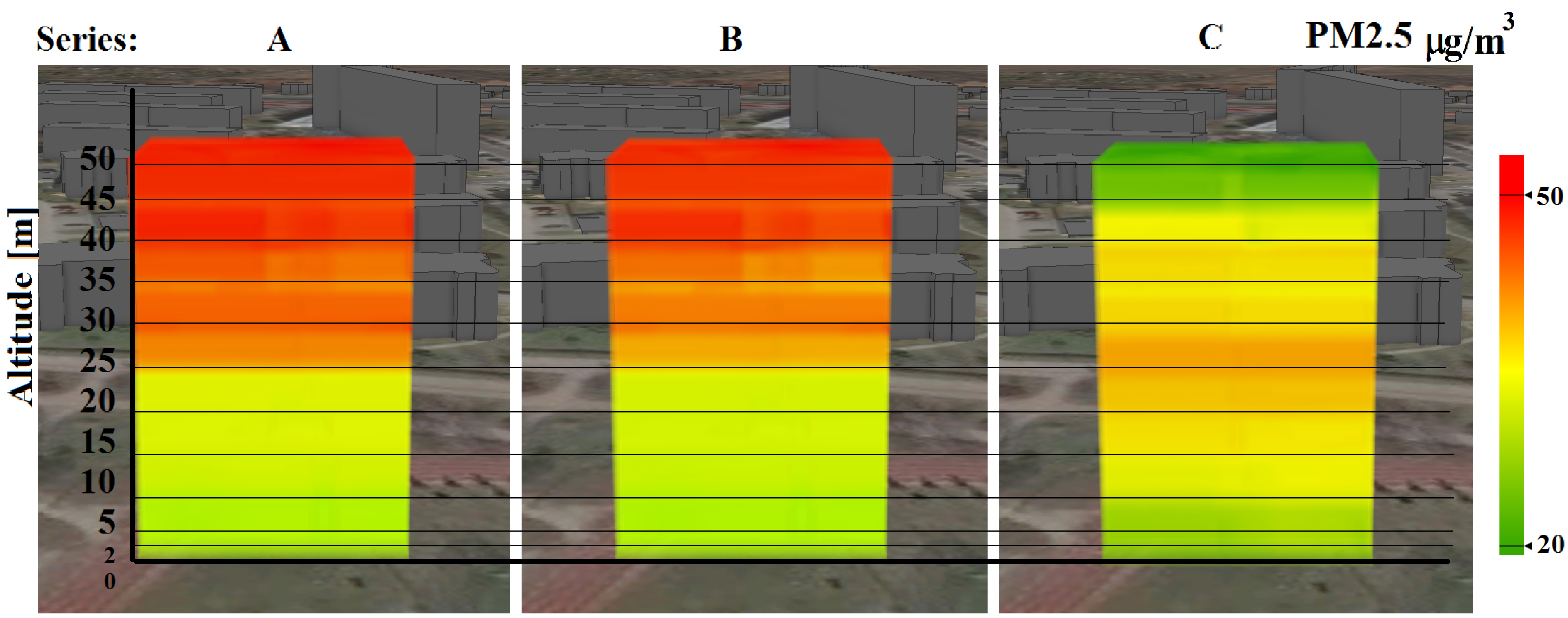
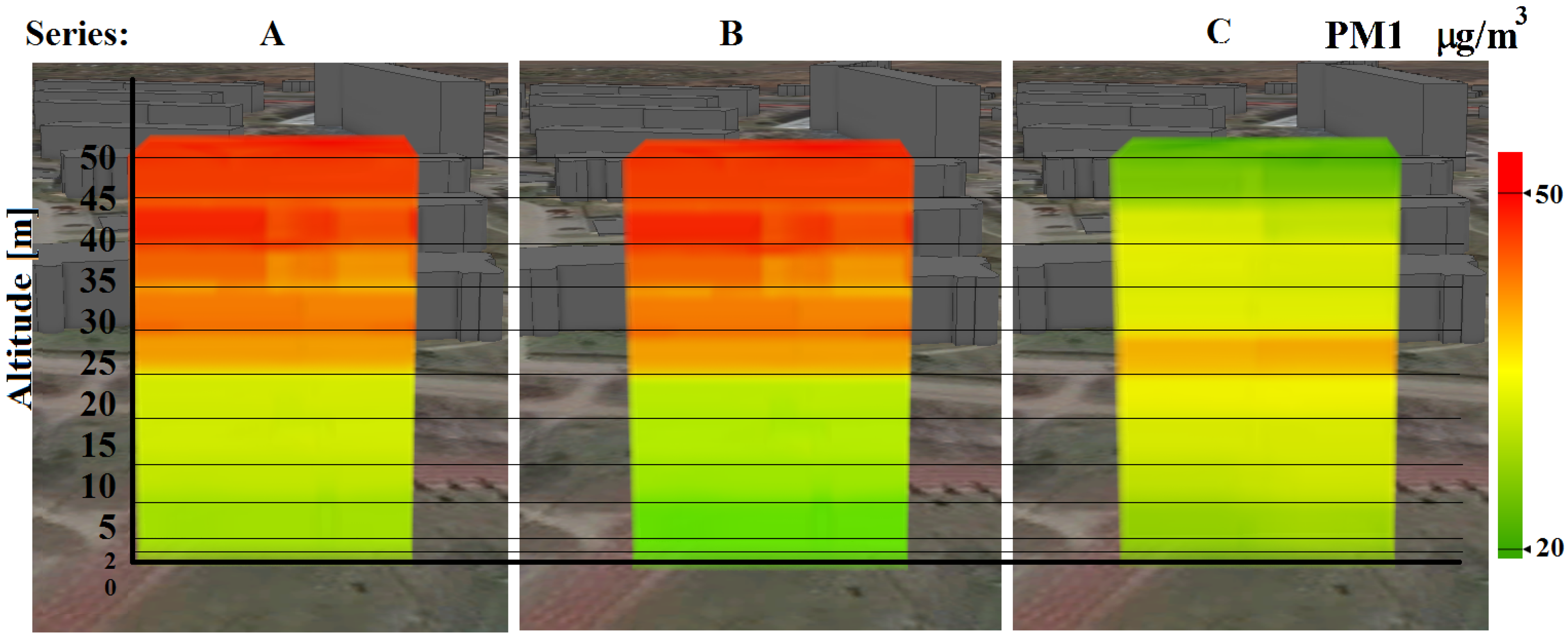
C	max	38.4	32.3	31.9	0.3280	0.8510	0.0030
	average	32.5	27.2	26.5	0.1172	0.0425	0.0010
	min	20.6	10.3	8.6	0.0030	<min	0.0010
	95-perc	36.3	31.5	31.0	0.2030	0.1460	0.0010
	5-perc	28.7	21.6	20.7	0.0320	<min	0.0010

<min—below the minimum excitation threshold of the measuring sensor.

). This was probably due to the distance of the measurement site from the main sources of gaseous pollutants, allowing them to mix with air. The only reproducible pattern was the increased concentrations of both hydrogen sulphide and sulphur dioxide at heights below 10 m, by up to 30% compared to the average value. This probably resulted from air stagnation caused by the presence of buildings in the measurement area. In all measurement series, the concentration of pollutants at many of the measurement points was below the minimum measuring threshold of the equipment. Only the average concentration of hydrogen sulphide significantly exceeded acceptable levels. In series A and B, the average concentration of hydrogen sulphide was about 0.036 mg/m³, which is 77% higher than the permissible value of 0.02 mg/m³. In series C, the concentration was as much as 750% of the permissible level, at 0.170 mg/m³, although it should be emphasized that this is significantly below lethal levels (1400 mg/m³). Overall, in series C the mean concentration of H₂S was five times higher than in series A and B and the concentration of SO₂ was twice as high. It can therefore be assumed that the results were influenced by the emission of pollutants from the EC4 CHP plant, especially since in series C there was no temperature inversion. The high concentrations of H₂S were likely emitted from the numerous vents from sewage systems in the densely packed residential buildings that surround the vicinity of the measuring station. This supports the results of previous research [11].

After the tests within the VIEP station, measurements were taken at the intersection of Puszkina street and Przybyszewskiego street. Clear changes were observed in the spatial distribution of the pollutants on the plane and with changes in height. For example, in series A the highest concentration of PM₁₀ (83 μg/m³) was measured at 50 m (average 63 μg/m³), whereas the lowest average (52 μg/m³) was measured at an altitude 35 m (Figure 9). Concentrations higher than 50 μg/m³ occurred in series A from the windward direction—i.e., from the open space side. On the opposite side of the intersection, where there are multi-family buildings and a larger number of trees, the concentration was up to 50% lower. The lowest concentration of PM₁₀ was recorded in the upper right corner of the area of analysis, where there are large numbers of trees and a green area. The influence of this area was visible even at a height of 50 m. An identical relationship was observed in the other series of measurements (B and C). In both series B and C the wind was blowing from the direction of the cemetery and industrial facilities. In both series (B and C), the average concentration of PM pollutants was 35% lower than in series A (

Table 4. Measurement data from the intersection area for three selected measurement series.

Series:	Parameters	PM10	PM2.5	PM1	H2S	SO2	VOC
	Unit	μg/m3	μg/m3	μg/m3	[ppm]	[ppm]	[ppm]
A	max	88.6	75.3	75.1	0.2110	0.9940	0.0110
	average	57.2	48.6	48.0	0.0387	0.1993	0.0022
	min	15.1	12.9	12.9	0.0010	0.0020	0.0005
	95-perc	82.8	70.4	70.2	0.1361	0.4951	0.0070
	5-perc	23.0	19.5	18.8	0.0043	0.0319	0.0005
B	max	55.5	49.9	49.2	0.0910	0.4610	0.0140
	average	38.5	30.8	30.1	0.0288	0.0993	0.0019
	min	12.2	5.5	4.8	0.0010	0.0010	0.0010
	95-perc	54.2	46.3	45.8	0.0570	0.3800	0.0050
	5-perc	19.2	8.7	7.5	0.0039	0.0010	0.0010
C	max	43.7	37.1	36.8	0.1050	0.3990	0.0160
	average	36.6	28.7	27.9	0.0395	0.1218	0.0035
	min	25.2	12.8	12.8	0.0010	0.0040	0.0010
	95-perc	41.0	35.1	34.6	0.0750	0.1894	0.0110
	5-perc	31.2	21.3	19.6	0.0040	0.0340	0.0010

). It can be assumed that this was due to the roughness of the terrain in the cemetery, which is covered with tall trees that trapped or accumulated the pollutants. In series A, the wind was blowing from the EC4 side, and probably transported particulate matter pollutants directly from the hard coal storage area. In series B, no significant differences (±2%) were found between the mean concentration of PM₁₀ at different heights. This was probably due to the wind speed, which was below 6 km/h and did not cause either violent air turbulence or PM₁₀ transport. The highest concentration of PM₁₀, about 40 μg/m³, was recorded in series B towards the boundary of the cemetery and the surrounding buildings. As noted in [41], buildings contribute to the accumulation of dust pollution on the leeward side. On the other hand, the lowest concentration of PM₁₀ (less than 30 μg/m³) was measured only in the green area around the intersection. Similar observations have been made with regard to the effect of traffic on the concentration of PM₁₀ [42].

In series C, the wind was almost three times stronger than in series B, and the influence of the buildings on the PM₁₀ concentration was even more visible (Figure 9). At a height of 20 m, the mean concentration of 40–50 μg/m³ was predominantly in the area sheltered by buildings, while average concentrations below 40 μg/m³ were measured only in the unprotected area. At a height of 35 m, practically the entire area of analysis was characterized by an average concentration of 40–50 μg/m³, probably due to the formation of vortices. At an altitude of 50 m, the PM₁₀ concentration dropped to below 40–30 μg/m³. This can be explained by the lack of thermal inversion in series C. In series A and B, when thermal inversion occurred, there was an accumulation of pollutants at higher altitudes.

The results for PM_2.5 and PM₁ were similar to those for PM₁₀ (Figure 10 and Figure 11). A strong correlation (>0.50) was found between the concentrations of the particulate matter pollutants. In series A, the highest concentration of dust pollutants at 75 μg/m³ was found windward from the heat and power plant and industrial areas, especially at a height of 50 m. Closer to the buildings, the PM content in the air fell by up to 40%, which may have been caused by the formation of vortices on the leeward side. As the measurement altitude decreased, the concentration of PM_2.5 and PM₁ fell by about 20% in comparison to the concentration at 50 m. This may indicate the accumulation of dust pollutants due to temperature inversion in the upper air layers. Peng [32] came to similar conclusions. In series B and C, the concentrations of PM_2.5 and PM₁ were about 30% lower than in series A. The content of pollutants in the air was below the permissible level of 25 μg/m³ only in the wooded area. In other places, the concentration of PM_2.5 exceeded the permissible level, reaching 175% of the permissible maximum. Gao [43] reported concentrations of PM_2.5 during the winter period reaching up to 500% of the limit defined in WHO guidelines.

Sources of gaseous pollutants include technological processes, fuel combustion and heavy transport. One of the contaminants analyzed was H₂S (Figure 12). High concentrations of H₂S were observed in series A, reaching 0.20 ppm (average 0.042 ppm) at a height of 50 m. At lower altitudes, the concentration decreased by 35% to an average value of 0.027 ppm at a height of 20 m. This can be explained by the wind direction and pollution accumulation due to thermal inversion.

In contrast to series A, in series B and C the highest concentrations of H₂S (over 0.06 ppm) were recorded at 20 m (Figure 12). This is consistent with the fact that H₂S is heavier than air and, therefore, accumulates near the ground. High concentrations of H₂S have also been observed near the ground by Cichowicz and Dobrzański [44]. An interesting phenomenon was the increased concentrations of H₂S at the exits of the intersection. This can be seen by comparing the maps of the H₂S distribution (Figure 12) in series A and B with the layout of the roads at the intersection. Given the temperature inversion in series A and B, it can be assumed that the H₂S in the air came from low emissions from the traffic rand industrial plants. Kourtidis et al. [45] suggest that a source of H₂S may be emissions from car catalysts. It is also possible to exclude the CHP as a source of H₂S, as in series C (no inversion) there was no increase in the concentration compared to series A and B. It should be emphasized that in all series the average concentration of H₂S was alarmingly high, exceeding the permissible level of 0.02 mg/m³. In series A, the average concentration was 0.058 mg/m³ (Table 4), which is almost 300% of the permissible level [14]. In series B, the average concentration was double the permissible level. In series C, it was about 40% higher than 0.02 mg/m³.

Another of the analyzed gas pollutants was sulphur dioxide, which is also heavier than air (Figure 13). In series B and C, high concentrations of SO₂ (more than 0.20 ppm, which is approximately 0.57 mg/m³) were measured at a height of 20 m. The average concentration fell at higher altitudes, by 17% and 25% in series B and C, respectively. However, in series A, where there was temperature inversion and a strong wind, the highest concentration (above 0.40 ppm) occurred mainly at a height of 50 m. Analyzing the area of the intersection, it can be seen that in series A and B there was a space with an increased SO₂ concentration compared to the surroundings. In series A, this is the exit from the intersection towards the city center, whereas in series B it is the exit from the intersection towards the residential part of the city. Note that these areas are in line with the direction air travel from the intersection. Interestingly, in the absence of thermal inversion (series C) no such relationship was observed. In most of the crossing area, the permissible SO₂ concentration of 0.35 mg/m³ was not exceeded. Only at the exits from the intersection was the permissible concentration of SO₂ exceeded, reaching about 130%. However, increased concentrations of SO₂ are usually observed in the winter [46], probably due to the increased production of thermal energy.

The final analyzed gas compound was VOC (Figure 14). There are no specific permissible levels for VOC. The distributions of VOC observed in series A and B were completely different to those in series C. Under the meteorological conditions in series A and B, with the visible influence of thermal inversion, a very low VOC concentration of less than 0.004 ppm (0.014 mg/m³) was recorded, but in most of the studied area the value was even lower, at less than 0.002 ppm. In series A and B, up to 50% higher concentrations were recorded at a height of 20 m, averaging 0.003 ppm at 35 and 50 m. The increased concentrations of VOC in series A and B were mainly associated with the communication routes, so the source of pollution was “local” low emission. The situation was completely different in series C (Figure 14), where the highest concentrations of up to 0.016 ppm (0.056 mg/m³) were found at an altitude of 50 m. However, at 35 m and 20 m the concentration of VOC decreased up to 7-fold. This may be evidence of the migration of VOC pollutants as a result of high emissions, although it would only be possible to test such a hypothesis under stable temperature gradient conditions.

6. Conclusions

This study set out to perform a spatial analysis of the distribution pollutants caused by “low” and “high” emissions. In series A and B, “low” emissions were associated with high concentrations of PM, SO₂ and H₂S at heights of 30–50 m. This was probably due mainly to the occurrence of temperature inversion. In series C there was no temperature inversion, which translated into lower concentrations of pollutants and a different spatial distribution to those in series A and B. The concentrations of pollutants were higher when temperature inversion occurred (Series A and B) than when there was no temperature inversion (Series C). This indicates that the emitters/chimneys of the coal-fired heat and power plant (EC4) had little effect on air quality in the analyzed area. It can be assumed that the EC4 CHP plant only contributed to high concentrations of VOC at altitudes above 40 m.

In series C, increased levels of suspended dust in the air were recorded at heights of 25 and 35 m above ground level. This may indicate an air corridor transporting PM pollution at this altitude. In all the measurement series, a strong correlation (above 0.5) was found between the PM₁₀, PM_2.5, and PM₁ dust fractions. A particularly high correlation coefficient (close to 1) was calculated for PM_2.5 and PM₁ (

Table 5. Correlation coefficient between measurement parameters from the intersection area for three measurement series.

	PM10	PM2.5	PM1	H2S	SO2	VOC
Series A
PM10	1.00	0.98	0.98	0.07	0.11	0.27
PM2.5	0.98	1.00	1.00	0.02	0.07	0.25
PM1	0.98	1.00	1.00	0.02	0.08	0.24
H2S	0.07	0.02	0.02	1.00	0.73	−0.17
SO2	0.11	0.07	0.08	0.73	1.00	−0.14
VOC	0.27	0.25	0.24	−0.17	−0.14	1.00
Series B
PM10	1.00	0.93	0.92	0.05	0.32	0.10
PM2.5	0.93	1.00	1.00	0.08	0.39	0.21
PM1	0.92	1.00	1.00	0.08	0.40	0.20
H2S	0.05	0.08	0.08	1.00	0.16	0.23
SO2	0.32	0.39	0.40	0.16	1.00	0.61
VOC	0.10	0.21	0.20	0.23	0.61	1.00
Series C
PM10	1.00	0.70	0.68	−0.06	−0.13	0.41
PM2.5	0.70	1.00	0.99	−0.02	0.01	0.22
PM1	0.68	0.99	1.00	−0.03	0.02	0.22
H2S	−0.06	−0.02	−0.03	1.00	0.43	−0.37
SO2	−0.13	0.01	0.02	0.43	1.00	−0.13
VOC	0.41	0.22	0.22	−0.37	−0.13	1.00

). Similar observations were made by Li et al. (2015), obtaining a correlation of 0.71–0.77 between PM. In all three series, concentrations of PM were measured that exceeded permissible values by up to 175% (PM_2.5). Presumably, this was related to season, with increased production of individual and industrial thermal energy during the winter period. In the housing estate, the concentration of gaseous pollutants remained the same in the height range from 2 to 50 m. This may be explained by turbulence from buildings, which mixed the gaseous pollutants with air, and by the distance from the source.

The measurements taken at the intersection of communication routes, located closer to the industrial areas, showed clear differences in terms of the distribution of gaseous pollutants at different heights. In the case of H₂S and SO₂, the distribution of concentrations was consistent with the road system and the orientation towards industrial areas. This indicates that these pollutants were caused by local low emissions. High VOC concentrations were only recorded at altitudes of more than 40 m within the intersection and housing estate areas in Series C (no temperature inversion), indicating that they originated from high emissions. The permissible level for H₂S was exceeded by up to 300% both in the area of the housing estate and at the intersection. The concentrations of H₂S were higher in the housing estate than in the area around the intersection. This was probably due to the numerous drainage vents located on the roofs of buildings on the housing estate. There was no clear correlation between the levels of gaseous pollutants in the three series. A weak correlation of 0.44 was found between H₂S and SO₂ levels in the three series. There was also no correlation between dust and gaseous pollutants (correlation coefficients below 0.5).

Summing up, the spatial analysis of pollutants with the use of UAVs gives the opportunity to get acquainted with the distribution of pollutants concentration in a selected area in detail. It should be emphasized that it is not possible to perform such measurements using traditional, stationary measuring stations located at a constant height from the ground, with a low spacing density. The method of measurement and analysis proposed by the authors can be implemented all over the world, therefore, it seems to be an important supplement to the existing methods of air quality measurement. The research methods presented in the article are now successfully used by us in air quality analyzes in various areas of Poland. The most important advantage of the obtained results is their high resolution in a small area, directly answering the question of air quality.

References

- Chlebowska-Styś, A.; Sówka, I.; Kobus, D.; Pachurka, Ł. Analysis of concentrations trends and origins of PM10 in selected European cities. In Proceedings of the 9th Conference on Interdisciplinary Problems in Environmental Protection and Engineering EKO-DOK, Boguszów-Gorce, Poland, 23–25 April 2017. [Google Scholar] [CrossRef] [Green Version]
- Jeong, C.H.J.; Jon, M.; Wang, J.M.; Greg, J.; Evans, G.J. Source apportionment of particulate matter in Europe: A review of methods and results. J. Aerosol. Sci. 2008, 39, 827–849. [Google Scholar]
- Zhao, Y.; Song, X.; Wang, Y.; Zhao, J.; Zhu, K. Seasonal patterns of PM10, PM2.5, and PM1.0 concentrations in a naturally ventilated residential underground garage. Build. Environ. 2017, 124, 294–314. [Google Scholar] [CrossRef]
- World Health Organization. Review of Evidence on Health Aspects of Air Pollution—REVIHAAP Project. World Health Organization 309. 2013. Available online: http://www.euro.who.int/en/health-topics/environment-and-health/air-quality/publications/2013/review-of-evidence-on-health-aspects-of-air-pollution-revihaap-project-finaltechnical-report (accessed on 1 February 2021).
- Moreno-Silva, C.; Calvo, D.; Torres, N.; Ayala, L.; Gaitán, M.; González, L.; Rincón, P.; Susa, M.R. Hydrogen sulphide emissions and dispersion modelling from a wastewater reservoir using flux chamber measurements and AERMOD® simulations. Atmos. Environ. 2020, 224, 117263. [Google Scholar] [CrossRef]
- Liu, N.; Liu, X.; Jayaratne, R.; Morawska, L. A study on extending the use of air quality monitor data via deep learning techniques. J. Clean. Prod. 2020, 274, 122956. [Google Scholar] [CrossRef]
- Edginton, S.; O’Sullivan, D.E.; King, W.D.; Lougheed, M.D. The effect of acute outdoor air pollution on peak expiratory flow in individuals with asthma: A systematic review and meta-analysis. Environ. Res. 2021, 192, 110296. [Google Scholar] [CrossRef] [PubMed]
- Pope Iii, C.A.; Burnett, R.T.; Thun, M.J.; Calle, E.E.; Krewski, D.; Ito, K.; Thurston, G.D. Lung cancer, cardiopulmonary mortality, and long term exposure to fine particulate air pollution. J. Am. Med. Assoc. 2002, 287, 1132–1141. [Google Scholar] [CrossRef] [Green Version]
- Dey, S.; Di Girolamo, L.; Van Donkelaar, A.; Tripathi, S.; Gupta, T.; Mohan, M. Variability of outdoor fine particulate (PM2.5) concentration in the Indian Subcontinent: A remote sensing approach. Remote. Sens. Environ. 2012, 127, 153–161. [Google Scholar] [CrossRef]
- Aventaggiato, L.; Colucci, A.P.; Strisciullo, G.; Favalli, F.; Gagliano-Candela, R. Lethal Hydrogen Sulfide poisoning in open space: An atypical case of asphyxiation of two workers. Forensic Sci. Int. 2020, 308, 110122. [Google Scholar] [CrossRef]
- Matos, V.R.; Ferreira, F.; Matos, S.J. Influence of ventilation in H2S exposure and emissions from a gravity sewer. Water Sci. Technol. 2020, 81, 2043–2056. [Google Scholar] [CrossRef]
- Fujita, Y.; Fujino, Y.; Onodera, M.; Kikuchi, S.; Kikkawa, T.; Inoue, Y.; Niitsu, H.; Takahashi, K.; Endo, S. A fatal case of acute hydrogen sulfide poisoning caused by hydrogen sulfide: Hydroxocobalamin therapy for acute hydrogen sulfide poisoning. J. Anal. Toxicol. 2011, 35, 119–123. [Google Scholar] [CrossRef] [Green Version]
- Stetkiewicz, J. Siarkowodór. Dokumentacja dopuszczalnych wielkości narażenia zawodowego. Podstawy I Metod. Oceny Środowiska Pracy. 2011, 4, 97–117. [Google Scholar]
- Polish Journal of Laws 1966: Regulation of the Council of Ministers of 13 September 1966 on Admissible Concentrations of Substances in the Atmospheric Air. Available online: http://isap.sejm.gov.pl/isap.nsf/DocDetails.xsp?id=WDU19660420253 (accessed on 10 September 2020).
- World Health Organization. Air Quality Guidelines, 2nd ed.; Hydrogen Sulfide: 2000, Chapter 6.6; Available online: https://www.euro.who.int/en/health-topics/environment-and-health/air-quality/publications/pre2009/who-air-quality-guidelines-for-europe,-2nd-edition,-2000-cd-rom-version (accessed on 1 February 2021).
- Wu, M.X.; Basu, R.; Malig, B.; Broadwin, R.; Ebisu, K.; Gold, B.E.; Qi, L.; Derby, C.; Green, S.R. Association between gaseous air pollutants and inflammatory, hemostatic and lipid markers in a cohort of midlife women. Environ. Int. 2017, 107, 131–139. [Google Scholar] [CrossRef]
- United States Environmental Protection Agency EPA. Available online: https://www.epa.gov/indoor-air-quality-iaq/volatile-organic-compounds-impact-indoor-air-quality (accessed on 12 September 2020).
- Hormigos-Jimenez, S.; Padilla-Marcos, M.Á.; Meiss, A.; Gonzalez-Lezcano, R.A.; Feijó-Muñoz, J. Ventilation rate determination method for residential buildings according to TVOC emissions from building materials. Build. Environ. 2017, 123, 555–563. [Google Scholar] [CrossRef]
- IARC. IARC (International Agency for Research on Cancer) Monographs on the Evaluation of Carcinogenic Risks to Human. 2016. Available online: http://monographs.iarc.fr/ENG/Classification/latest_classif.php (accessed on 10 December 2020).
- Meng, M.; Zhou, J. Has air pollution emission level in the Beijing–Tianjin–Hebei region peaked? A panel data analysis. Ecol. Indic. 2020, 119, 106875. [Google Scholar] [CrossRef] [PubMed]
- Directive 2008/50/EC of the European Parliament and of the Council of 21 May 2008 on Ambient Air Quality and Cleaner Air for Europe. OJ L 152, 11.6.2008, p. 1–44 (BG, ES, CS, DA, DE, ET, EL, EN, FR, IT, LV, LT, HU, MT, NL, PL, PT, RO, SK, SL, FI, SV) Special Edition in Croatian: Chapter 15. 2008, Volume 029, pp. 169–212. Available online: http://data.europa.eu/eli/dir/2008/50/oj (accessed on 6 July 2021).
- World Health Organization. Who Air Quality Guidelines for Particulate Matter, Ozone, Nitrogen Dioxide and Sulfur Dioxide. Global Update 2005. Summary of Risk Assessment; 2005; Available online: https://www.euro.who.int/en/health-topics/environment-and-health/air-quality/publications/pre2009/air-quality-guidelines.-global-update-2005.-particulate-matter,-ozone,-nitrogen-dioxide-and-sulfur-dioxide (accessed on 1 February 2021).
- Hosker, R.P. Flow around isolated structures and building clusters, a review. ASHRAE Trans. 1985, 91, 1672–1692. [Google Scholar]
- Pesic, D.; Zigar, D.; Anghel, I.; Glisovic, S. Large Eddy Simulation of wind flow impact on fire-induced indoor and outdoor air pollution in an idealized street canyon. J. Wind. Eng. Ind. Aerodyn. 2016, 155, 89–99. [Google Scholar] [CrossRef]
- Lateb, M.; Meroney, R.N.; Yataghene, M.; Fellouah, H.; Saleh, F.; Boufadel, M.C. On the use of numerical modelling for near-field pollutant dispersion in urban environments—A review. Environ. Pollut. 2016, 208, 271–283. [Google Scholar] [CrossRef] [PubMed] [Green Version]
- Murena, F.; Mele, B. Effect of short–time variations of wind velocity on mass transfer rate between street canyons and the atmospheric boundary layer. Atmos. Pollut. Res. 2014, 5, 484–490. [Google Scholar] [CrossRef] [Green Version]
- Kikumoto, H.; Ooka, R.A. numerical study of air pollutant dispersion with bimolecular chemical reactions in an urban street canyon using large-eddy simulation. Atmos. Environ. 2012, 54, 456–464. [Google Scholar] [CrossRef]
- Zhang, Y.; Kwok, K.; Liu, X.-P.; Niu, J.-L. Characteristics of air pollutant dispersion around a high-rise building. Environ. Pollut. 2015, 204, 280–288. [Google Scholar] [CrossRef]
- Zwack, L.M.; Paciorek, C.J.; Spengler, J.D.; Levy, J.I. Characterizing local traffic contributions to particulate air pollution in street canyons using mobile monitoring techniques. Atmos. Environ. 2011, 45, 2507–2514. [Google Scholar] [CrossRef]
- Galatioto, F.; Bell, M. Exploring the processes governing roadside pollutant concentrations in urban street canyon. Environ. Sci. Pollut. Res. 2013, 20, 4750–4765. [Google Scholar] [CrossRef] [PubMed]
- Rakowska, A.; Wong, K.C.; Townsend, T.; Chan, K.L.; Westerdahl, D.; Ng, S.; Močnik, G.; Drinovec, L.; Ning, Z. Impact of traffic volume and composition on the air quality and pedestrian exposure in urban street canyon. Atmos. Environ. 2014, 98, 260–270. [Google Scholar] [CrossRef]
- Peng, Z.-R.; Wang, D.; Wang, Z.; Gao, Y.; Lu, S. A study of vertical distribution patterns of PM2. 5 concentrations based on 410 ambient monitoring with unmanned aerial vehicles: A case in Hangzhou, China. Atmos. Environ. 2015, 123, 357–369. [Google Scholar] [CrossRef]
- Kalantar, B.; Mansor, S.B.; Abdul Halin, A.; Shafri, H.Z.M.; Zand, M. Multiple moving object detection from UAV videos 394 using trajectories of matched regional adjacency graphs. IEEE Trans. Geosci. Remote Sens. 2017, 55, 395. [Google Scholar] [CrossRef]
- Lambey, V.; Prasad, A.D. A review on air quality measurement using an unmanned aerial vehicle. Water Air Soil Pollut. 2021, 232, 1–32. [Google Scholar] [CrossRef]
- Xiong, X.; Shah, S.; Pallis, J.M. Balloon/Drone-Based Aerial Platforms for Remote Particulate Matter Pollutant Monitoring. 380 2018. Available online: https://scholarworks.bridgeport.edu/xmlui/handle/123456789/2236 (accessed on 1 February 2021).
- Jumaah, H.J.; Mansor, S.; Pradhan, B.; Adam, S.N. UAV-based PM2.5 monitoring for small-scale urban areas. Int. J. Geoinform. 2018, 14, 408. [Google Scholar] [CrossRef]
- Air Quality Parameters Data. Available online: https://powietrze.gios.gov.pl/pjp/current/station_details/table/295/3/0 (accessed on 8 May 2021).
- Singh, P.; Verma, P. A Comparative Study of Spatial Interpolation Technique (IDW and Kriging) for Determining Groundwater Quality. GIS Geostat. Tech. Groundw. Sci. 2019, 43–56. [Google Scholar] [CrossRef]
- Lima, A.; De Vivo, B.; Cicchella, D.; Cortini, M.; Albanese, S. Multifractal IDW interpolation and fractal filtering method in environmental studies: An application on regional stream sediments of (Italy), Campania region. Appl. Geochem. 2003, 18, 1853–1865. [Google Scholar] [CrossRef]
- Sówka, I.; Chlebowska-Styś, A.; Pachurka, Ł.; Rogula-Kozłowska, W.; Mathews, B. Analysis of Particulate Matter Concentration Variability and Origin in Selected Urban Areas in Poland. Sustainability 2019, 11, 5735. [Google Scholar] [CrossRef] [Green Version]
- Cichowicz, R.A.; Dobrzański, M. Indoor and Outdoor Concentrations of Particulate Matter and Gaseous Pollutants on Different Floors of a University Building: A Case Study. J. Ecol. Eng. 2021, 22, 162–173. [Google Scholar] [CrossRef]
- Rogula-Kozłowska, W.; Rogula-Kopiec, P.; Mathews, B.; Klejnowski, K. Effects of road trac on the ambient concentrations of three PM fractions and their main components in a large Upper Silesian city. Annals of Warsaw University of Life Sciences-SGGW. Land Reclam. 2013, 45, 243–253. [Google Scholar]
- Gao, J.; Wang, K.; Wang, Y.; Liu, S.; Zhu, C.; Hao, J.; Liu, H.; Hua, S.; Tian, H. Temporal-spatial characteristics and source apportionment of PM2.5 as well as its associated chemical species in the Beijing-Tianjin-Hebei region of China. Environ. Pollut. 2018, 233, 714–724. [Google Scholar] [CrossRef] [PubMed]
- Cichowicz, R.; Dobrzański, M. Spatial Analysis (Measurements at Heights of 10 m and 20 m above Ground Level) of the Concentrations of Particulate Matter (PM10, PM2.5, and PM1.0) and Gaseous Pollutants (H2S) on the University Campus: A Case Study. Atmosphere 2021, 12, 62. [Google Scholar] [CrossRef]
- Kourtidis, K.; Kelesis, A.; Petrakakis, M. Hydrogen sulfide (H2S) in urban ambient air. Atmos. Environ. 2008, 42, 7476–7482. [Google Scholar] [CrossRef]
- Cichowicz, R.; Wielgosiński, G. Analysis of Variations in Air Pollution Fields in Selected Cities in Poland and Germany. Ecol. Chem. Eng. 2018, 25, 217–227. [Google Scholar] [CrossRef] [Green Version]