Article

Surrogate-Based Optimization of Horizontal Axis Hydrokinetic Turbine Rotor Blades

by
David Menéndez Arán
* and
Ángel Menéndez
Laboratorio de Modelación Matemática, Departamento de Hidráulica, Facultad de Ingeniería, Universidad de Buenos Aires, Paseo Colón 850, Ciudad Autónoma de Buenos Aires C1063ACV, Argentina
*
Author to whom correspondence should be addressed.
Energies 2021, 14(13), 4045; https://doi.org/10.3390/en14134045
Submission received: 12 June 2021 / Revised: 28 June 2021 / Accepted: 1 July 2021 / Published: 5 July 2021
(This article belongs to the Special Issue Turbine Blade Optimization)

Abstract

:
A design method was developed for automated, systematic design of hydrokinetic turbine rotor blades. The method coupled a Computational Fluid Dynamics (CFD) solver to estimate the power output of a given turbine with a surrogate-based constrained optimization method. This allowed the characterization of the design space while minimizing the number of analyzed blade geometries and the associated computational effort. An initial blade geometry developed using a lifting line optimization method was selected as the base geometry to generate a turbine blade family by multiplying a series of geometric parameters with corresponding linear functions. A performance database was constructed for the turbine blade family with the CFD solver and used to build the surrogate function. The linear functions were then incorporated into a constrained nonlinear optimization algorithm to solve for the blade geometry with the highest efficiency. A constraint on the minimum pressure on the blade could be set to prevent cavitation inception.

1. Introduction

Horizontal axis hydrokinetic turbines (HKTs) are a class of energy conversion devices that transform the kinetic energy of flowing water into mechanical work. HKTs offer many advantages over conventional hydropower turbines due to their low set-up cost and environmental impact. The development of optimization tools for the design of efficient HKTs has therefore become a recent focus of worldwide research [1].
The operating principle of HKTs is largely equivalent to the one corresponding to horizontal axis wind turbines. However, there are also significant differences in the physics underlying both types of turbines, such as the density of the fluid medium, the potential for cavitation and biofouling [2,3], and the design of the support structure, among others.
Design and optimization techniques commonly used in the industry have been adapted from those developed for wind turbines and marine propellers. Blade Element Momentum (BEM) theory, commonly used for wind turbine design [4], has increasingly been applied to HKTs [5,6]. Lifting line theory was originally developed for the analysis and design of marine propellers [7], and it has recently been successfully extended to HKTs [8,9,10]. Both techniques are commonly used as preliminary design and analysis tools due to their high computational efficiency.
Lifting line models can also be used as the basis for mathematical optimization algorithms that seek blade loading distributions which maximize the torque generated by the rotor [8,9,10]. However, these models commonly adopt a series of simplifications that limit their capabilities as accurate predictors of turbine efficiency, such as constraints on wake geometry, assumptions on drag-to-lift ratios, and simplified hub geometries. The blade geometries generated with these methods are thus usually used as an initial step in an integrated design workflow including more sophisticated models such as vortex lattice [11,12], boundary element [11,12,13,14], and Computational Fluid Dynamics (CFD) models.
There is a spectrum of CFD models of varying complexity and fidelity that can be used to model HKTs, such as Large Eddy Simulation (LES) and Reynolds-averaged Navier–Stokes (RANS) models. LES models are usually reserved for modeling turbine wakes for turbine farm optimization [1,15,16], while RANS are commonly applied to accurately model horizontal axis wind turbines [17] and HKTs [18,19,20]. Unlike more simplified models, CFD simulations can directly consider non-uniform axial inflow conditions, flow separation, rotor-structure interaction, and viscous drag. However, the use of CFD greatly increases the computational cost of a given simulation. Optimization based on CFD simulations therefore requires efficient and robust methods to minimize the number of blade geometries that need to be analyzed.
The methodology presented in this article is based on steady-state RANS simulations using the open source multi-physics solver OpenFOAM [21] (version 8.0), seeking a compromise between accuracy and computational cost. A surrogate-based optimization (SBO) method [22] was selected to optimize the turbine rotor blade geometry. In this method, an approximate mathematical model (referred to as the “surrogate”) is constructed by sampling the design space and conducting a limited number of CFD simulations. Once the surrogate is built, it is used to replace the expensive CFD simulations for predicting the selected performance parameters (e.g., power coefficient).
A Multi-Objective Genetic Algorithm (MOGA) was selected to find the optimum blade geometry. The optimization algorithms and the interface between them and OpenFOAM were provided by the Dakota library [23]. Dakota is a general-purpose optimization toolbox developed by Sandia National Laboratories.
SBO has been used in the optimization of horizontal axis wind turbines [24] and marine turbines [25,26,27]. In general, previous research focuses on maximizing the power output of the turbine by varying a series of geometric parameters [25,26,27].
In this article, a preliminary geometry developed using an optimization method based on lifting line theory [9] was further optimized by means of multi-objective SBO. A turbine blade family was generated by multiplying a series of geometric parameters with the corresponding linear functions. A performance database was constructed for the turbine blade family with the OpenFOAM solver and used to build the surrogate function. The model results were used to characterize the design space and evaluate the influence of each design variable on turbine performance. The MOGA optimizer was finally employed to study the relationship between the power output, the thrust on the rotor, and the minimum pressure on the blade. Constrained optimization on blade pressure could then be set to prevent cavitation inception.

2. Methododology

2.1. Initial Geometry

2.1.1. Lifting Line Optimization

The lifting line optimization methodology used to generate the initial blade geometry is not the subject of this article, but it is briefly described in this section because it represents the starting point for the optimization method. Further details are given in [9].
Lifting line theory is particularly suitable for the high aspect ratio rotor blades commonly used for HKTs. Each blade is represented by a straight, radial line vortex of varying strength (bound vortex), characterized by the circulation Γ . The lifting lines extend from the hub to the blade tip and generate a more or less helical wake (free vortex sheet). One of the blades (referred to as the “key blade”) is selected for the analysis, and it is assumed that all the blades have the same circulation distribution. The bound vortex is then discretized into a series of horseshoe vortices of unknown strength Γ i , and a wake model is used to estimate the velocities induced on the key blade by the trailing vortex sheet.
For a known circulation distribution, the thrust T and torque Q on the key blade can then be estimated using the Kutta–Joukowski law. Viscous effects can be introduced into the formulation using a sectional drag-to-lift ratio κ = D / L [10], where D is the drag and L is the lift at a given section. The thrust and the torque can be expressed in nondimensional form as the thrust coefficient C T = T / 0.5 ρ π V 2 R 2 and the power coefficient C P o w = Q ω   / 0.5 ρ π V 3 R 2 , respectively, where V is the inflow velocity, ω is the rotor angular velocity, ρ is the water density and R is the rotor radius. The angular velocity is expressed nondimensionally as the tip-speed ratio T S R = ω R / V . These coefficients C P o w are commonly adopted as the key performance parameters for the turbine. The most efficient turbine will maximize power extraction ( C P o w ) while reducing the load on the rotor ( C T ) for a given operating condition ( T S R ).
Different optimization algorithms to maximize turbine torque (and consequently, power output) have been proposed. The classical theory can be adopted by assuming a constant-pitch wake with no deformation, known as Betz’s condition [10]. OpenProp [28] is an open-source lifting line code that can be applied for turbine rotor optimization, based on a hybrid lifting-line/momentum-theory procedure [8]. Other methods not using linear theory have been proposed, either by modeling the nonlinear terms when estimating the induced velocities on the key blade [29] or by combining the optimization algorithm with a full wake alignment model [9]. In general, all lifting line optimization algorithms are effective in producing highly efficient solutions [8,9,10,29], which indicates that for every combination of T S R and number of blades Z there exist a large number of solutions with high C P o w . Searching methods that attempt to find optimized geometries by varying HKT rotor blade geometric parameters [12,30] seem to sustain that conclusion.
The adopted wake model significantly affects the estimation of the power output for a given blade geometry [9]. The simplest wake model assumes that the horseshoe vortices follow a constant-pitch and constant-radius helical trajectory and that they are aligned to the velocity at the key blade [7,8]. More sophisticated models align the wake pitch angle at multiple sections downstream of the rotor [31] or employ force-free wake models that do not impose helical shapes and allow for the natural expansion of the wake [9], better resembling real HKT wakes, as predicted by RANS models. Complex wake models improve the accuracy of the power output prediction of lifting line models [31], yet their inclusion in the optimization algorithm presents a series of numerical challenges [9].
Lifting line models allow for quick parametric studies to determine the optimum TSR for different combinations of κ , Z , R , and hub radius R h u b . The results presented in this article assume Z = 3 , R = 1 m , R h u b = 0.2 m , and T S R = 5 , which maximizes C P o w according to lifting line optimization.

2.1.2. Initial Blade Geometry

For a given optimum circulation distribution Γ r , where r is the radial coordinate, the preliminary blade geometry can be created using Prandtl’s lifting line equation [7]. The circulation can be related to the sectional lift coefficient C L r by the Kutta–Joukowski law:
C L r = L i 0.5   ρ V * r 2   c r = 2   Γ r V * r   c r
where L is the sectional lift, c r is the chord distribution along the blade, and V * is the inflow velocity with respect to a blade-attached coordinate system. For a given chord distribution, Equation (1) can then be used to determine the lift coefficient.
The sectional pitch angle ϕ relates to the wake pitch angle β at the key blade and the sectional ideal angle of attack α i according to Equation (2).
ϕ r = β r α i r
The ideal angle of attack and the sectional maximum camber f m a x are a function of the lift as indicated in Equations (3) and (4). α 0 and f 0 are the ideal angle of attack and the ideal maximum camber when C L = 1 .
α i r = α 0   C L r
f m a x r = f 0   C L r
The generation of the blade geometry requires the selection of arbitrary radial maximum thickness and chord distributions and sectional mean line and thickness forms. Linear distributions, commonly used in the industry, are adopted for the maximum thickness chord. For this study, we have adopted typical sectional properties from the NACA series [32]. The 3D blade geometry can then be built from a sufficient number of 2D section profiles.
Hub effects are typically included in lifting line models by means of an image model [7], which represents the hub as a cylinder of infinite length. The geometry of the hub is heavily influenced by the design of the electromechanical components housed within it (e.g., generator, gearbox, etc.). A simple cylindrical geometry with rounded semispherical noses has been adopted for the present study. Some manufacturers build hydrodynamic hub shapes in order to reduce the drag transferred to the support structure.

2.2. Analysis

2.2.1. Model Set-Up

Performance assessment of the HKT rotor blade was conducted using the open source CFD library OpenFOAM [21,33]. OpenFOAM offers several numerical schemes to solve different terms of the fluid flow equations. It applies a segregated process using an iterative sequence coupling through well-known algorithms such as SIMPLE or PISO. To model the HKT, the steady-state, incompressible, isothermal, turbulent flow solver simpleFoam was used.
The RANS method of solution for the fluid flow equations was selected in order to attain a balance between acceptable solution accuracy and reasonable computational run times. The two-equation k-ω SST [34] turbulence closure model was adopted because it has been successfully applied to wind turbines [17] and HKTs [18,19,20] and has shown good agreement with experimental results [12]. The k-ω SST turbulence closure model requires the specification of values for the turbulence variables at the inlet. A sensitivity analysis to changes in the turbulence intensity from 1% to 10% was carried out, but no significant variation of the solution was detected.
The support structure was not included in the model, and the 120-degree periodicity of a three-bladed turbine allowed the simulation of only one third of the total domain, including a third of the hub and one of the rotor blades. The computational domain extended 10 R in the upstream direction, 30 R in the downstream direction and 10 R in the radial direction, where R is the rotor radius. Cyclic (periodic) boundary conditions were set on the symmetry planes, and free slip conditions on the far-field boundary. A uniform velocity field was imposed at the inlet, and a pressure outlet boundary condition at the outlet. A no-slip condition was specified at all hub and turbine surfaces.
The coordinate system used cartesian coordinates attached to the blade, with the x-axis as axis of rotation oriented in the direction of the flow, and the z-axis aligned with the blade. A rotating reference frame model with angular velocity ω was used to simulate the rotation of the blade and hub. This allowed the transformation of an unsteady flow problem when solved with respect to a stationary reference frame into a steady flow problem in the non-inertial moving frame.
The model domain and boundary conditions are represented in Figure 1.
Meshes were generated using the snappyHexMesh utility in OpenFOAM. The snappyHexMesh utility generates unstructured 3D meshes containing hexahedra (hexes) and split hexahedra from a triangulated surface geometry in Stereolithography (STL) format.
To generate a mesh with snappyHexMesh, a background or base mesh is required. The base mesh was generated using the blockMesh utility in OpenFOAM. The base mesh consisted purely of hexes, and the cell aspect ratio was approximately 1 in the region near the HKT. snappyHexMesh generates the final mesh by subdividing the base mesh locally as many times as necessary to achieve the desired cell size specified in each region of the domain. The resulting mesh is then fitted to the boundaries. Refinement regions were set near the HKT blade and in the wake region close to the rotor. Inflation layers were then added on the turbine and hub surfaces to improve mesh resolution in the boundary layer zones.
Due to the high number of simulations required, mesh density was selected as a compromise between model accuracy and computational run times. A mesh convergence analysis was carried out to evaluate the error and uncertainty in the estimation of the C P o w and C T coefficients due to mesh size.

2.2.2. Convergence Analysis

A convergence analysis using the Grid Convergence Index method (GCI) [35] was performed on the initial blade geometry described in Section 2.1.2. Three gradually refined nonstructured hex-dominant meshes with prismatic near-wall elements were used. These meshes were generated using the exact same method and parameters, but different element sizes on the base mesh were generated by the blockMesh utility. Progressive grid refinements with a factor r of 1.5 were applied to the base meshes.
The theoretical basis of the method is to assume that the results are asymptotically converging towards the exact solution as the mesh is refined with an apparent order of convergence m , calculated according to:
m = ln ε i + 1 ε i ln r
where ε i = ϕ i + 1 ϕ i / ϕ i + 1 and ϕ k   denote the chosen variable solution on the kth mesh. [35] recommends limiting m to the maximum theoretical value, which is 2 for the selected discretization schemes. The uncertainty G C I can be evaluated according to Equation (6) using an empirical factor of safety FS equal to 1.25.
GCI i + 1 = F S   ε i r m 1
A 95% confidence interval estimate of the exact solution can then be determined relative to the finest grid result as Δ ϕ i = GCI i ϕ i . The response coefficient C P o w was selected as the control variable ϕ . The results for the convergence analysis are presented in Table 1. The error due to mesh size for the medium mesh ( k = 2 ) was about ± 0.5%, which is considered as acceptable. An equivalent analysis for the C T coefficient resulted in an error for the medium mesh of about ±0.4%.
The meshes used for the SBO analysis were equivalent to the medium mesh listed in Table 1, with ~4M cells and average y + in the 5–10 range. A y + insensitive wall treatment was selected. Figure 2 shows a detail of a typical mesh used during the optimization analysis simulations. Once an optimum solution is reached, a detailed simulation with a mesh that fully resolves the boundary layer can be conducted to estimate the performance parameters of the HKT more accurately.

2.3. Optimization

2.3.1. Blade Geometry Parametrization

The initial geometry obtained from lifting line optimization was used as a basis to generate a family of blade geometries that defines the optimization problem design space. Three geometric parameters were selected to control the blade geometry: the nondimensional chord c / D , where D is the turbine diameter, the pitch angle ϕ , and the nondimensional maximum camber f m a x / c . Each parameter is affected by two linear factors as expressed in Equations (7)–(9).
c / D r j = c / D   R h u b i   a 1 c / D   R i   a 2   1 r / R 1 R h u b / R + c / D   R i
ϕ r j = ϕ r i   b 1 + r / R R h u b / R 1 R h u b / R b 2 b 1
f m a x / c r j = f m a x / c r i   c 1 + r / R R h u b / R 1 R h u b / R c 2 c 1
where the subindex i represents the initial geometry, and subindex j the new geometry. Factors a 1 , b 1 , and c 1 modify the blade radial properties based on their value at the hub, while factors a 2 , b 2 , and c 2 use the value at the blade tip as a basis. This resulted in a total of six factors that could be varied to generate a family of turbine blade geometries. The number of factors selected significantly affects the number of analysis runs required to adequately explore the design space and construct a useful surrogate function.
Other geometric parameters, such as the sectional mean line distribution and thickness form of the blade and the radial maximum thickness, were not varied. In this study, the NACA a = 0.8 camber line and the NACA 66 thickness form were chosen for the blade section profile, which gave α 0 = 1.54 deg and f 0 / c = 0.0679. Different assumptions for the blade sectional properties would generate different blade geometry families.
The maximum thickness is usually determined by structural analysis. A thickness fraction t F = t 0 / D = 0.03 was adopted arbitrarily, where t 0 is the theoretical thickness at the hub axis. A relative thickness t R / D = 0.004 was adopted at the tip, and the variation of the maximum thickness along the blade was assumed to be linear. A higher thickness fraction would increase the viscous drag of the blade and thus reduce the power output.
Figure 3 shows the initial (base) and optimized rotor blade geometries A.1 and B.1 (refer to Section 3.2).

2.3.2. Cavitation

HKTs, unlike their analogous wind turbines, have the potential to suffer cavitation. Blade design for large turbines installed in shallow waters can therefore be conditioned by cavitation constraints. Cavitation is undesirable because it can have a significant effect on turbine performance [36] and may cause extensive erosion of the blades in the long term. In addition, cavitation increases the level of noise radiating from the HKT, which represents a significant environmental concern [36], and it may also have a negative impact on the performance of mechanical components due to excessive vibration.
Cavitation may occur when pressure falls below the vapor pressure for water. The pressure on the blade p can be made nondimensional by defining the pressure coefficient C p = p p 0   π 2 / 0.5   ρ   ω 2 R 2 , where p 0 is the reference pressure far upstream. The maximum negative pressure coefficient C p . M I N = max C p is used as an indicator of cavitation inception. The design requirements are represented by the cavitation number σ n = p a x i s p v   π 2 / 0.5   ρ   ω 2 R 2 , where p a x i s is the pressure at the hub axis (turbine shaft), and p v is the vapor pressure. Thus, no cavitation will occur when C p . M I N σ n ε , where ε is a tolerance parameter. This condition can be set in the optimization algorithm as an additional design constraint, as discussed in Section 2.3.4.
Only the pressures on the turbine blade faces were considered. Tip vortex and hub vortex cavitation, which typically occur on HKTs and can affect power output and increase the structural load on the support structure, were not included in the current analysis. Tip vortex cavitation inception can be delayed by modifying the blade tip design without affecting overall performance [19].

2.3.3. Surrogate Model

SBO methods for shape optimization may use many different types of surrogate models, such as polynomial approximations, support vector regression, and artificial neural networks [37]. A universal Kriging model from the Surfpack library [22,38] was selected to develop the surrogate function. Kriging models are well-suited for low-dimensionality problems (fewer than 15 variables) [37] and have been used previously for the optimization of wind and marine turbines [24,25].
The sampling plan is a key step to manage the computational efficiency of the optimization process. The goal of the sampling plan is to accurately characterize the entire design space while minimizing the number of data points required. The technique known as Latin Hypercube Sampling (LHS) [22] is commonly used to ensure a well-distributed sampling and was selected for this study.
No clear guidance on the number of samples (analysis runs) required to train the surrogate model is available, since it is problem-dependent. However, sampling is known to scale to the power of the number of design variables [22], which limits the number of variables that can be analyzed when using an expensive RANS solver.
For the current analysis, the surrogate was constructed based on a limited number of samples and then validated by comparing the values from CFD simulations against the predicted values using the surrogate. If the mean difference in C P o w was higher than 1%, the surrogate was refined by doubling the training points. The optimization results presented in Section 3.2 are based on a surrogate trained with 280 analysis simulations.

2.3.4. Optimization Problem Set-Up

The main objective of optimization is to maximize turbine power output, represented by C P o w . Additionally, C T represents the thrust on the blade, which affects blade root bending, support structure bending, and other forces. Although structural analysis of the turbine blade is not within the scope of this study, minimizing C T will result in more economical HKT rotors and support structures. For an optimized blade geometry, increasing the power output requires an increase on the total thrust. Thus, the selection of an optimum turbine blade requires designer input and consideration of the overall turbine cost.
In the case of large turbine rotors designed for high-velocity currents or installed in shallow waters, a constraint on the minimum pressure coefficient C p . M I N can be included. The multi-objective optimization problem can be mathematically defined as follows:
maximize   C P o w a 1 , a 2 , b 1 , b 2 , c 1 , c 2 minimize   C T a 1 , a 2 , b 1 , b 2 , c 1 , c 2 subject   to                     C p . M I N σ n ε 0.5 a 1 , a 2 , b 1 , b 2 , c 1 , c 2 2
The lower and upper bounds for the optimization variables were set to avoid blade geometries that are clearly non-optimal, such as those with inverse camber or pitch values or exaggerated proportions. None of the optimums found during the optimization phase fell on the upper and lower bounds, which suggests that the limits were correctly chosen. A further constraint was imposed on factors a 1 and a 2 to avoid blade geometries with chord values increasing from the blade root to the tip.
The optimization was performed on the computationally inexpensive surrogate model using the Dakota library [23,39], which contains many gradient-based and derivative-free methods for design optimization studies. Dakota also provides a flexible interface between the analysis tool (i.e., OpenFOAM) and its optimization algorithms, which allows for the setup of an automated workflow [40,41]. Dakota uses OpenFOAM as a black box function that takes some input, specified by Dakota, and transforms it into some output, used by Dakota to determine whether it meets certain performance conditions.
SBO allows for the identification of local and global maxima within the design space. The derivative-free method MOGA [39] was selected in this study. This is a rank-based fitness assignment algorithm for multi-objective optimization that mimics evolutionary principles. Unlike single objective methods, the results are a series of optimal solutions forming a Pareto front comprised of designs for which none of the response parameters ( C P o w and C T ) can be improved without degrading the other parameter.
The optimization flowchart is presented in Figure 4.

3. Results

3.1. Analysis of Design Space

The information gathered during the design space exploration phase can be interrogated to identify trends, recognize outliers or anomalies, and analyze the relative impact of the optimization variables selected.
Figure 5 shows a scatter plot matrix for the 280 sample points used to build the surrogate model. This is one of the types of plots that can be employed to visualize the large quantities of data generated during the exploration phase [40,41] and is used to represent information on correlation, data distribution, and the effect on the response parameters in a single plot.
To build a good surrogate, exploratory data should be unbiased [21]. The diagonal of the matrix in Figure 5 illustrates the distributions of the sample points in the design space and the response parameters using histograms. An analysis of the histograms corresponding to the design parameters shows that the sample points were generally well-distributed. Variables a 1 and a 2 showed a non-uniform distribution due to the constraint set on them to avoid blade geometries with an increasing chord from the blade root to the tip. The lower triangular part of the matrix illustrates the data distribution using scatter plots. In combination, these plots show that the sample points were unbiased and covered the entire design space. The last three rows of the matrix represent the effect of each of the six optimization variables selected on the response parameters C P o w and C T and the constraint C p . M I N . Finally, the upper triangular part of the matrix shows the Spearman correlation coefficients for all combinations of variables, response parameters, and constraint. The scatter plots showing the relationship between the response parameters, the constraint, and each design variable include a linear regression model.
Parameter b 2 , controlling the pitch angle towards the tip of the blade, showed the strongest correlation with the response coefficients. Design variables a 1 and a 2 showed a clear positive correlation with C T , since increasing the chord also increases the total force on the blade. On the other hand, the parameters b 1 and c 1 seemed to have a very limited effect on the response parameters, which indicates that future optimization procedures could discard them as design variables. In general, the variables that control the blade geometry near the hub had a more limited effect on turbine performance than the ones which control the geometry near the blade tip.
The minimum pressure coefficient C p . M I N showed significant scatter, which made correlation with design parameters difficult. Analysis of the solutions showed that cases where flow separation occurred resulted in higher C p . M I N values, and the minimum pressure was located near the leading edge of the blade. When the cases with significant flow separation were discarded, the tip chord parameter a 2 negatively correlated with C p . M I N .
The scatter plot correlating the response parameters presents a clear boundary for all the combinations of the C P o w and C T coefficients, which approximates the Pareto front obtained during the optimization process (refer Section 3.2). The histogram for the C P o w parameter shows that there exists a large number of solutions with high, near-optimum power extraction. The optimum design will therefore maximize power output while minimizing the loading on the rotor and the support structure.

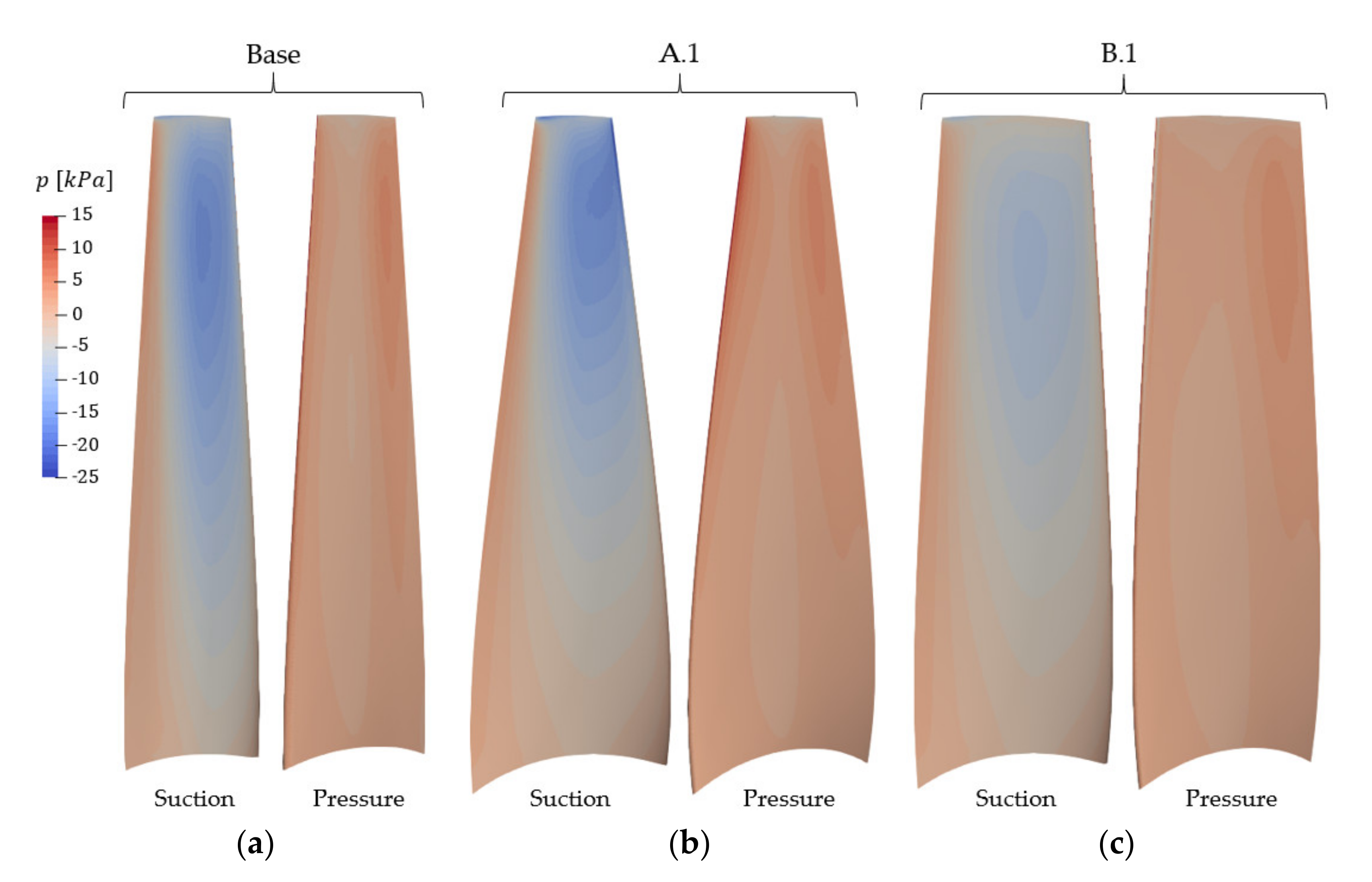
3.2. Optimization Results

Two alternative optimization problems were solved:
  • Problem A: Without imposing a constraint on the minimum pressure coefficient C p . M I N ;
  • Problem B: Imposing C p . M I N 3.5 (cavitation constraint).
The Pareto fronts for both cases, as well as the sample points used to generate the surrogate, are presented in Figure 6. The data point marked as “Base case” in Figure 6 represents the performance parameters of the initial geometry estimated using a RANS model. It can be seen that imposing a condition on the minimum pressure impacts the global maximum efficiency, as well as the maximum C P o w coefficient for a given thrust condition.
The base case was close to the Pareto front for unconstrained optimization, which shows that lifting line optimization methods were effective for the preliminary design stage. By exploring the Pareto front for Problem A, three different optimized solutions could be selected starting from the base case: A.1, the global maximum, A.2, which maximizes C P o w for a constant C T , and A.3, which minimizes C T for a constant C P o w . The global maximum for Problem B was identified as solution B.1. The design variables and response parameters for all solutions are listed in Table 2. The blade geometry for the base case and the optimized geometries A.1 and B.1 are presented in Figure 3.
The power coefficient for the base case was 0.428. The global maximum A.1 reached a power coefficient of 0.463, which represented an absolute increase of 3.5% and a relative increase of 8%. However, the thrust coefficient C T for A.1 was 0.860, which corresponded to an absolute increase of 15.3%.
Figure 7 compares the nondimensional chord c / D , the pitch angle ϕ , and the nondimensional maximum camber f m a x / c for the base geometry and optimized geometries A.1 and B.1. Figure 7d shows the nondimensional maximum thickness t m a x / D , which was kept constant for all geometries.
The pressure on both sides of the blade for the base case, the global maximum A.1, and the constrained optimization global maximum B.1 are compared in Figure 8. It is well-known that increasing the chord typically improves cavitation performance [12], which was reflected in the B.1 blade geometry obtained through automated optimization. Viscous losses, however, scale with the chord, so increasing the power output requires increasing the loading on the blade with respect to the base case.
RANS simulations can provide useful information on the characteristics of the HKT wake in order to optimize turbine location and the layout of turbine farm arrays [15]. The vorticity in the HKT wake can be visualized using the Q criterion, commonly used to study vorticity in wind turbine wakes [42]. Figure 9 shows the vortical structures in the wake for the initial geometry and the optimized geometries A.1 and B.1 as represented by the Q = 0.1 iso-surface. Optimized geometry A.1 showed increased wake vorticity and a greater expansion of the wake diameter, which is expected due to the higher thrust on the optimized blade. The wake for the B.1 case showed slightly higher vorticity than the base case.

4. Conclusions

In this article, we presented an optimization method which allowed for automated, systematic design of HKT rotor blades for all combinations of inflow and installation conditions.
The results prove the suitability of surrogate-based optimization to efficiently improve the power output of hydrokinetic turbines designed using simplified methods such as lifting line or BEM solvers, based on a limited number of analysis runs performed with a computationally expensive CFD solver. The optimization method allowed for the representation of arbitrary hub geometries and, if the periodic domain assumption was not adopted, could be extended to consider the influence of the support structure and nonsymmetric inflow conditions.
Two performance parameters were selected in the optimization algorithm: the power coefficient C P o w and the thrust coefficient C T . Maximizing C P o w while minimizing C T resulted in a series of optimal solutions forming a Pareto front. The final selection of an optimum turbine blade requires an economic analysis comparing the overall cost of the turbine, including its support structure, and the energy generated by the turbine.
The blade geometry design space depends on the starting geometry and the selected design variables. Furthermore, different assumptions for blade sectional properties will generate different blade geometry families. Future research will focus on the use of blade profiles designed for their use in HKTs, which prioritize high lift-to-drag ratios, reduced sensitivity to biofouling, good stall characteristics, and low susceptibility to cavitation and singing [2]. Better estimates for maximum thickness distributions will require the use of structural analysis tools.

Author Contributions

Conceptualization, D.M.A.; methodology, D.M.A.; software, D.M.A.; writing—original draft preparation, D.M.A.; writing—review and editing, Á.M.; supervision, Á.M. All authors have read and agreed to the published version of the manuscript.

Funding

This research received no external funding.

Acknowledgments

The computational resources used in this work were provided in part by the HPC centers DIRAC, funded by Instituto de Física de Buenos Aires (UBA-CONICET) and part of SNCAD-MinCyT initiative, Argentina, and TUPAC, funded by CSC-CONICET. The authors are also grateful for the support provided by Damwatch Engineering Limited.

Conflicts of Interest

The authors declare no conflict of interests.

References

  1. Laws, N.D.; Epps, B.P. Hydrokinetic energy conversion: Technology, research, and outlook. Renew. Sustain. Energy Rev. 2016, 57, 1245–1259. [Google Scholar] [CrossRef] [Green Version]
  2. Shiu, H.; van Dam, C.P.; Johnson, E.; Barone, M.; Phillips, R.; Straka, W.; Fontaine, A.; Jonson, M. A Design of a Hydrofoil Family for Current-Driven Marine-Hydrokinetic Turbines. In Proceedings of the 2012 20th International Conference on Nuclear Engineering and the ASME 2012 Power Conference, Anaheim, CA, USA, 30 July–3 August 2012; 2012. [Google Scholar] [CrossRef]
  3. Walker, J.M.; Flack, K.A.; Lust, E.E.; Schultz, M.P.; Luznik, L. Experimental and numerical studies of blade roughness and fouling on marine current turbine performance. Renew. Energy 2014, 66, 257–267. [Google Scholar] [CrossRef]
  4. Hansen, M.O.L. Aerodynamics of Wind Turbines, 3rd ed.; Routledge: London, UK, 2015. [Google Scholar] [CrossRef]
  5. Vogel, C.R.; Willden, R.H.J.; Houlsby, G.T. Blade element momentum theory for a tidal turbine. Ocean Eng. 2018, 169, 215–226. [Google Scholar] [CrossRef]
  6. Togneri, M.; Pinon, G.; Carlier, C.; Bex, C.C.; Masters, I. Comparison of synthetic turbulence approaches for blade element momentum theory prediction of tidal turbine performance and loads. Renew. Energy 2020, 145, 408–418. [Google Scholar] [CrossRef]
  7. Kerwin, J.E.; Hadler, J.B. Propulsion; Society of Naval Architects and Marine Engineers: Jersey City, NJ, USA, 2010. [Google Scholar]
  8. Epps, B.P.; Kimball, R. Unified Rotor Lifting Line Theory. J. Ship Res. 2013, 57, 181–201. [Google Scholar] [CrossRef]
  9. Menéndez Arán, D.H.; Tian, Y.; Kinnas, S.A. Effect of wake alignment on turbine blade loading distribution and power coefficient. J. Offshore Mech. Arct. Eng. 2019, 141, 041901. [Google Scholar] [CrossRef]
  10. Falcão de Campos, J.A.C. Hydrodynamic Power Optimization of a Horizontal Axis Marine Current Turbine With Lifting Line Theory. In Proceedings of the 17th International Offshore and Polar Engineering Conference, Lisbon, Portugal, 1–6 July 2007. [Google Scholar]
  11. He, L.; Kinnas, S.A.; Xu, W. A Vortex-Lattice Method for the Prediction of Unsteady Performance of Marine Propellers and Current Turbines. Int. J. Offshore Polar Eng. 2013, 23, 210–217. [Google Scholar]
  12. Xu, W. Numerical Techniques for the Design and Prediction of Performance of Marine Turbines and Propellers. Master of Science Thesis, The University of Texas at Austin, Austin, TX, USA, 2010. [Google Scholar]
  13. Baltazar, J.; Falcão de Campos, J.A.C. Hydrodynamic Analysis of a Horizontal Axis Marine Current Turbine With a Boundary Element Method. J. Offshore Mech. Arct. Eng. 2011, 133, 041304. [Google Scholar] [CrossRef]
  14. Salvatore, F.; Sarichloo, Z.; Calcagni, D. Marine Turbine Hydrodynamics by a Boundary Element Method with Viscous Flow Correction. J. Mar. Sci. Eng. 2018, 6, 53. [Google Scholar] [CrossRef] [Green Version]
  15. Yang, X.; Khosronejad, A.; Sotiropoulos, F. Large-eddy simulation of a hydrokinetic turbine mounted on an erodible bed. Renew. Energy 2017, 113, 1419–1433. [Google Scholar] [CrossRef]
  16. Sanderse, B.; van der Pijl, S.P.; Koren, B. Review of computational fluid dynamics for wind turbine wake aerodynamics. Wind Energ. 2011, 14, 799–819. [Google Scholar] [CrossRef] [Green Version]
  17. Lynch, C.E. Advanced CFD Methods for Wind Turbine Analysis. Ph.D. Thesis, Georgia Institute of Technology, Atlanta, GA, USA, 2011. [Google Scholar]
  18. Lawson, M.J.; Li, Y.; Sale, D.C. Development and Verification of a Computational Fluid Dynamics Model of a Horizontal-Axis Tidal Current Turbine. In Proceedings of the ASME 2011 30th International Conference on Ocean, Offshore and Arctic Engineering, Rotterdam, The Netherlands, 19–24 June 2011. [Google Scholar] [CrossRef] [Green Version]
  19. Lee, J.H.; Park, S.; Kim, D.H.; Rhee, S.H.; Kim, M. Computational methods for performance analysis of horizontal axis tidal stream turbines. Appl. Energy 2012, 98, 512–523. [Google Scholar] [CrossRef]
  20. Mukherji, S.S.; Kolekar, N.; Banerjee, A.; Mishra, R. Numerical investigation and evaluation of optimum hydrodynamic performance of a horizontal axis hydrokinetic turbine. J. Renew. Sustain. Energy. 2011, 3, 063105. [Google Scholar] [CrossRef] [Green Version]
  21. OpenFOAM Web Page. Available online: http://openfoam.com (accessed on 1 June 2021).
  22. Forrester, A.; Sobester, A.; Keane, A. Engineering Design via Surrogate Modelling: A Practical Guide; John Wiley & Sons, Ltd.: Hoboken, NJ, USA, 2008. [Google Scholar] [CrossRef]
  23. Dakota Web Page. Available online: https://dakota.sandia.gov (accessed on 1 June 2021).
  24. Thelen, A.S. Surrogate-based design optimization of dual-rotor wind turbines using steady RANS equations. Master of Science Thesis, Iowa State University, Ames, IA, USA, 2016. [Google Scholar] [CrossRef]
  25. Kumar, M.; Nam, G.W.; Oh, S.J.; Seo, J.; Samad, A.; Rhee, S.H. Design optimization of a horizontal axis tidal stream turbine blade using CFD. In Proceedings of the 5th International Symposium on Marine Propulsors, Espoo, Finland, 12–15 June 2017. [Google Scholar]
  26. Pholdee, N.; Bureerat, S.; Nuantong, W. Kriging Surrogate-Based Genetic Algorithm Optimization for Blade Design of a Horizontal Axis Wind Turbine. Comput. Model Eng. Sci. 2021, 126, 261–273. [Google Scholar] [CrossRef]
  27. Karthikeyan, T.; Avital, E.J.; Venkatesan, N.; Samad, A. Optimization of a horizontal axis marine current turbine via surrogate models. Ocean Syst. Eng. 2019, 9, 111–133. [Google Scholar] [CrossRef]
  28. OpenProp Web Page. Available online: https://engineering.dartmouth.edu/openprop/ (accessed on 1 June 2021).
  29. Moreu, J.; Epps, B.P.; Valle, J.; Taboada, M.; Bueno, P. Variational optimization of hydrokinetic turbines and propellers operating in a non-uniform flow field. Ocean Eng. 2017, 135, 207–220. [Google Scholar] [CrossRef]
  30. Kinnas, S.; Xu, W.; Yu, Y.H.; Lei, H. Computational methods for the design and prediction of performance of tidal turbines. J. Offshore Mech. Arct. Eng. 2012, 134, 011101-1. [Google Scholar] [CrossRef]
  31. Melo, D.B.; Baltazar, J.; Falcão de Campos, J.A.C. A numerical wake alignment method for horizontal axis wind turbines with the lifting line theory. J. Wind. Eng. Ind. Aerodyn. 2018, 174, 382–390. [Google Scholar] [CrossRef]
  32. Abbott, I.H.; von Doenhoff, A.E. Theory of Wing Sections; Dover Publications: New York, NY, USA, 1959. [Google Scholar]
  33. Weller, H.G.; Tabor, G.; Jasak, H.; Fureby, C. A tensorial approach to computational continuum mechanics using object-oriented techniques. Comput. Phys. 1998, 12, 620–631. [Google Scholar] [CrossRef]
  34. Menter, F.R. Two-Equation Eddy-Viscosity Turbulence Models for Engineering Applications. AIAA J. 1994, 32, 269–289. [Google Scholar] [CrossRef] [Green Version]
  35. Roache, P.J. Verification and Validation in Computational Science and Engineering; Hermosa: Albuquerque, NM, USA, 1998. [Google Scholar]
  36. Wang, D.; Atlar, M.; Sampson, R. An experimental investigation on cavitation, noise, and slipstream characteristics of ocean stream turbines. In Proceedings of the Institution of Mechanical Engineers, Part A. J. Power Energy 2007, 221, 219–231. [Google Scholar] [CrossRef]
  37. Díaz-Manríquez, A.; Toscano-Pulido, G.; Gómez-Flores, W. On the selection of surrogate models in evolutionary optimization algorithms. In Proceedings of the 2011 IEEE Congress of Evolutionary Computation (CEC), New Orleans, LA, USA, 5–8 June 2011; pp. 2155–2162. [Google Scholar] [CrossRef]
  38. Giunta, A.A.; Swiler, L.P.; Brown, S.L.; Eldred, M.S.; Richards, M.D.; Cyr, E.C. The Surfpack Software Library for Surrogate Modeling of Sparse Irregularly Spaced Multidimensional Data. In Proceedings of the 11th AIAA/ISSMO Multidisciplinary Analysis and Optimization Conference, Portsmouth, VA, USA, 6–8 September 2006. AIAA Paper 2006-7049. [Google Scholar] [CrossRef] [Green Version]
  39. Adams, B.M.; Bohnhoff, W.J.; Dalbey, K.R.; Ebeida, M.S.; Eddy, J.P.; Eldred, M.S.; Hooper, R.W.; Hough, P.D.; Hu, K.T.; Jakeman, J.D.; et al. A Multilevel Parallel Object-Oriented Framework for Design Optimization, Parameter Estimation, Uncertainty Quantification, and Sensitivity Analysis: Version 6.13 User’s Manual; Sandia Technical Report SAND2020-12495; Sandia National Laboratories,: Albuquerque, NM, USA, 2020. [Google Scholar]
  40. Guerrero, J.; Cominetti, A.; Pralits, J.; Villa, D. Surrogate-Based Optimization Using an Open-Source Framework: The Bulbous Bow Shape Optimization Case. Math. Comput. Appl. 2018, 23, 60. [Google Scholar] [CrossRef] [Green Version]
  41. Guerrero, J.; Mantelli, L.; Naqvi, S.B. Cloud-Based CAD Parametrization for Design Space Exploration and Design Optimization in Numerical Simulations. Fluids 2020, 5, 36. [Google Scholar] [CrossRef] [Green Version]
  42. Aseyev, A.S.; Cal, R.B. Vortex identification in the wake of a model wind turbine array. J. Turbul. 2015, 17, 357–378. [Google Scholar] [CrossRef]
Figure 1. CFD model domain and boundary conditions.
Energies 14 04045 g001
Figure 2. Typical medium mesh used for the RANS analysis simulations: (a) Longitudinal section along x z plane y = 0 ; (b) detail of longitudinal section on turbine area; (c) detail of surface mesh at blade root.
Energies 14 04045 g002
Figure 3. Cross sections and 3D blade geometry: (a) Initial geometry; (b) optimized geometry A.1; (c) optimized geometry B.1.
Energies 14 04045 g003
Figure 4. Optimization workflow.
Energies 14 04045 g004
Figure 5. Scatter plot matrix for the data used to build the surrogate model.
Energies 14 04045 g005
Figure 6. Pareto fronts for both optimization cases, with and without a constraint on C p . M I N .
Energies 14 04045 g006
Figure 7. Blade geometry for base and optimized cases: (a) c / D ; (b) ϕ ; (c) f m a x / c ; (d) t m a x / D .
Energies 14 04045 g007
Figure 8. Pressures distribution on blade suction and pressure sides: (a) Initial geometry; (b) optimized geometry A.1; (c) optimized geometry B.1.
Energies 14 04045 g008
Figure 9. Vortical structures in HKT wake as identified by the Q-criterion (iso-surface Q = 0.1): (a) Initial geometry; (b) optimized geometry A.1; (c) optimized geometry B.1.
Energies 14 04045 g009aEnergies 14 04045 g009b
Table 1. Convergence analysis results for C P o w .
kMeshNumber of Cells Average   y + C P o w = ϕ k GCI i Δ C P o w
1Coarse1.9M~130.423
2Medium3.6M~80.4280.0120.005
3Fine7.2M~40.4300.0040.002
Table 2. Optimization results.
Case a 1 a 2 b 1 b 2 c 1 c 2 C P o w C T C p . M I N
Base1111110.4280.7075.756
A.11.5210.9841.2580.5320.5271.0200.4630.8608.903
A.21.9780.5821.2580.8480.5070.7800.4370.7057.916
A.31.9800.6201.6040.8990.8960.9960.4270.6866.241
B.11.3711.8181.1721.0720.5670.8080.4370.7423.407
Publisher’s Note: MDPI stays neutral with regard to jurisdictional claims in published maps and institutional affiliations.

