1. Introduction
The impact of COVID-19 cannot be compared to any previous global crisis because the challenges of the current pandemic are much greater than during previous events. This is mainly due to the fact that we live in a much more globalised world. The current pandemic has considerable potential to devastate the economy. The result is a slowdown in economic development or even recession. The introduction of various types of lockdowns and the fear of the effects of the disease encompassing the whole of society lead to an amplification of its negative effects [
1]. This should therefore be managed effectively [
2,
3].
Energy risk has always been one of the main risk factors for most companies involved in key industrial sectors, both in developed and developing countries. Energy commodity risk management is a key issue for most industrial companies, as it can seriously affect their competitiveness and future profitability. Global economic developments, emerging technological advances, and economic, geopolitical, and environmental events have caused a significant increase in the volatility of energy commodity prices over the past 20 years [
4]. One such event is the COVID-19 pandemic. The negative effects of the pandemic, which were first felt in China and, from 2020 onwards, have spread worldwide. China accounts for a significant share of global commodity imports, which has had a knock-on effect on the entire international commodity market, and this may in turn affect economic growth [
5,
6,
7]. Negative effects include disruptions in global supply and demand chains and thus disruptions in the supply of goods. While the economic impact of the epidemic is multifaceted, this article assesses the connections between the increasing incidence and the energy sector. Commodity prices around the world have fallen significantly since the coronavirus outbreak. This may be attributed to the fall in demand in China, where manufacturing, air travel, and transport fuels have been severely affected [
8]. The global supply chain and financial system have been disrupted. In particular, lockdowns and the halting of international travel have reduced fuel consumption and consequently caused a lack of demand for oil [
9]. Commodity prices reacted strongly to the COVID-19 crisis, showing significant daily and weekly declines since February 2020. Price volatility across all types of commodities has also increased. In particular, the ups and downs of oil prices in March and April 2020 exceeded the fluctuations experienced during the global financial crisis of 2008–2009. In addition, the volatility of metal and agricultural commodity prices clearly exceeded the levels of recent years [
10]. Unconventional policy decisions by national governments can be more dangerous than the pandemic itself.
According to the World Bank [
11], the primary spill-over effects affecting commodity prices depend on the type of commodity. At the outbreak of the COVID-19 pandemic [
12]:
- (i)
the monthly price of crude oil plunged by almost 50% to a historic low, and some benchmarks recorded negative levels,
- (ii)
metal prices fell, with the most significant declines in zinc and copper, directly related to the slowdown in global economic activity,
- (iii)
agricultural commodity prices, which are less related to economic growth, have not declined significantly, with the exception of rubber, which is directly related to transport activities.
Already in the early stages of the pandemic, the energy sector was affected by COVID-19. This was mainly due to demand shocks. The decline in oil prices was due to the fall in demand. This also contributed to a decline in production. This was particularly evident in countries with price competition between the Organisation of the Petroleum Exporting Countries (OPEC) and Russia. The outbreak of the pandemic also had a negative impact on the nonenergy commodities sector. Many authors highlight the linkages between commodities, which may change during crises [
13,
14,
15,
16]. The link between energy and nonenergy commodities is most often analysed. Hence, the idea was born to investigate the linkage between energy commodities. The applied DTW method makes it possible to examine the similarities between the energy commodity price series and the series describing the number of cases.
It is still unclear when and how the COVID-19 outbreak will be brought under control. Therefore, it remains one of the important questions to be addressed to determine to what extent the outbreak has affected commodity prices so far. As the data and literature on the impact of the COVID-19 pandemic are still developing, definitive conclusions probably need to wait until the end of the pandemic.
It is expected that the COVID-19 pandemic will have a lasting impact on the consumption of energy resources, especially oil. During the epidemic, projections for oil demand have been revised as being down by major forecasters. They claim that the pandemic could have an impact on oil consumption by changing consumer behaviour. Air travel may be permanently reduced as business travel is restricted in favour of remote meetings, which reduces the demand for jet fuel. Working from home could reduce gasoline demand, but this may be offset by increased use of private vehicles if people refuse to use public transport.
Certainly, the pandemic has so far had a big impact on energy prices. The collapse in oil consumption in March and April 2020 resulted in a sharp decline in oil prices. In response, many oil producers cut production, in particular the Organization of the Petroleum Exporting Countries (OPEC) and its partners. As a result, the prices rebounded at a record pace from lows reached during the first phase of the pandemic. In the meantime, demand is also gradually increasing and is expected to stabilise in 2021 as vaccines become widely available and travel restrictions are eliminated.
The main purpose of our paper is the assessment of the similarity between the time series of energy commodity prices and the time series of daily COVID-19 cases using the dynamic time warping (DTW) method. We use the DTW measure to group energy commodities according to their price evolution and analyse the time shifts between daily COVID-19 cases and commodities prices. We conduct the analysis by subperiods in accordance with the timeline of the COVID-19 pandemic.
We find this motivation important, because direct relationships between the COVID-19 cases (or the phenomena that directly result from them) have already been widely analysed. In our research, we do not look for the direct impact of the COVID-19 cases on the energy commodity prices but rather the similarity in their courses. We also try to answer the question, if we can expect the changes in energy commodity prices on the basis of the evolution of the new COVID-19 cases (and find the time lag, after which we can expect the reaction of the prices to the changes of COVID-19 cases).
We put forward the following research hypotheses:
Hypothesis 1 (H1). The evolution of energy commodity prices is the result of the evolution of daily COVID-19 cases.
Hypothesis 2 (H2). The reaction of the energy commodity prices to daily COVID-19 cases is diverse with respect to their type.
We organise the manuscript as follows: in
Section 2 (Literature Review), we present the current research in the field of relationships between the spread of the COVID-19 pandemic on various aspects of the global economy, including the prices of energy commodities. In
Section 3 (Materials and Methods), we describe the data used in the research and applied research methodology: the Dynamic Time Warping (DTW) method and hierarchical clustering. In
Section 4 (Results and Discussion), we present the obtained results and discuss them in light of previous studies in this field. In the last section (Conclusions), we give the findings and present directions for future research.
2. Literature Review
Since the beginning of the pandemic, studies have been initiated worldwide on its impact on the economies of individual countries and on the global economy. As the pandemic continues to evolve, so do the results of early studies. In the early stages of the pandemic, studies of its negative impact on global GDP began to emerge [
17,
18,
19,
20,
21]. The decline in countries’ GDP was very much reflected in financial performance on the global stock exchange [
22]. Due to the estimated losses and decline in stock markets, there was a need for major policy interventions, both fiscal and monetary, and economic assistance to protect human health, prevent economic losses, and safeguard the financial health of the stock market [
23]. According to the existing literature [
24,
25], COVID-19 is similar to other crisis periods and thus can trigger financial panics and drive governments’ economic policy adjustments [
26]. Zhang, Hu, and Ji [
27] find that possible unconventional policy interventions could be more dangerous than the pandemic itself. However, the impact on policy need not be negative. Apergis and Apergis [
28] investigate the effect of the COVID-19 and oil prices on the US partisan conflict. Their findings imply that political leaders aim low for partisan gains during stressful times. Along with the numerous socioeconomic problems, there have also been technical problems faced by energy companies. One of the important challenges during the pandemic period has been the effective management of the energy sector. Demand for energy decreased due to a partial shutdown of industrial activity and stagnation in the transport sector (aviation, public transport, and individual transport). Satellite images from the European Space Agency show a decrease in nitrogen dioxide (NO
2) levels in the lower atmosphere during the blockade period. This is particularly evident in the world’s major cities [
29].
A body of research has emerged in the literature related to the impact of COVID-19 on commodity prices, including energy commodities. Amongst them, there is a number of research on the impact of the pandemic on oil prices. Albulescu [
21,
30] shows that the initial daily number of reported cases of new COVID-19 infections had a marginal negative impact on oil prices in the long run. COVID-19 primarily affected financial market volatility and economic policy uncertainty, which in turn affected oil price dynamics and volatility. Devpura and Narayan [
31] show that COVID-19 incidence and deaths contributed to oil price volatility ranging from 8% to 22%. Ertuğrul, Güngör, and Soytaş [
32] analyse the impact of the COVID-19 outbreak on the volatility dynamics of the Turkish diesel market. The abnormally high volatility started after 11 March 2020, the day the first case of COVID-19 was announced in Turkey. Volatility peaked in mid-April 2020 due to restrictions imposed by the Turkish government. Initial diesel purchases were dictated by uncertainty, followed by a steady decline in consumption. In response to Turkey’s normalisation policy, volatility approached zero over time. Gil-Alana and Monge [
33] analyse the time series of WTI crude oil prices. They show that oil price shocks during the first pandemic period were transitory, although they will have long-lasting effects. Narayan [
34] in his study finds that the oil price is more influenced by negative news about oil prices than the number of COVID-19 cases. This dominant influence of news is particularly evident once a certain threshold of price volatility is exceeded.
Changes in energy commodity prices affect changes in other commodity prices. Ezeaku, Asongu, and Nnanna [
12] analyse the impact of oil supply and global demand shocks on commodity prices in metals and agricultural commodity markets in the context of the COVID-19 pandemic. This pandemic has already had a significant impact on the economies of most countries and on international financial and commodity markets. The real-time reactions of metal prices to the oil shock differed between precious metals (gold and silver) and other base metals (copper and aluminium). Gold and silver prices reacted negatively to the oil shock throughout the pandemic period studied. Copper reacted positively to the oil shock from day 0 to day 130 (end of May 2020), after which its reaction to the oil shock became negative during the remaining period. The aluminium price, on the other hand, reacted positively to the oil shock over the entire period. The estimated impact of oil shocks on the prices of selected agricultural commodities varied for each commodity. Maize and wheat prices reacted positively and significantly to oil shocks, while the reaction of soybean and paddy rice prices to oil shocks turned negative. Baffes, Kabundi, and Nagle [
35] argue that unlike the demand for agricultural commodities, a slowdown in economic activity strongly affects the demand for energy and metals due to its higher income elasticity. Research by Vu et al. [
36] indicates that different agricultural shocks can also affect the oil price differently. This is the case for maize used for ethanol production.
In the contemporary literature on the economic impact of the pandemic, there have been studies on the mining industry. Laing [
37] analyses the declines in commodity prices. The mining industry saw a dramatic drop in demand due to the suspension of most industrial and construction production. This reduction in demand resulted in drastic price falls for a number of metals and minerals in March and April 2020. These falls were most drastic in the case of aluminium and copper. This led, in effect, to a fall in the share prices of many large international mining companies. The situation showed great similarities with the crisis of 2008–2009. Whether the pandemic’s drops in the value of large mining companies will continue and whether they will lead to drops on the scale of the previous crisis depends on the duration of the lockdown and on economic and social conditions. However, a clear difference between COVID-19 and the 2008–2009 crisis is the case of the gold industry. Today, investors and entrepreneurs have even moved away from the supposed safe haven of gold, choosing instead to hoard currencies, such as the US dollar, needed to finance companies that have experienced unprecedented revenue declines.
In their paper, Lin and Su [
14] analyse the linkages between commodities. They point out that due to COVID-19, energy commodity prices, as well as the financial market as a whole, exhibit many strange phenomena, such as extremely high price volatility, negative oil prices, and rapidly increasing systemic risk [
38]. On 2 March 2020, the number of COVID-19 pneumonia infections in the United States crossed the double-digit mark and started to rise continuously. This time span exactly coincides with a sharp jump in the linkage index, indicating a strong impact of COVID-19 on the change in the prices of energy commodities and products. Prior to this moment, the total linkage index had always remained stable and showed only a few spikes and long-term trends. When a major economic event takes place, financial market analysts and investors pay attention to whether and how the strength and structure of the linkages between these commodities change. In March 2020, the total linkages between energy commodity markets experienced a sharp exponential increase. Such a change is similar to the situation in the 2008 financial crisis. However, the impact of COVID-19 appears to have lasted for only two months, and total linkages returned to average levels as early as May 2020. The authors find that the pandemic has a limited impact on pairwise linkages between energy commodities. From a structure perspective, only WTI and gasoline changed the direction of net linkages, while other commodities show only a change in intensity. This implies that the correlation structure of energy commodities is more or less stable even during the pandemic period. With the gradual containment of the spread of COVID-19, the energy market is slowly recovering. Although the price of energy commodities is still low, spill-over relationships between different markets are returning to prepandemic conditions.
As Tröster and Küblböck [
10] note, the global spread of COVID-19 poses a huge challenge for developing countries. In addition to the health and economic crisis, many of them faced additional problems related to their dependence on commodities. Commodity price movements reflect changes in supply and demand in commodity markets but are also largely driven by policy measures to contain the pandemic. The crisis has once again exposed the structural weaknesses of commodity-dependent developing countries.
Foglia and Angelini [
39] study the volatility linkages between oil price and clean energy sector firms (wind, solar, and technology) over the period 2011–2020 with the COVID-19 outbreak. The results indicated a significant change in both static and dynamic volatility linkages around the COVID-19 outbreak. WTI oil went from being a transmitter of volatility (before the pandemic outbreak) to a receiver of risk after the onset of the global COVID-19 pandemic. The recent pandemic intensified the spread of volatility, supporting financial contagion effects. The results of the study supported the hypothesis that dynamic linkages between oil and the clean energy sector peak during turbulent periods. The study shows that the cleantech sector has become important in optimal diversification strategies. The results obtained can be used in portfolio decisions and regulatory policymaking, especially in the current context of high uncertainty.
Nyga-Lukaszewska and Aruga [
40] study how the pandemic affects oil and gas prices. For this purpose, they use energy market reactions in the United States and Japan. In the study, they analyse data covering the so-called ‘first wave of the pandemic’. They show that there are differences in the energy market response between the two countries. A possible explanation for these results could be the differences in the development of the pandemic in the US and Japan, as well as the different role of the two countries in the energy markets. The number of COVID-19 cases in the USA during the initial phase of the pandemic was more than a hundred times higher than in Japan. Most US states enacted stricter regulations on staying indoors. These included fines and other penalties for violating lockdown laws. In Japan, the government did not enact such strict lockdown laws, and as a result, many people continued to commute to work by public transportation, even after the state of emergency was declared.
Chaudhary, Bakhshi, and Gupta [
41] analyse the impact of COVID-19 on returns and volatility of stock indices of 10 major countries based on the GDP. The study period covers the first six months of the pandemic. They note the inherent uncertainty in the market, in that it is difficult to predict the long-term economic impact of COVID-19. This difficulty is due to the lack of existence of a comparable historical benchmark on which such predictions should be based.
Czech and Wielechowski [
42] in their study evaluate the impact of COVID-19 on stock indices related to the alternative and conventional energy sector. The analysed indices decline as the government anti-COVID-19 policy becomes more stringent, but the relationship is statistically significant only in the high-volatility regime. The alternative energy sector, represented by the MSCI Global Alternative Energy Index, seems to be more resistant to COVID-19 than the conventional energy sector. This might imply that the novel coronavirus pandemic has not depreciated but emphasised the growing concern about climate change and environmental pollution. Research by Norouzi et al. [
43] has shown that conventional electricity sources are not flexible enough to cope with a crisis during the pandemic. Electricity from renewable sources is more reliable than fossil fuels due to its availability in most regions.
Habib et al. [
44] analyse asymmetric links between the COVID-19 outbreak, oil prices, and atmospheric CO
2 emissions. They use the unique Morlet’s wavelet method in the analysis. The results of their study show strong but diverse relationships between the variables studied. The results also show that COVID-19 influenced oil prices and contributed most to the reduction of CO
2 emissions. The authors also show a negative relationship between COVID-19 and CO
2 emissions.
Hassan and Riveros Gavilanes [
45] use daily data to model the dynamic impact of the COVID-19 pandemic on the stock indices of the first affected countries and on global commodity markets. The panel least squares Vector Auto-Regressive (VAR) estimation results confirm the negative short-term impact of the virus spread rate on the returns of the stock market indices. The virus spread rate is significant in explaining changes associated with platinum, silver, West Texas Intermediate (WTI), and Brent crude oil prices. The largest decline is observed in the case of the price of a barrel of oil, where an increase in the virus spread rate caused Brent and WTI crude oil prices to decline by 4.08% and 3.26%, respectively.
Shehzad et al. [
46] use the Exponential Generalized Autoregressive Conditional Heteroskedasticity (EGARCH) model to assess the impact of the COVID-19 crisis on Dow Jones and West Texas Intermediate (WTI) oil returns in relation to other crises. Their results indicate that COVID-19 and the accompanying lockdown negatively affect both rates of return and that the impact on oil prices is more significant than on the Dow Jones index. They show that COVID-19 negatively affects investors’ ability to determine optimal portfolios and thus the stability of financial and energy markets more than the global financial crisis of 2007–2009.
Ahmed et al. [
47] study the impact of COVID-19 on the Indian stock and commodity markets during the different phases of lockdown. They also compare the impact of COVID-19 on the Indian stock and commodity markets during the first and second waves of the COVID-19 spread. They apply the conventional Welch test, heteroskedastic independent
t-test, and the GMM multivariate analysis on the stock return, gold prices, and oil prices. They show that during different phases of the lockdown in India, COVID-19 has a negative and significant impact on oil prices and stock market performance. In contrast, with respect to gold prices, the impact is positive and significant. COVID-19 has a significant impact on the stock market performance of other South Asian countries. However, this impact is only for a short period and diminishes in the second wave of the COVID-19 spread.
Chien et al. [
48] investigate the time-frequency relationship (the time-frequency relationship) between the COVID-19 pandemic and oil and stock market volatility, geopolitical risk, and economic policy uncertainty in the US, Europe, and China. They use the coherence wavelet method and the wavelet-based Granger causality tests to analyse the data. The results indicate a dramatic fall in oil and equity prices as COVID-19 intensified, proving to be much stronger after 5 April 2020. The oil market shows low co-movement with the stock exchange, exchange rate, and gold markets.
Other global and local factors also influence the demand for and supply of energy commodities. Not all changes occurring in the energy market should be explained solely by the impact of COVID-19. There are many factors that exist independently of the emergence of the pandemic. The “oil price war” between Saudi Arabia and Russia also contribute to the decline and destabilisation of oil prices in the first half of 2020 [
49]. The crisis caused by COVID-19 reveals the structural weaknesses of commodity-dependent developing countries [
10,
50]. The negative relationship between commodity dependence and economic and social development is primarily related to deteriorating terms of trade and volatility in global commodity prices. Differences in the health of the energy sector in different regions of the world and countries should not only be viewed in terms of the spread of the virus. These differences are influenced by the fact whether a given country is only a consumer or a consumer and producer (exporter) of fuel and energy resources [
40].
From a consumer perspective, many factors influence the prices of energy carriers. The most important of these are: costs of production, political situation, economic factors, freak weather conditions, ecological factors, social factors, and currency markets [
51].
Our research goes in a different direction, hence, the proposal to detect similarities between commodity price developments and the number of COVID-19 cases, as well as similarities between the prices of individual commodities.
3. Materials and Methods
3.1. Overview of the Research Area
We base our research on the data coming from two sources. Data regarding daily COVID-19 cases come from
https://ourworldindata.org/covid-cases service (accessed on 19 April 2021). Prices of commodities come from the
https://stooq.com/ service (accessed on 19 April 2021). Data covered the period from 2 January 2020 until 15 March 2021. We analyse the prices of the following energy commodities:
Brent crude oil (USD/barrel),
CO2 allowances (Euro/tonne),
Heating oil (USD/gallon),
Palm oil (INR/10 kg),
ULSD (Ultra Low-Sulphur Diesel) (USD/gallon),
Coal (USD/tonne),
Natural gas (USD/mmbtu (mmbtu stands for millions of British thermal units (1 mmbtu ≈ 293 kWh))),
Gasoline (USD/gallon),
Ethanol (USD/gallon),
Uranium (USD/lb).
The analysed period included days when there were no quotations (weekends and holidays). Therefore, for such days we interpolate the quotations on the level of average calculated from the values from the last day before and the first day after the period without quotations. Moreover, in order to mitigate the impact of possible errors arising from such a procedure, we calculate a 7 day moving average. We also calculate the 7 day moving average for the COVID-19 daily cases, in order to mitigate the effects of under-reporting them during weekends or holidays and over-reporting in subsequent days. Therefore, we set the period under analysis to 5 January 2020–12 March 2021.
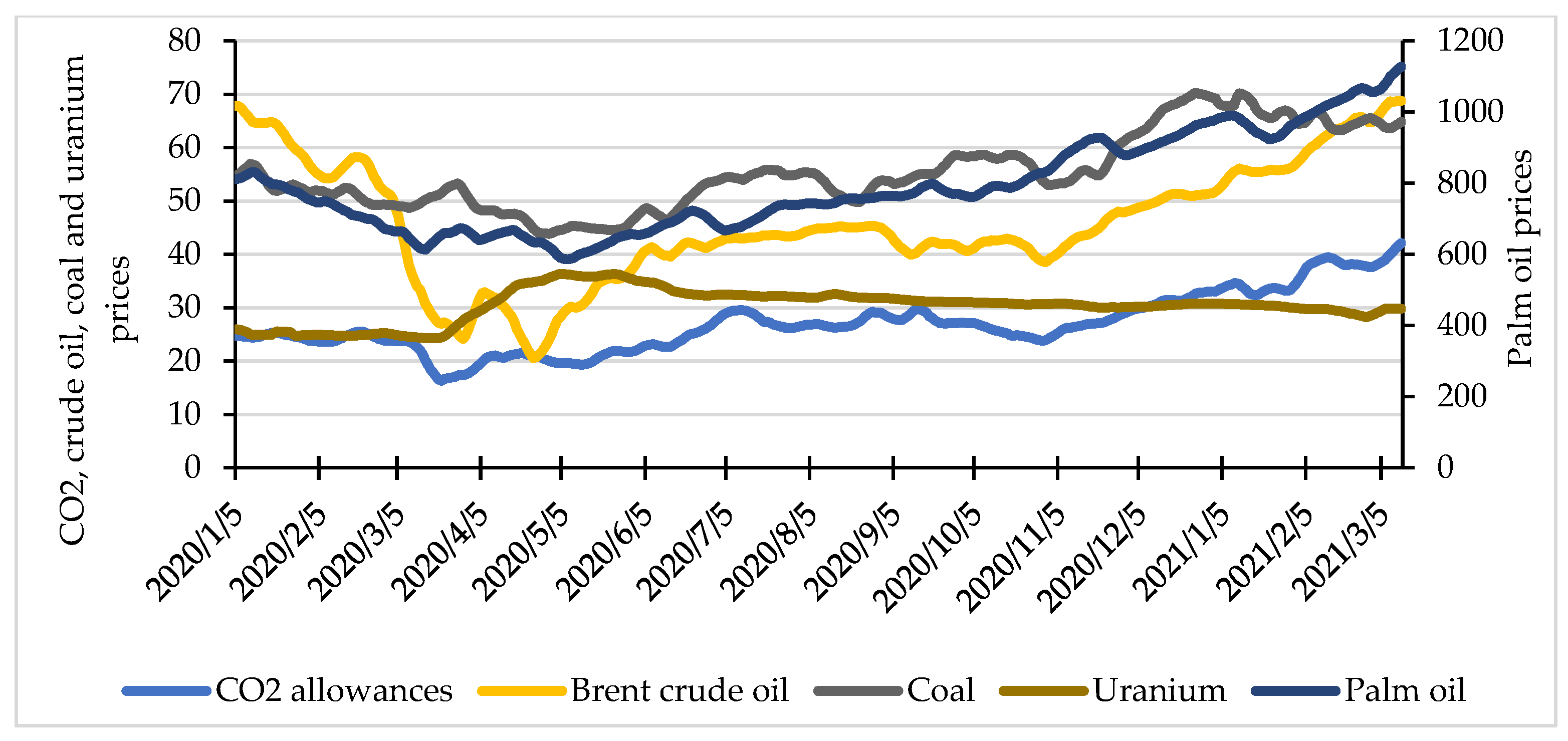
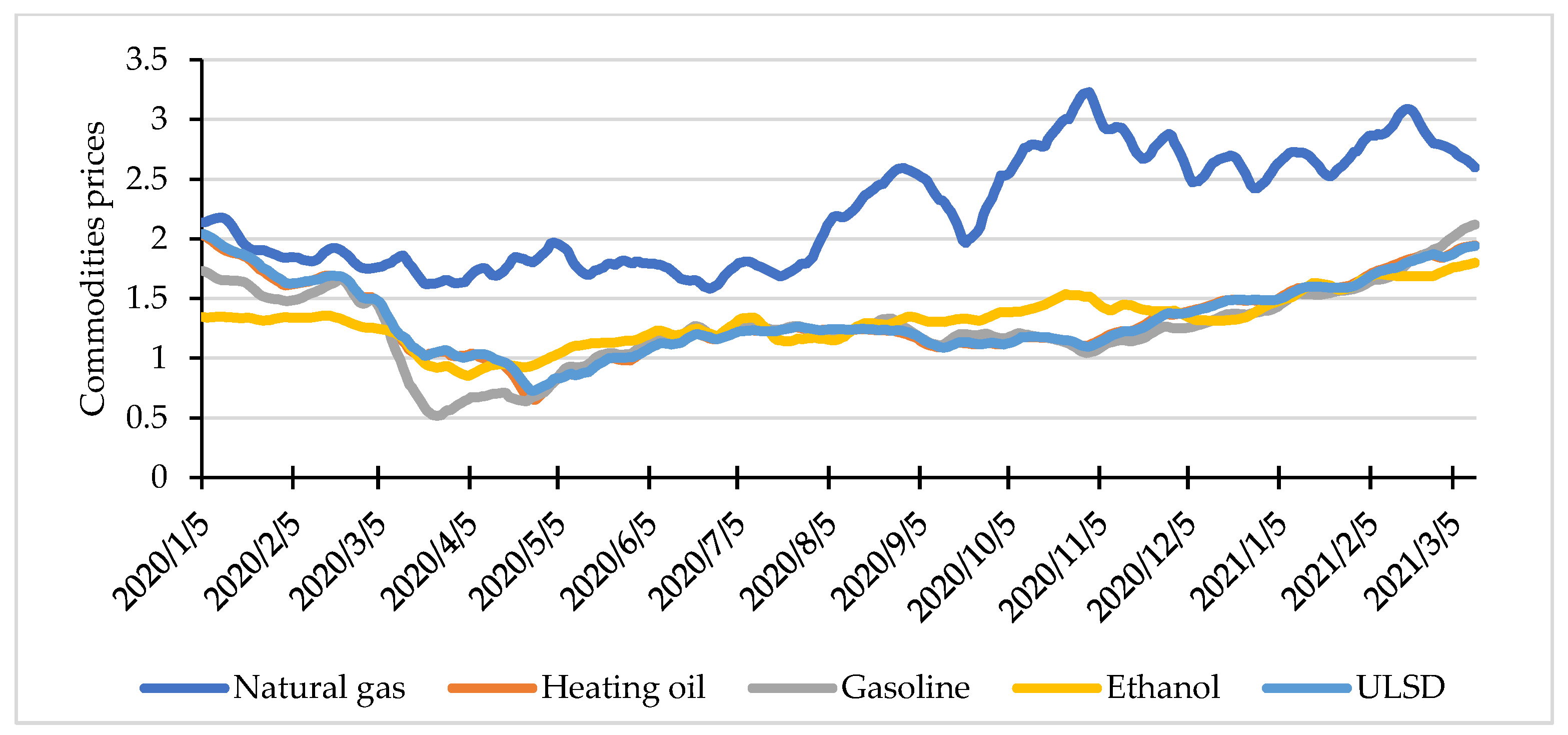
We present the courses of the process of analysed commodities in
Figure 1 and
Figure 2.
When analysing the course of prices of energy commodities, we can make several interesting observations. First, the uranium prices seem unrelated to the COVID-19 pandemic. The uranium price is generally more or less constant; only during the first wave of the pandemic (March 2020–beginning of May 2020) did it note an increase by about 40%. Since then, it was constantly, slowly decreasing until the end of the observation period.
We can make another interesting remark on the prices of heating oil, ULSD, and gasoline. Their courses are very similar to each other during the whole observation period. This was especially visible in the case of the pair ULSD—heating oil. It is perfectly understandable because these two fuels are essentially the same ones. A visible decrease in prices of these three commodities can be seen since the beginning of the pandemic, and it accelerated after the declaration of the pandemic by the World Health Organization (WHO)—11 March 2020. The decline of the gasoline decrease was deeper but ended earlier than for ULSD and heating oil, at the end of March 2020. Prices of heating oil and ULSD stopped falling at the end of April 2020. Since then, they gradually began to increase and continued this trend until the end of the observation period.
Ethanol prices noted a small decrease after the declaration of the state of pandemic, and since the beginning of April 2020, they were generally increasing with small fluctuations. Prices of natural gas showed no response to the first wave of the pandemic. After being at more or less the same level with fluctuations, it noted a big increase during August 2020 and remained on more or less the same level with big fluctuations afterward.
We observe a quite similar general course for the pair of coal–palm oil. Their prices were decreasing until the end of the first wave of the pandemic and started to grow afterward. The CO2 allowances prices noted a small decrease after the declaration of the pandemic state and were gradually increasing with fluctuations until the end of the observation period.
However, we observe the most interesting dynamics in the case of the crude oil price. It was decreasing since the beginning of the observation period, and the decline has been very sharp after the declaration of the pandemic state. After a significant increase after the first price depression (by 24%), it noted the second large drop until 25 April 2020 (by over 35%). It started to regain its value afterward and continued with fluctuations until the end of the observation period, when the price of crude oil reached virtually the same level as at the beginning.
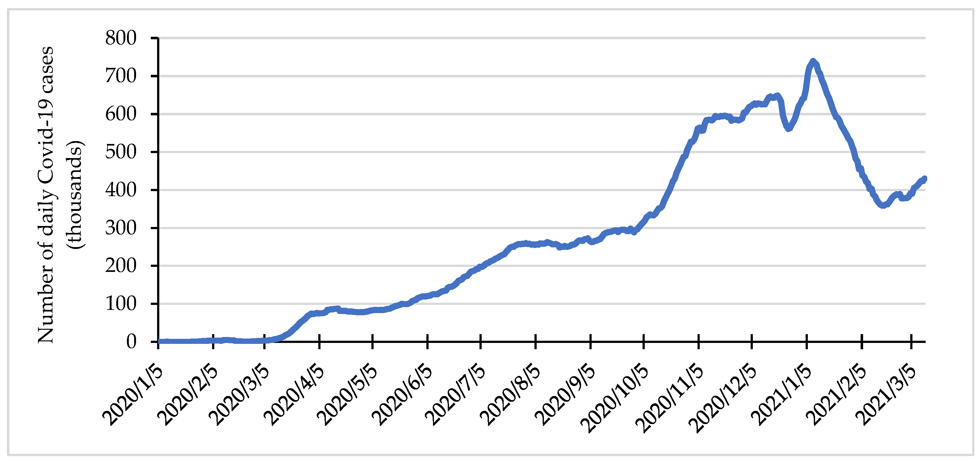
Since the beginning of the COVID-19 outbreak, the three waves have swept over the world. The first one took place during Spring 2020, the second one—in Autumn 2020—Winter 2020/2021, and the third one started at the end of February 2021 and is on an upward curve (as of mid-March 2021—
Figure 3). The first COVID-19 wave, as compared to the second one, was very shallow, but when we look at the prices of selected commodities (crude oil, gasoline, heating oil, ULDS, or ethanol), they reacted on this first wave much stronger than on the second one.
3.2. Research Methodology
To compare the time series for COVID-19 cases and for energy commodities prices, we use the Dynamic Time Warping (DTW) distance method. It calculates an optimal match between two given time series, performing nonlinearly in the series by stretching or compressing them locally in order to make one resemble the other as much as possible. This distortion (called warping) allows an adjustment of the time axis to find similar but phase-shifted sequences [
52].
The DTW method, invented by Bellman and Kalaba [
53], was originally developed for dealing with speech recognition problems [
54,
55,
56,
57]. It has been further used in a wide spectrum of different applications, e.g., in the field of music information retrieval [
58], for gesture recognition [
59], in bioinformatics [
60], in finance [
61], and for labour market analyses [
62].
The DTW is an algorithm for measuring similarity between two temporal sequences that utilises dynamic programming to find an optimal alignment between them with respect to a given scoring function.
Let
and
be two time series. In the first step, in order to make meaningful comparisons between two time series, both must be normalised. In the case of time series, a standard method of processing raw data is
z-normalisation. The need for time series normalisation is often emphasised in classification methods with the dynamic time warping and other distance measures [
63,
64].
In the next step, we define the local cost measure for two elements of
and
as:
Evaluating this measure for each pair of elements of X and , we obtain the local cost matrix (). Then, our goal is to find the optimal alignment between series and having minimal overall cost.
Such a point-to-point alignment between
and
can be represented by a time warping path, which is a sequence
, with
for
, satisfying the boundary, monotonicity, and step size conditions [
65]. The boundary condition ensures that the first and the last element of
are
and
(the first (last) index from the first sequence must be matched with the first (last) index from the other sequence). The other two conditions ensure that the path always moves up, right, or up and right of the current position, i.e.,
for
. Every index from the time series
must be matched with one or more indices from the time series
(and vice versa).
The optimal match is denoted by the match that satisfies all the abovementioned restrictions and that has the minimal total cost, where the total cost
of a warping path
is defined as:
The optimal match between
and
is then:
where
is the set of all possible warping paths.
The DTW algorithm finds the path that minimises the alignment between
and
by iteratively stepping through the local cost matrix and aggregating the cost. The optimal path
could be found using a dynamic programming algorithm, building the accumulated cost matrix
in the following way:
The DTW distance, i.e., the stretch-insensitive measure of the difference between the two time series, which is also the minimal distance between series and , is then defined as .
Once the accumulated cost matrix is constructed, the optimal warping path could be found by the simple backtracking from the top-right corner of this matrix (from the point ) and traversing to the bottom-left. The traversal path is identified based on the neighbour with minimum value.
The shapes of the warping curves provide information about the pairwise correspondences of time points. Graphically, the optimal warping path
runs along a “valley” of low cost and avoids “mountains” of high cost [
66]. If
is above diagonal, then the time series
leads
. It is also possible to determine by how many lags time series
leads time series
. For this purpose, we calculate the median value for the differences between the indices of
[
52]. Negative values indicate that the time series
leads time series
, positive that
leads
.
In our paper, the values of the DTW distance between the time series analysed are computed using the
dtw package (version 1.22-3) for R [
67].
The calculated distances have a straightforward application in hierarchical clustering and classification [
68]. Clustering is a technique in which similar data are divided into homogeneous groups. There are many clustering methods. They can be divided into homogeneous groups, optimising the initial division of objects. They are widely used in general and spatial economics research [
69,
70,
71,
72,
73,
74,
75,
76].
After measuring the similarities between the time series using DTW, we perform the agglomerative hierarchical clustering, mainly due to its great visualisation power. In this contribution, to carry out the hierarchical cluster tree, the average linkage with the squared Euclidean distance is used.
4. Results and Discussion
With accordance to the timeline of the COVID-19 pandemic, we perform the research in four periods:
the whole period (5 January 2020–12 March 2021),
first subperiod, covering data from the beginning until the peak of the first wave of the pandemic (27 April 2020).
second subperiod, covering data from the peak of the first wave until the peak of the second one (28 April 2020–7 January 2021).
third subperiod, covering data from the peak of the second wave (8 January 2021) onwards.
In the whole period and in every subperiod, we perform the analysis in the following steps:
We standardise all time series.
We calculate the DTW distance between the standardised COVID-19 time series and time series of all commodities.
We calculate the DTW distance matrix between all commodities.
On the basis of distance matrix calculated in point 3, we conduct the hierarchical clustering of commodities. We check the robustness of clustering by comparing obtained results with the results obtained by the k-medoids and divisive hierarchical clustering.
We analyse pairs of the best- and the worst-fitted time series.
We group the commodities with respect to their distance from the COVID-19 time series. We create the two groups—with distance smaller than median (denoted by A) and larger than median (denoted by B).
We identify the lags between the COVID-19 and commodities time series by determining the median differences between the optimal path indices.
After standardisation of all time series, the preliminary analysis showed that the course of the uranium prices was different than both COVID-19 cases and prices of commodities to such extent that it formed a separate cluster, with all other commodities being in the second one, both over the full period and in subperiods. Therefore, we decided to remove the uranium from further analysis.
4.1. Full Period
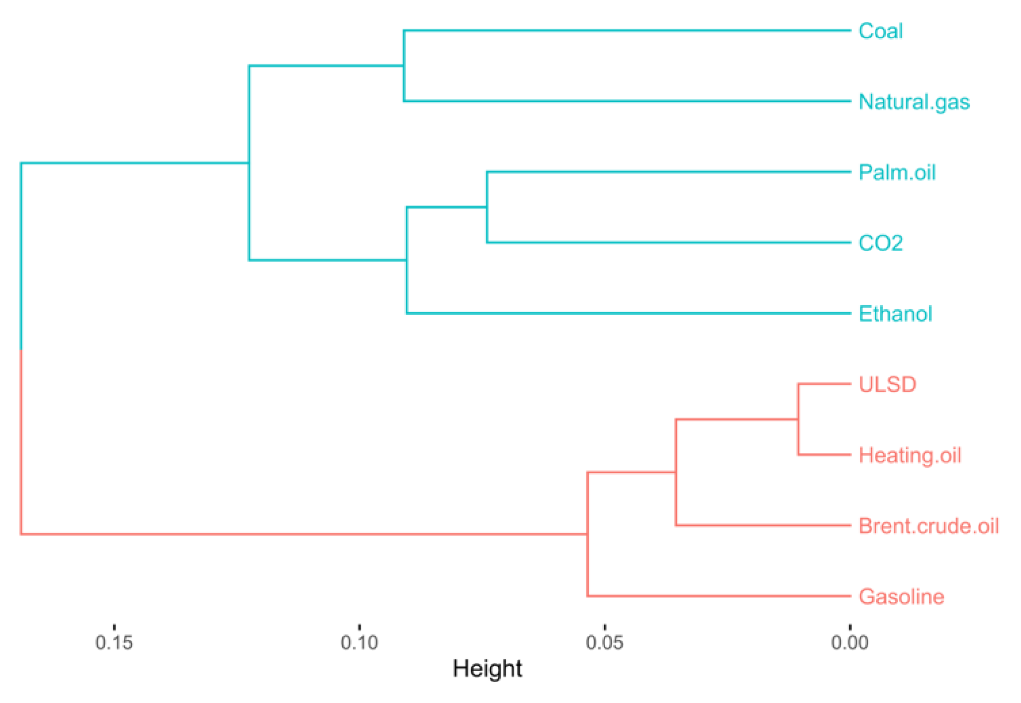
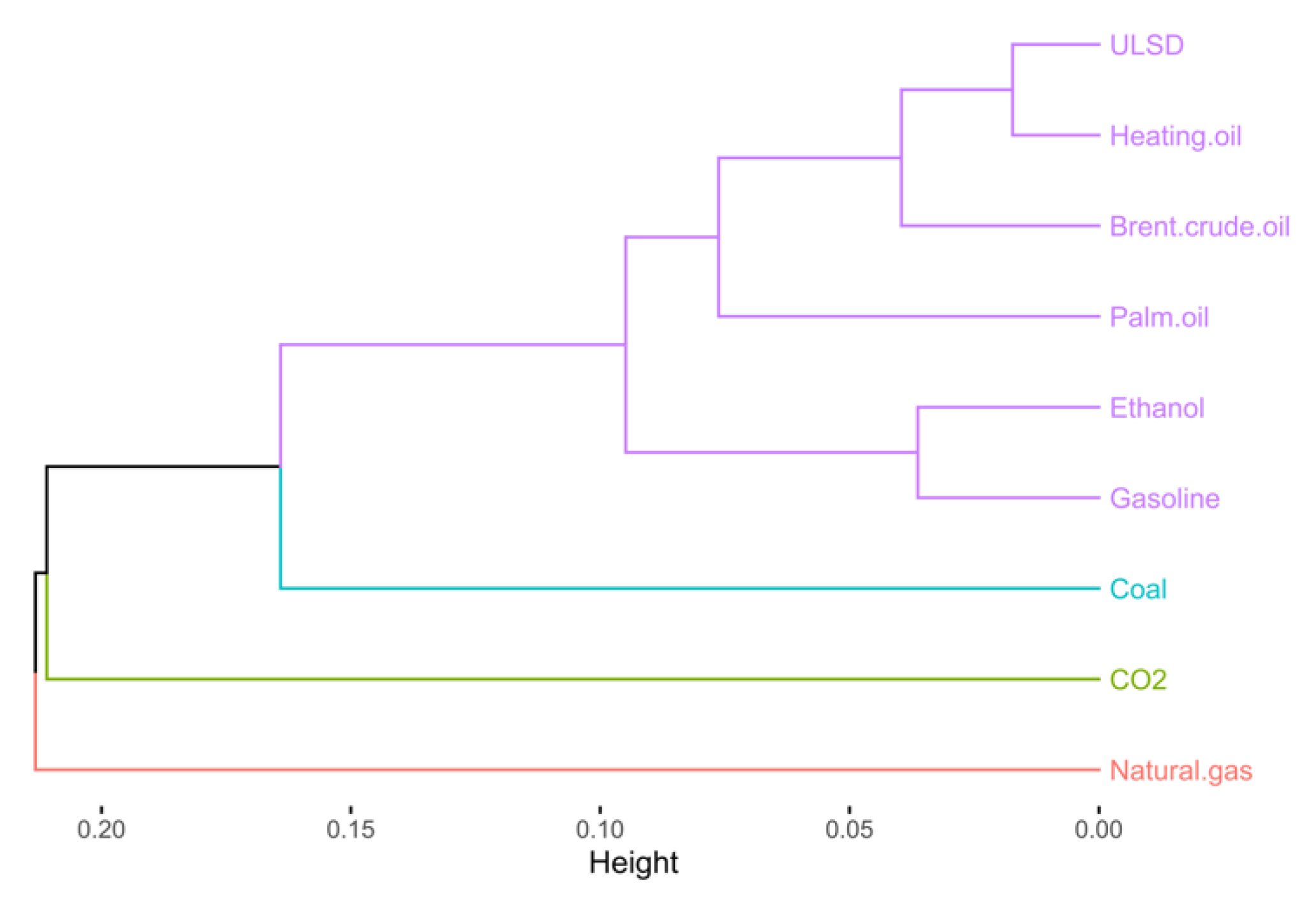
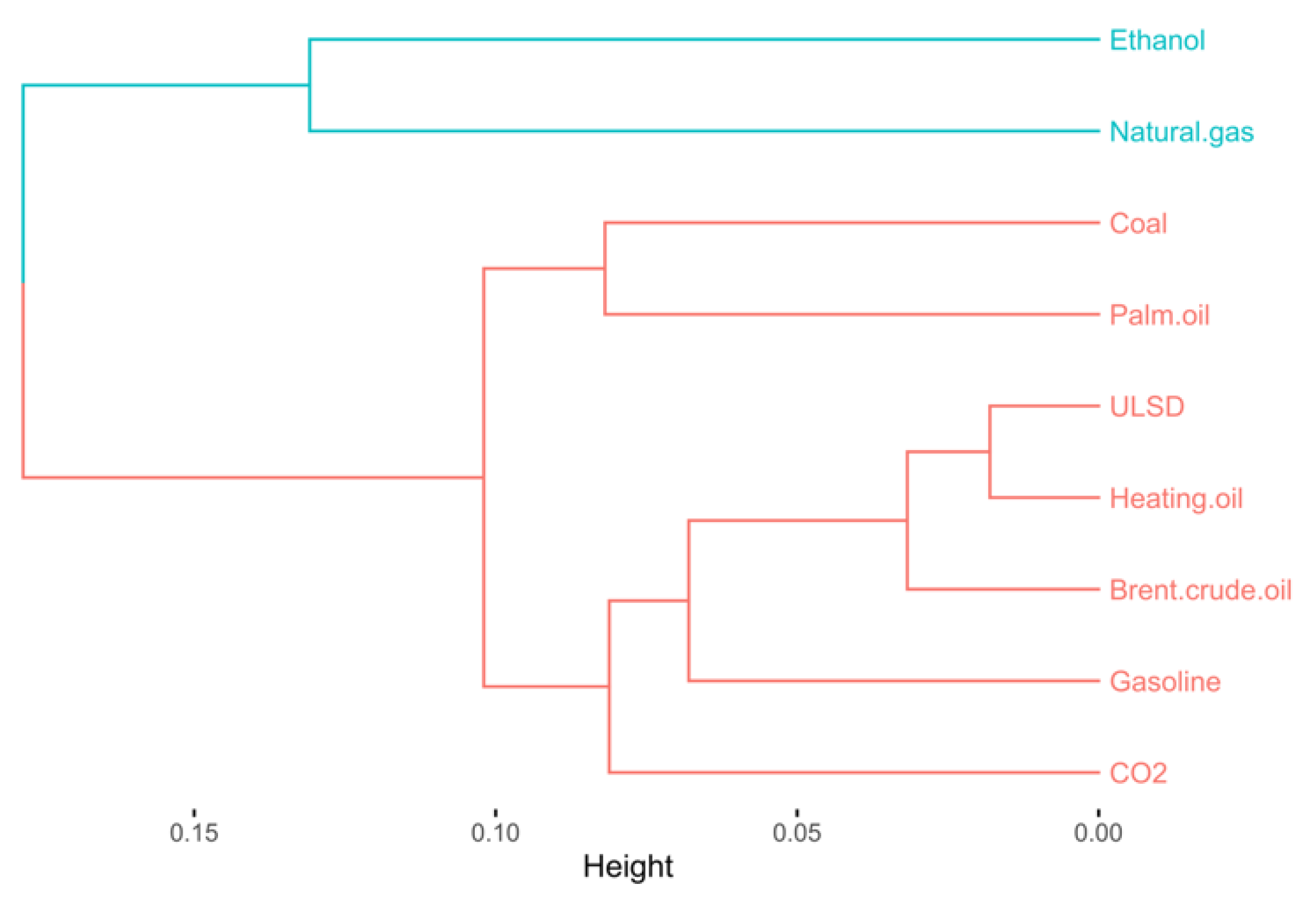
We present the dendrogram for the prices of analysed commodities in
Figure 4.
On the basis of the dendrogram, we distinguish two clusters of commodities, with ULSD, heating oil, crude oil, and gasoline forming the first one, which was much more homogenous than the second one (which is quite obvious, as the dynamics of prices of ULSD, heating oil, gasoline and Brent oil are very similar—
Figure 1 and
Figure 2. We obtain the same results for the
k-medoids and divisive hierarchical clustering methods.
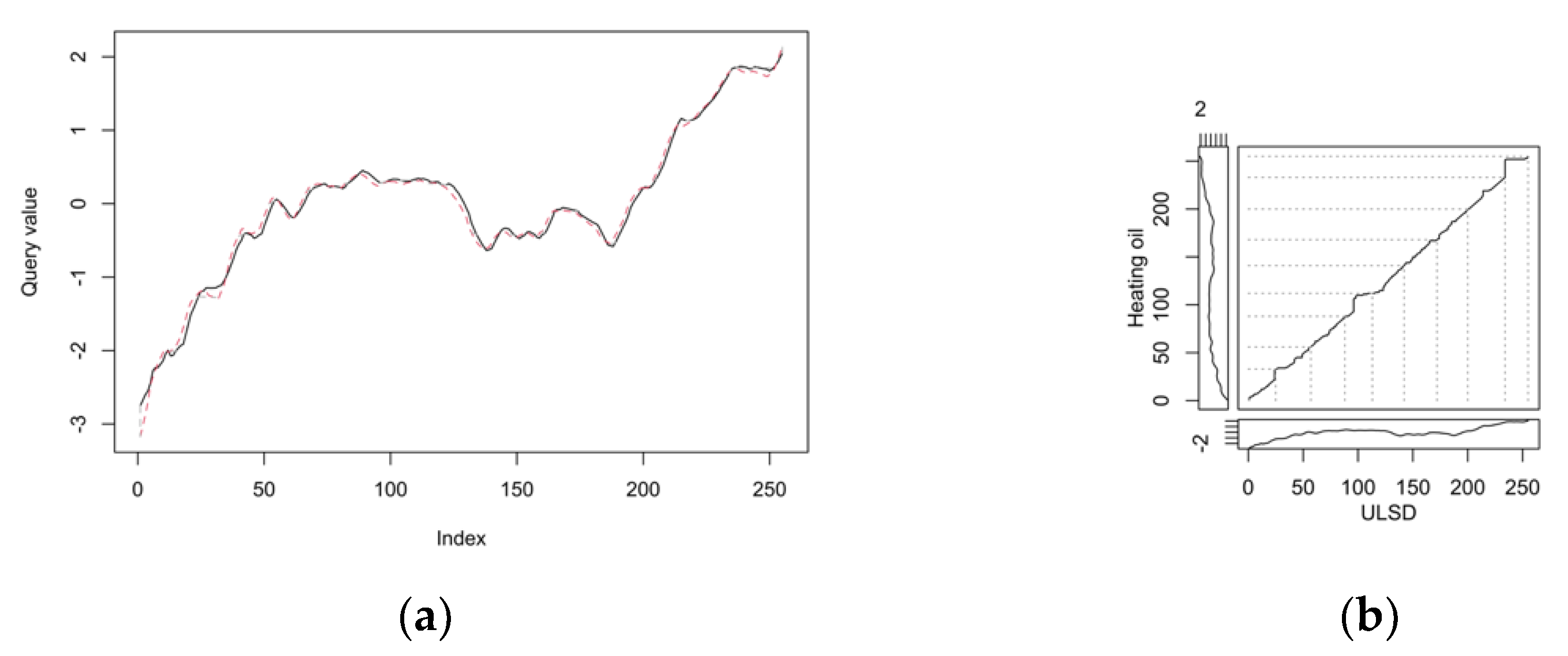
The two most similar commodities with respect to time-series courses are ULSD and heating oil. The DTW distance for them is the smallest and equals 0.011. We present here two-way and three-way alignment plots in
Figure 5.
Both charts indicate that the courses of ULSD and heating oil are virtually identical—two-way plots are practically overlapping, and the three-way plot goes through the minor diagonal. In addition, from the two-way alignment plot, we can judge about the differences between indices—there is virtually no difference (the price of heating oil is just one day ahead of ULSD price).
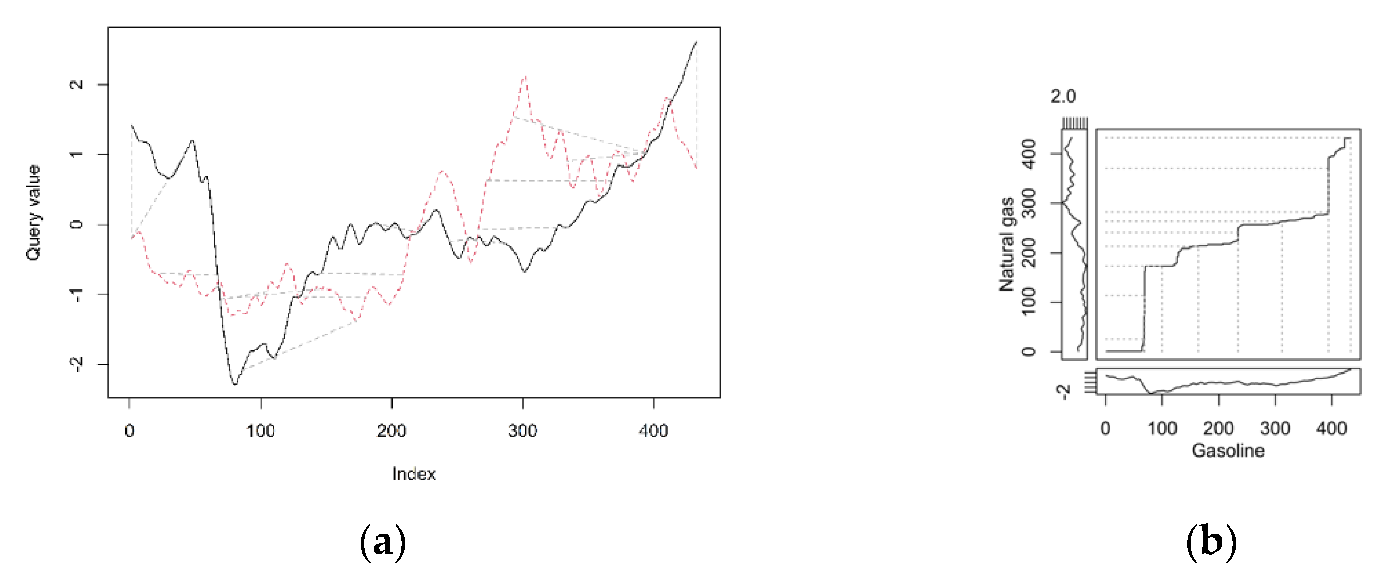
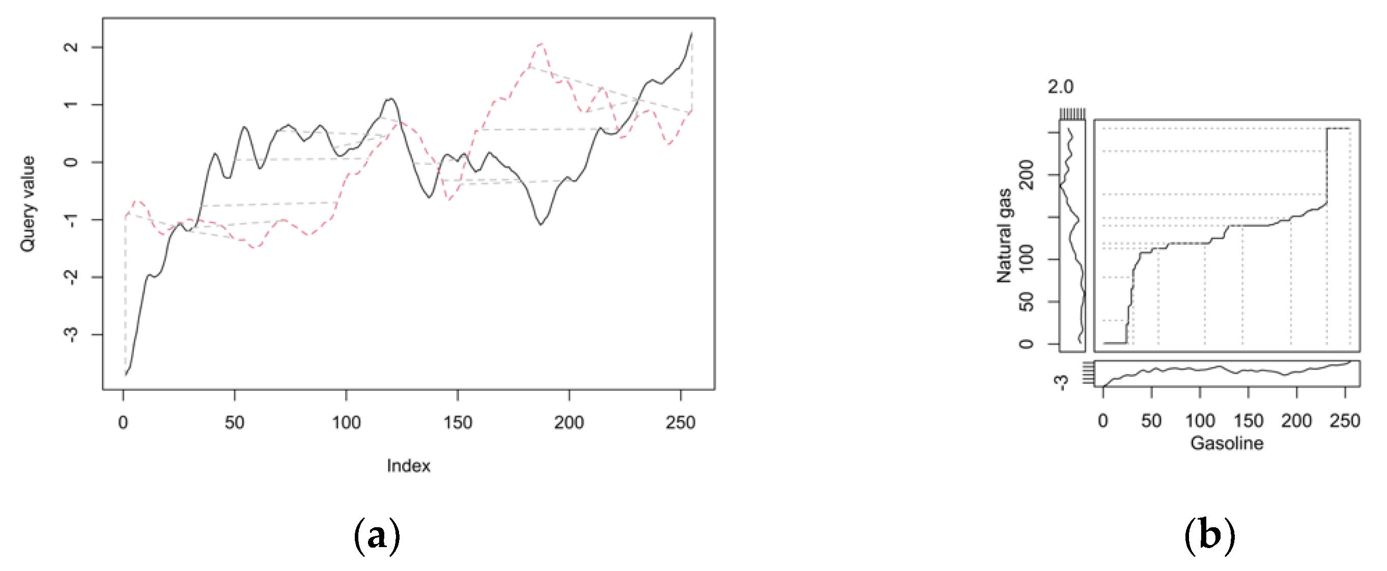
The pair of most different commodities with respect to time-series course in the whole period is gasoline and natural gas. This pair has the largest DTW distance, equal to 0.246. We present their two-way and three-way alignment plots in
Figure 6.
The courses of gasoline and natural gas prices are different to a large extent. Moreover, they have visible phase differences. In the first period, the price of natural gas is ahead of the price of gasoline. Next, at the time of declaration of the state of pandemic, there was a deep decline in the price of gasoline, which was followed about just above three months later by the price of natural gas. After less than three months, the price of natural gas noted a steep increase, which was followed by the price of gasoline after about two months. On the whole period, the median time difference between phases of both charts is equal to 5 days (phases of prices of the natural gas occur earlier).
4.2. First Subperiod (5 January 2020–27 April 2020)
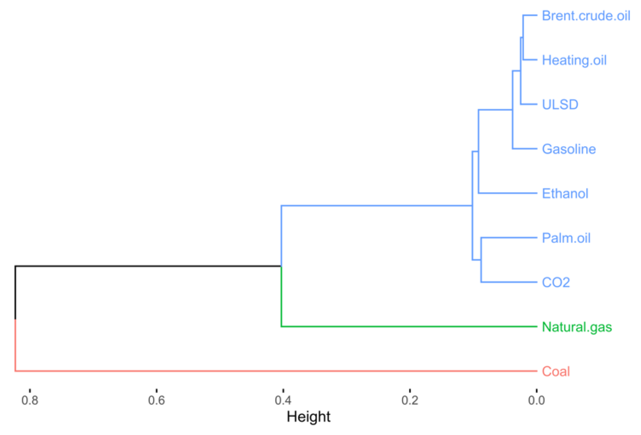
We present the dendrogram for the prices of analysed commodities in the first subperiod in
Figure 7.
In the first subperiod, we distinguish four clusters of commodities. However, three clusters are the ones with only one member—natural gas, CO2 allowances, and coal. All the remaining commodities create the fourth, large cluster. We obtain the same results for the k-medoids and divisive hierarchical clustering methods.
As in the case of the full period, ULSD and heating oil are the two most similar commodities in terms of their price developments in the first subperiod. The DTW distance between them is 0.017. We present their two-way and three-way alignment plots in
Figure 8.
The prices of both commodities have practically the same course. They are declining in the whole analysed subperiod. Only a very small discrepancy in their courses is visible after 90 days. The median phase difference is 0 days.
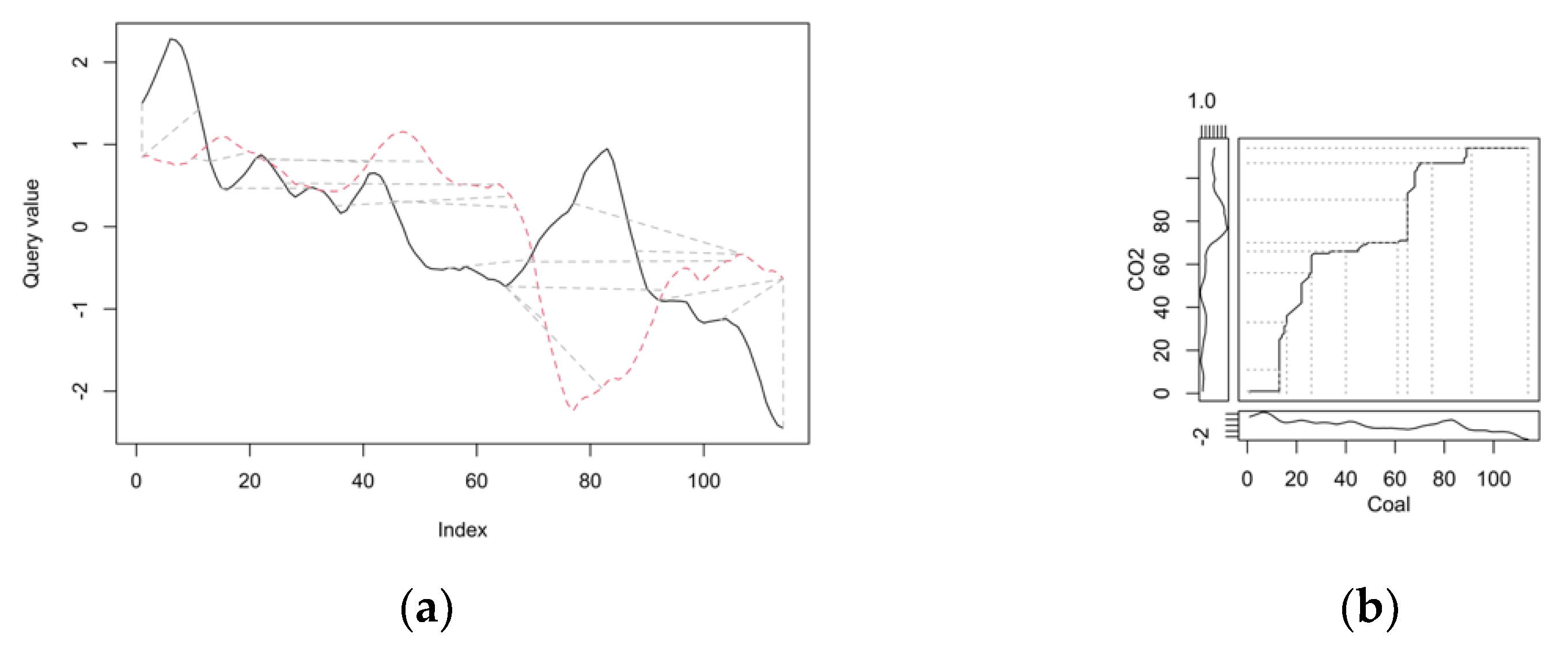
The most different pair of commodities consist of coal and CO
2 allowances prices. The DTW distance between them in the first subperiod is equal to 0.324. We present their two-way and three-way alignment plots in
Figure 9.
We can hardly see any similarities in courses of prices of coal and CO2 allowances. What is quite interesting is that the most visible fluctuations of prices of both commodities occurred in two directions. The biggest fluctuation for both of them takes place at more or less the same time, i.e., on the 80th day. The price of CO2 allowances decreases, while the price of coal at the same time increases. A similar (but to a much smaller degree) relation could be observed at the very beginning of the subperiod. The median phase difference between prices of coal and CO2 allowances is 20 days (phases of the prices of coal occur earlier). If we consider this shift, then the direction would be similar.
4.3. Second Subperiod (from 28 April 2020 to 7 January 2021)
In the period between the peaks of the first and second waves of the pandemic, a dendrogram for the prices of analysed commodities is presented in
Figure 10.
For the second subperiod, we distinguish the two clusters of commodities with respect to similarity of the courses of their prices. One cluster consists of only two commodities—ethanol and natural gas. All remaining commodities create the second cluster. We obtain the same results for the k-medoids and divisive hierarchical clustering methods.
The same, as in the full period and the first subperiod, commodities have the most similar courses of their prices in the second subperiod—ULSD and heating oil. The DTW distance between them was 0.018. We present their two-way and three-way alignment plots in
Figure 11.
As in the previous subperiod and the whole period, the dynamics of prices of ULSD and heating oil are virtually the same. In addition, there is no phase difference between them (median phase difference is equal to 0).
The two most different commodities in the second subperiod with respect to changes of their prices are gasoline and natural gas. The DTW distance between the time series of their prices is equal to 0.229. We present their two-way and three-way alignment plots in
Figure 12.
In the same periods, the directions of gasoline and natural gas prices are generally reversed (the period from the 30th to the 100th day and from the 150th day onwards). When we consider the median difference between the indices of both series (the gasoline indices are 3.5 days ahead), the picture does not change much. Between days 30 and 100, changes of the gasoline prices are ahead of changes of the natural gas prices, while between days 150 and 200, the opposite is true.
4.4. Third Subperiod (8 January 2021, Onwards)
The third subperiod covers the data from the peak of the second wave of the pandemic, until the end of the observation period. We present the dendrogram for the prices of analysed commodities in this subperiod in
Figure 13.
There are three visible clusters for the third subperiod. Two of them have just one member—coal and natural gas. All remaining commodities form the third, rather homogeneous cluster. The reason for this is that while the coal price is in this subperiod decreasing with high fluctuations, the natural gas price increases and then decreases, and the prices of all other commodities are generally increasing throughout the whole subperiod. We obtain the same results for the k-medoids and divisive hierarchical clustering methods.
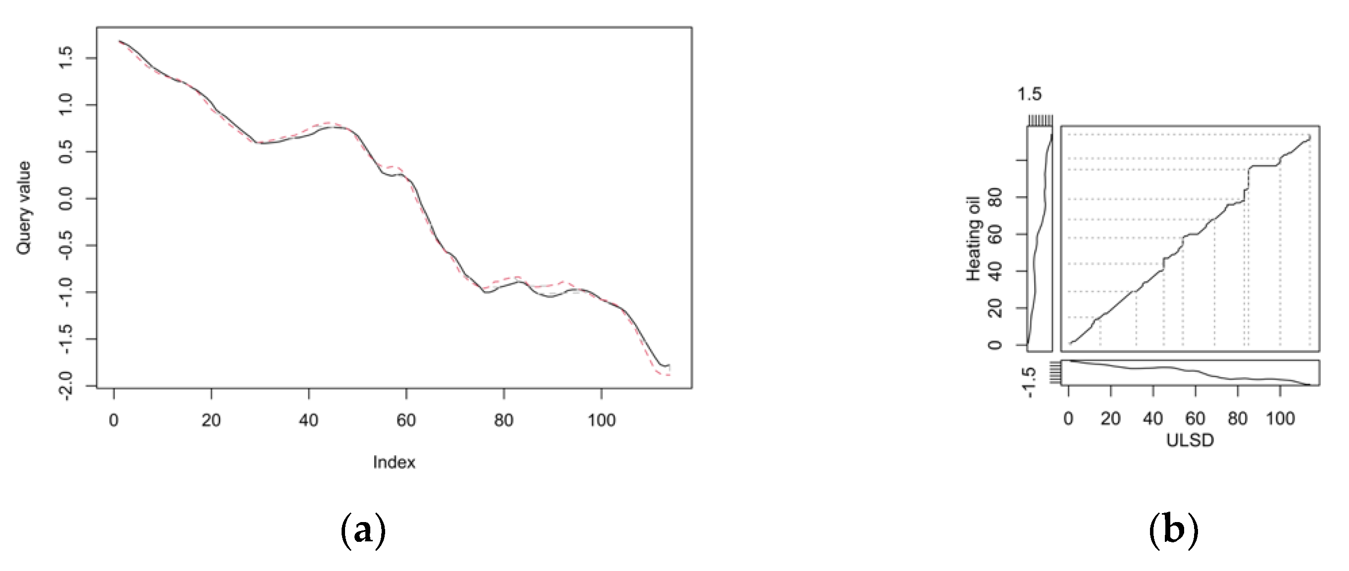
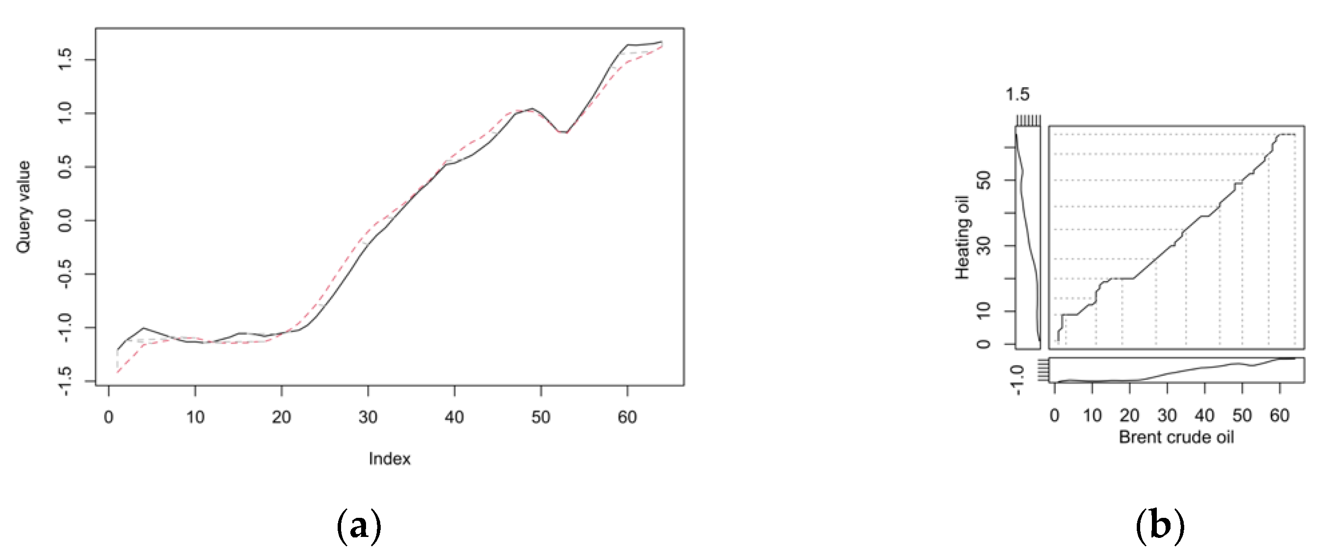
It is quite surprising that in the third subperiod, the two most similar commodities with respect to time series of their prices are not ULSD and heating oil (as in all previous situations) but crude oil and heating oil. The DTW distance between them is 0.021. We present their two-way and three-way alignment plots in
Figure 14.
The time series for Brent crude oil and heating oil in the third subperiod are very similar. However, their similarity is not as great as in the cases of previous subperiods and the whole period for the pair ULSD—heating oil. The higher DTW distance confirms this finding. The median phase difference for Brent crude oil and heating oil in the third subperiod is 0.
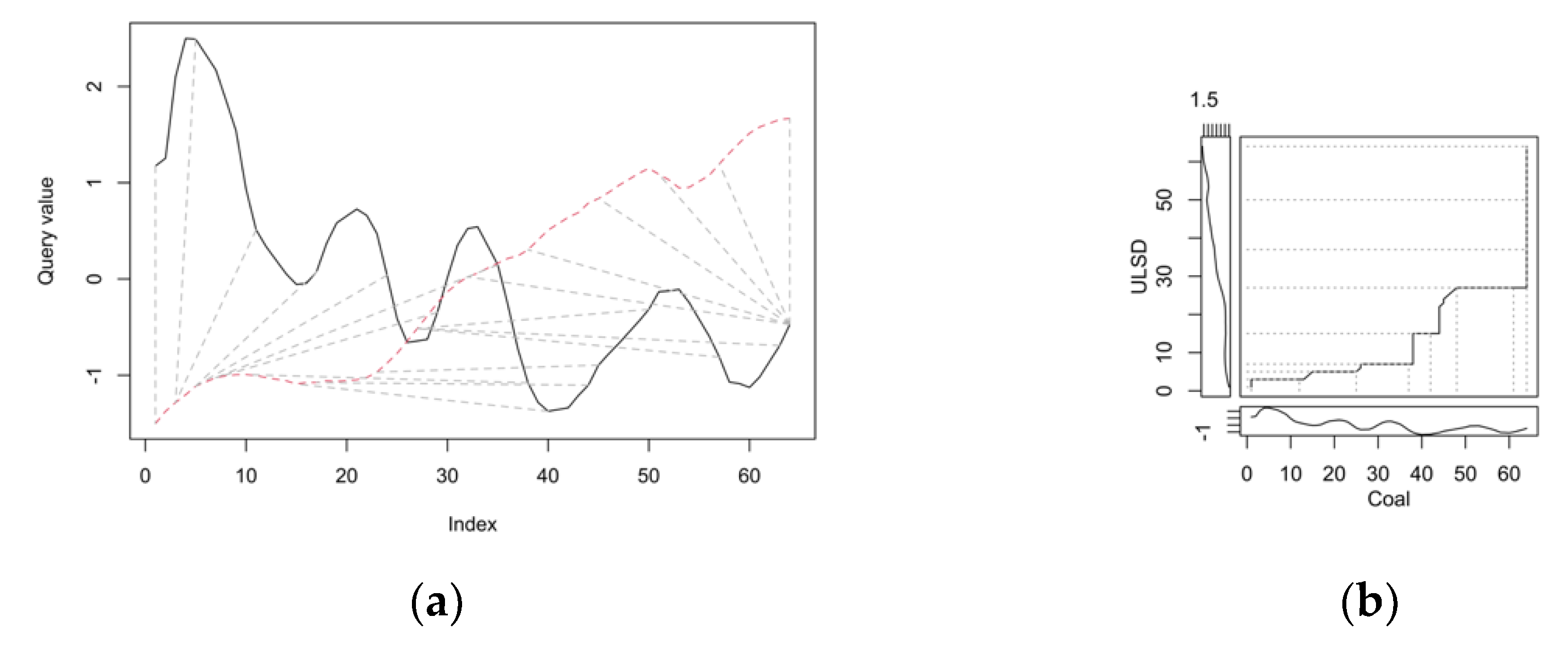
The two most different time series in the third subperiod are for the pair coal–ULSD. The DTW distance between them is 0.974. We present their two-way and three-way alignment plots in
Figure 15.
The time series of coal prices and ULSD for the third subperiod are almost completely different. Prices of ULSD increase throughout the analysed subperiod (with two small declines). On the other hand, the coal prices are decreasing with very strong fluctuations. The indices of coal prices are ahead of indices of the ULSD prices, which means that the time series for ULSD lead the time series for coal (with a median time of 22 days). However, it is impossible to talk about any shift between these two series—they are completely uncorrelated.
In the next step of the research, we analyse the similarities of time series for commodities prices to the time series of daily COVID-19 cases in the full period and three subperiods. The group with a distance smaller than the median is denoted by “A” and not smaller than median by “B”. We present the results in
Table 1.
The most similar time series of commodity prices to the time series of COVID-19 daily cases are the time series for palm oil and coal. The most dissimilar ones were gasoline, ethanol, and ULSD. Quite surprisingly, the heating oil prices for the second subperiod are in the group of more similar ones. It is worth noting that crude oil, heating oil, gasoline, ethanol, and ULSD prices are dissimilar to the COVID-19 daily cases for the whole period. They are also dissimilar for the first subperiod (the pandemic outbreak) and in the third subperiod. Some of them (heating oil and Brent crude oil) are amongst the more similar ones in the second subperiod. We might explain it by the fact that the prices of these commodities react strongly to the declaration of the pandemic state—as the number of COVID-19 cases is increasing, the prices of these commodities fall sharply. In the second subperiod, when the global markets have somehow become accustomed to the situation, in some cases, these differences are not so visible. The situation in the third subperiod is similar to the first one—the changes in the prices of these commodities have different directions than the changes of the daily COVID-19 cases.
The remaining commodities—CO2 allowances, natural gas, palm oil, and coal—have prices that react much weaker to the pandemic. Therefore, their time series are more similar to the daily COVID-19 series than the series that react to them in the opposite directions.
Eventually, we analysed the time shifts between the daily COVID-19 cases and commodities prices. We present the median differences between the indices of the compared time series in
Table 2. Negative values mean that the COVID-19 time series is ahead of the commodities series (the COVID-19 time series leads the commodity series), and positive values mean the opposite.
For the whole period, the median differences between indices of the COVID-19 daily cases and the commodities indices are negative. The biggest difference (the largest time shift) concerns the prices of ULSD and heating oil—over two months. This means that the time series of the COVID-19 cases leads the prices of these two analysed commodities, and the prices of these commodities follow the similar direction as the COVID-19 daily cases after more than two months. The smallest difference (11.5 days) occurs in the case of natural gas.
In the first subperiod, the situation is similar as in the whole period—the COVID-19 time series is ahead of the time series for prices of all commodities. These differences are generally smaller than for the whole period, with three exceptions: natural gas (for which it is the biggest—1.5 months), ethanol, and palm oil. It is caused by the reaction of commodity prices (first falling, then rising) to the increase in daily COVID-19 daily cases.
The second subperiod is characterised by much smaller values of the time shift between the time series of the COVID-19 daily cases and prices of commodities. However, the biggest difference between this and the first subperiod is the opposite sign of this shift. When we combine this with the fact that the DTW distances between the time series of commodities prices and the COVID-19 daily cases are the smallest, it turns out that in this subperiod, the time series for commodities are much more similar to the COVID-19 time series than in the first subperiod. A smaller time shift also means that the directions of compared series are largely the same. We can also interpret it as the markets becoming accustomed with the pandemic situation.
The third subperiod is characterised by higher values of time shift between the prices of commodities and the COVID-19 daily cases (with the exception of coal). However, all median values are positive for this period, which means that the time series for commodities overtook the time series of daily Covid-19 cases. This can be the manifestation of the situation that the markets anticipate the pandemic evolution. Epidemiologists, doctors of infectious diseases, predict courses of the pandemic; therefore, the changes on the markets could happen earlier than changes of Covid-19 cases.
In the case of the energy commodity market, the analysis of oil and gas prices in particular has received considerable attention. Our research results show that gas and oil prices differ from COVID-19. Similar results have been obtained by other researchers. Nyga-Łukaszewska and Aruga [
40] show that in the USA, the cumulative number of COVID-19 cases has a statistically negative effect on the oil price, while it has a positive effect on the gas price. In Japan, this negative impact is only seen in the oil market with a two-day lag. The number of cases has no effect on the Japanese oil and gas markets. The authors explain their findings by the fact that the spread of the virus is different in the two compared countries and the measures taken by the governments to prevent the epidemic are different.
When examining the similarities in the evolution of energy commodity prices, we can see that in each subperiod natural gas differs from the other commodities (generally, it forms a distinct cluster). This is confirmed by Lin and Su [
14], who show that natural gas prices are the least correlated with the prices of other commodities. This is the case both before and during the pandemic. The study also confirms the very strong correlation between heating oil and diesel price.
Analysing the time series of selected energy commodities, an initial decline in prices is evident, followed by an increase. This is consistent with the predictions of Liu, Wang, and Lee [
77], who indicate the existence of a negative relationship between oil and stock returns. However, they find that the COVID-19 pandemic outbreak can have a significantly positive impact on oil and stock market returns. They even suggest that there is no need for governments to take actions to avoid the possible negative impact of the pandemic on the oil and stock market in the short term.
The DTW method we use is widely applicable for determining the distance (similarity) matrix between time series. Classification or clustering based on the distance matrix between time series belongs to distance-based methods [
78]. There are many possible distance measures and methods for clustering or classification. Bagnal et al. [
79] compare 18 different time-series classification techniques. Classifications based on the DTW method are always among the best.
5. Conclusions
After falling in early 2020, energy prices rebounded. Later, the combination of production cuts and a pickup in consumption helped prices to recover. To this day, the energy commodities have recouped their losses from the COVID-19 pandemic. Almost all analysed commodity prices are now above prepandemic levels.
In our research, we examine the similarity between the time series of energy commodity prices and the time series of daily COVID-19 cases. The most similar to the COVID-19 are the time series for coal and palm oil, and the most dissimilar for gasoline, ethanol, and ULSD. The analysis carried out over three subperiods shows that the Brent crude oil and heating oil prices react strongly to the outbreak of the pandemic. This confirms hypothesis H2. As the global markets adjust to the situation, the changes in the prices of these commodities are more similar to the changes in the daily COVID-19 cases. However, the price evolution in the third analysed subperiod is in the opposite direction to the changes in the number of infected individuals.
In addition, the time shifts between the daily COVID-19 cases and commodities prices are analysed using the dynamic time warping method. In the first subperiod, the time series of the COVID-19 cases lead the prices of all energy commodities. The smallest time shift concerns the prices of coal; the largest is noted for natural gas. In the second and third subperiod, the markets become accustomed to the pandemic situation, and the shifts have the opposite sign, which means that the time series for energy commodities precede the time series of COVID-19 cases. It seems that at this stage of the pandemic, the markets anticipate its evolution. Thus, the hypothesis H1 is confirmed partially, only for the first subperiod of the analysis.
Our analysis also allows the grouping of energy commodities using a hierarchical clustering algorithm. We distinguish commodity clusters with respect to the three analysed subperiods. In general, it can be stated that commodities such as ULSD, heating oil, crude oil, and gasoline form a group weakly related to COVID-19, while coal, natural gas, palm oil, CO2 allowances, and ethanol are strongly connected.
We are aware of the limitations of the research methodology we have adopted. Its biggest limitation is that, based on it, we are not able to investigate what variables/phenomena directly affect the prices of energy commodities we analyse. The increase in COVID-19 cases resulted in the introduction of restrictions by country authorities, which disrupted the movement of goods and people, resulting in reduced mobility. During the first wave of the pandemic, production in some industries was also suspended, resulting in a drop in demand for energy and fuel. Investor sentiment in capital markets also deteriorated. All these phenomena directly affected the prices of energy raw materials. In order to study this impact in detail and assess its significance, econometric models with control variables would need to be built, and causality can be inferred from them. The fact that the issue of the impact of pandemics on various socioeconomic phenomena is very important is demonstrated by the number of scientific publications appearing on the subject. The link between the development of the pandemic and these phenomena can be investigated using a number of methods. Many of these studies are presented in the literature review.
Our research does not aim to find the exact relationships between the prices of the energy commodities and COVID-19-related phenomena (we can find many such analyses in the literature). We aim to find connections and similarities between the development of the pandemic (measured by the number of new COVID-19 cases) and the prices of the energy commodities. By these means, we can find the commodities for which the dynamics of their prices is the most similar to the course of the pandemic. In our case, there are the prices of coal, palm oil, and, to a lesser degree, the prices of CO2 allowances and natural gas. Knowing this, we may expect that the prices of these commodities would be affected by similar occurrence in the future. In addition, our framework can be used for other types of commodities (e.g., metals, agricultural products, or prices on real estate markets). This is a future direction of our research. Our further research plans also include building econometric models for energy commodity prices with control variables.


