Article

Heat Transfer Efficiency Prediction of Coal-Fired Power Plant Boiler Based on CEEMDAN-NAR Considering Ash Fouling

1
School of Electrical and Control Engineering, North University of China, Taiyuan 030051, China
2
School of Data Science and Technology, North University of China, Taiyuan 030051, China
*
Authors to whom correspondence should be addressed.
Energies 2021, 14(13), 4000; https://doi.org/10.3390/en14134000
Submission received: 1 June 2021 / Revised: 24 June 2021 / Accepted: 25 June 2021 / Published: 2 July 2021

Abstract

:
Ash fouling has been an important factor in reducing the heat transfer efficiency and safety of the coal-fired power plant boilers. Scientific and accurate prediction of ash fouling of heat transfer surfaces is the basis of formulating a reasonable soot blowing strategy to improve energy efficiency. This study presented a comprehensive approach of dynamic prediction of the ash fouling of heat transfer surfaces in coal-fired power plant boilers. At first, the cleanliness factor is used to reflect the fouling level of the heat transfer surfaces. Then, a dynamic model is proposed to predict ash deposits in the coal-fired boilers by combining complete ensemble empirical mode decomposition with adaptive noise (CEEMDAN) and nonlinear autoregressive neural networks (NARNN). To construct a reasonable network model, the minimum information criterion and trial-and-error method are used to determine the delay orders and hidden layers. Finally, the experimental object is established on the 300 MV economizer clearness factor dataset of the power station, and the root mean square error and mean absolute percentage error of the proposed method are the smallest. In addition, the experimental results show that this multiscale prediction model is more competitive than the Elman model.

Graphical Abstract

1. Introduction

Fossil fuel power plants play an important role in providing energy all over the world, even though renewable power has been greatly developed in recent decades. Coal is one of the major fossil fuels. Coal-fired power generation capacity still accounts for 51.2 percent of total installed capacity in China by the end of June 2020, and the coal-fired generation accounts for 72.3 percent of the total power generation in China in the first half of 2020 [1]. Energy conservation and emission reduction is an important practical problem in the sustainable development of economic society in the world. Therefore, energy conservation and emission reduction of coal-fired power plants are particularly critical.
Coal is the energy source of coal-fired power plants, but the following problems still exist: When the pulverized coal obtained by the coal mill is burned in a furnace, the high-temperature flue gas produced will act on the working medium side of the heating surface in the way of heat transfer, and the ash in the high-temperature flue gas will be carried in the melting state after exceeding the melting point, leading to ash accumulation on the heating surface with the flow of high-temperature flue gas. Large boilers generally have the characteristics of large parameters and power, and this kind of ash accumulation will be more obvious and become an urgent problem to be solved. Because the thermal resistance of the ash is much greater than that of the metal heating surface, to heat the working fluid will inevitably cause more raw coal consumption, which may further cause the corrosion of the heating surface and the metal pipeline and significantly reduce the service life of the equipment. In addition, due to the poor heat absorption capacity of the heating surface, the boiler tail outlet smoke temperature is high, so the flue gas desulfurization rate is reduced [2,3]. It has been estimated that ash deposition can reduce the amount to 1 percent of boiler efficiency under the normal operating conditions in coal-fired power plant boilers [4]. Therefore, how to realize the ash monitoring and soot blowing optimization of the coal-fired power plant has become a hot topic and has become more relevant [5,6,7,8]. It is still a challenge because there are a lot of factors that affect the deposition of ash. Even ash fouling in the same heat transfer surface will have a different trend in the actual production process. Therefore, it is necessary to monitor the ash fouling of heat transfer surfaces and formulate corresponding soot blowing strategies to ensure the safety, reliability, and economy of coal-fired power plant boilers.
Soot blowing is a common method used to clean the ash fouling on the heat transfer surfaces to ensure the heat transfer efficiency at a high level. The commonly used medium for soot blowing mainly includes steam [9], acoustic waves [10,11], etc. At present, many coal-fired power plants still adopt the unscientific soot blowing strategy with fixed duration or fixed threshold as reference. It is necessary to optimize the soot blowing duration and threshold. Wen et al. [3] used the Hamilton–Jacobi–Bellman Equation (HJB) to study the optimal soot blowing strategy for a boiler system with the variable steam flow. The continuous-time Markov process with flue gas deposition mode and the soot blowing model is used as the mathematical model of the system, the dissipation function is designed for the established boiler model, and the HJB Equation is solved accordingly to obtain the corresponding value function as the optimal ash blowing strategy. Based on the optimization of the optimal soot blowing cycle and the ash pollution monitoring, Shi et al. [12] proposed real-time soot blowing time optimization method, which can be used to optimize the termination time of the soot blowing operation. In order to make the coal power plant have a better economic benefit, prepare for soot blowing operation and avoid the occurrence of safety accidents, it is crucial to determine the degree of fouling of heated surfaces.
Prognostics and Health Management (PHM) is used to predict the degradation in industrial devices and then give the optimal maintenance plan [13,14]. PHM of ash fouling of heating surfaces in coal-fired power plant boilers is mainly divided into three processes, i.e., ash fouling monitoring, ash fouling prediction, and soot blowing optimization. Ash fouling monitoring is the basis of the prediction and soot blowing optimization. Ash fouling not only depends on the ash content of coal but also depends on the distribution of heat transfer surfaces, combustion status, flue gas velocity, and many other factors. Due to the complex structure of the heat transfer surfaces, it is difficult to measure the condition of the ash fouling directly. It is usually expressed indirectly by the heat flux or the heat transfer efficiency of the heating surfaces, e.g., heat flux meter [15] and acoustic pyrometry [16]. However, due to the high price and the need for pre-installation, some power plants without conditional installation cannot be used. In this study, an indirect representation called the cleanliness factor (CF) was used to monitor the ash fouling status of the heating surfaces of the coal-fired power plant boilers [12].
There are many studies on ash fouling monitoring and prediction. These methods can be divided into three categories including model-based, data-driven, and hybrid methods [17,18,19]. The model-based method is widely studied, which is mainly to analyze the mechanism of ash fouling and establish a mathematical model to characterize the increase in the thickness of the ash [20]. However, due to the complexity of the change of ash fouling of heating surfaces being affected by many factors, it is difficult to establish an accurate mechanism model. Data-driven approaches have received more attention recently. By using the historical data of ash fouling in the superheaters [21], reheaters [22], and air preheaters [23], the exponential curves of ash accumulation and soot blowing stage were fitted to predict the future trend of ash accumulation and degradation. However, these models are difficult to extend to other heating surfaces or even to the different stages of the same heating surface. Ma et al. [24] used CFD to simulate the location of the ash fouling on the heating surface and compared it with the measured results to verify the model in order to predict the ash fouling on the heating surfaces. However, the time of CFD simulation calculation is too long to achieve real-time prediction, which is not suitable for real-time monitoring of the ash fouling on the heating surfaces of coal-fired power plant boilers. Perez et al. [10] considering the global response time of the system in the polluted state and, comparing it with the clean state, designed a new transient thermal fouling probe for cross flow tubular heat exchangers, which accurately estimated the convection exchange coefficient and the degree of fouling of the heat exchanger. At present, many methods are based on artificial neural network technology [25], regarding the ash deposition system as a ‘black box model’, and complete the prediction of ash accumulation and integrated optimized automatic smoke blowing control. Li et al. [26] decomposed the historical pollution rate data into two parts, the fitted curve data and the difference between the original data and the fitted curve. Combining real-time pollution rate data, a prediction model is established. Compared with the traditional Elman neural network, the prediction accuracy is significantly improved. Tong et al. [8] found 20 fouling-related variables and used SVR to complete the nonlinear mapping relationship between fouling factor variables and actual fouling conditions (characterized by the thermal resistance of the ash layer calculated by the thermal balance mechanism model). On the test set, an accuracy rate of 98.5 was achieved. Li et al. [27] used a deep learning model to predict ash accumulation. Compared with the shallow model, it highlights its advantage of mining the long-term dependence of time series and obtains higher prediction accuracy.
The neural network (NN) can approach the complex nonlinear model and achieve better accuracy for prediction. NN not only simulates the human brain but also knowledge accumulation in the process of learning [28,29,30]. The proposed methods use a neural network to predict the ash fouling on the heating surface, mainly through the establishment of an artificial neural network prediction model. These neural network models are usually trained with historical data and then used to monitor or predict the trend of ash fouling. The static model is difficult to describe the dynamic characteristics because the actual ash fouling and soot blowing processes are dynamic.
This paper presents a dynamic NN method, which uses Elman neural network (Elman) with neural feedback characteristics and nonlinear autoregressive neural network (NARNN) to build the model to predict the ash fouling of heating surfaces in coal-fired power plant boilers. At first, the cleanliness factor was used to characterize the ash fouling status. Furthermore, a dynamic neural network based on combined complete ensemble empirical mode decomposition with adaptive noise (CEEMDAN) and dynamic model (NARNN and Elman) is proposed to predict ash fouling. The minimum information criterion and trial-and-error method are used to determine the delay orders and hidden layers, which can reduce the training time and improve the prediction accuracy. Though the actual data of 300 MW economizer in a thermal power plant are experimentally studied, the reliability and superiority of the proposed method are verified by setting a variety of rolling prediction steps and different starting point predictions, results show that the method has sufficient accuracy and high practical value.
The outline of our paper is as follows. The problem statement is presented in Section 2. The methodology of decomposition algorithm and dynamic network is introduced in Section 3 and Section 4. The results are analyzed and discussed in Section 5. Finally, conclusions are drawn in Section 6.

2. Problem Statement

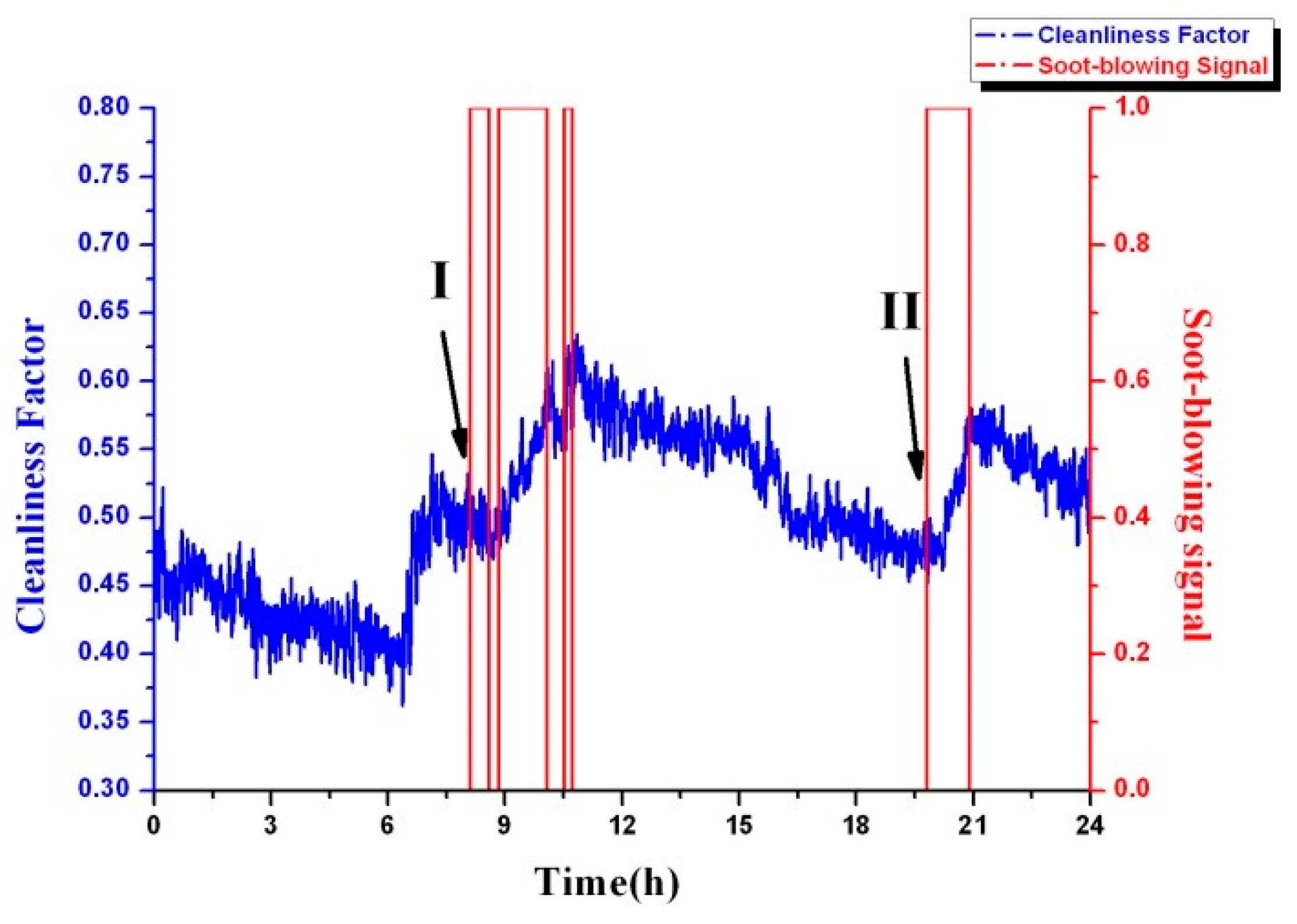
2.1. Cleanliness Factor

In this paper, the cleanliness factor (CF) is used as a health factor to characterize the ash deposition state of the conventional heating surfaces in the coal-fired power plant boiler, which is a sign of the cleanliness of the heating surface. The ratio of the actual heat transfer coefficient to the ideal heat transfer coefficient is defined, as shown in Equation (1) below [16].
C F = h r h o
where h r and h o are the actual and theoretical heat transfer coefficients of the heating surface respectively. CF is the fouling rate and is dimensionless. Obviously, the value of CF lies in the interval [0, 1], with one representing the most primitive ideal cleaning condition of the heating surfaces.
CF is obtained from the online monitoring model of the heating surface. First, the composition of the flowing gas is calculated by using the coal composition, primary airflow, secondary airflow, fuel flow, and combustion model. Available temperature, pressure, and mass flow in the steam and gas sides allow the heat transferred in the boiler to be calculated by means of mass and energy balance in each heat transfer surface. In addition, the heat transfer efficiency of the heating surface is also related to the change of load, so the dynamic mass and energy balance method are adopted to avoid the impact of unexpected circumstances. Then, h r is obtained, and the h o is obtained through the theoretical thermal calculation method.
The theoretical heat transfer coefficient is the original state without ash deposits on the heated surface. Under the premise of ignoring the thermal resistance of the working fluid and the tube wall and the internal resistance of the metal, it is usually the sum of the theoretical radiation heat transfer coefficient and the theoretical convective heat transfer coefficient.
h o = a f + a d .
In the equation, a f represents the theoretical radiation heat transfer coefficient, and a d is the theoretical convective heat transfer coefficient. The following equation is the specific mechanism equation of the two heat transfer coefficients [23]:
a f = 5.7 × 10 8   a g b + 1 2   a h T 3 K
a d = 0.65   C s C z λ d ( w d v ) 0.64 P r 0.33
K = { ( 1 ( T g b T ) 4 ) / ( 1 T g b T ) } .
In the equation, a g b and a h are the emission coefficients; T , T g b are the temperature of the flue gas and the pipe wall respectively, C s , C z are the transverse and longitudinal directions of the heating surface, λ is the thermal conductivity of the flue gas, and d is pipe diameter, w is the flue gas flow rate, v is the dynamic viscosity of the flue gas, and P r is the Reynolds number.
The flue gas flow rate w is the ratio of the flue gas flow rate to the area of the tube section of the heating surface.
w = V b A
where V b is the standard flue gas volume passing through the heating surface, A is the official cross-sectional area of the heating surface, and the standard flue gas flow rate is obtained by Avogadro’s law.
V b = ρ r V r ρ b / ( 1 + t r 273.15 )   .
In the equation, V r is the measured flue gas flow through the heating surface, t r is the flue gas temperature through the heating surface, ρ r is the actual pressure of the flue gas, and ρ b is the standard atmospheric pressure.
The actual heat transfer coefficient is obtained by dynamic energy balance and iterative method.
h r = Q y F Δ t m
Δ t m = ( Δ t m a x Δ t m i n ) / l n Δ t m a x Δ t m i n
where Q y is the energy released on the flue gas side, F is the heat transfer area of the heating surface, Δ t m is the average heat exchange temperature difference between the flue gas side and the working fluid side, and Δ t m a x and Δ t m i n are the maximum and minimum temperature differences of heat exchange on both sides.
Considering that during the operation of the boiler, as the load changes, the boiler’s coal feed, air supply and other variables are dynamically changing, and the corresponding temperature of each heating surface is also changing, and the specific heat capacity of the working fluid will also change with the change of temperature. Therefore, the energy released by the flue gas side in the dynamic process is not completely equal to the heat absorbed by the working fluid. At this time, the change in the heat storage of the working fluid needs to be considered. Therefore, the energy conservation on the flue gas side and the working fluid side in this dynamic process can be expressed as
Q y = Q q ± Δ Q j ± Δ Q q
where Q q is the heat absorption of the working fluid on the working fluid side, Δ Q j is the change in the heat storage of steam, and Δ Q q is the heat absorption change on the steam side.
Heat release on the flue gas side:
Q y = φ B j ( h i n h o u t + β h l f )  
B j = B ( 1 q 4 100 )  
φ is the heat retention coefficient, h i n and h o u t are the flue gas enthalpy values at the inlet and outlet of the economizer, β is the air leakage coefficient of the flue section, and h l f is the cold air enthalpy of the air leakage, B j is the calculated fuel quantity, B is the actual measured fuel quantity entering the furnace, and q 4 is the heat loss of the mechanical incomplete combustion of the boiler.
The metal heat storage change of the pipe wall, the steam heat storage change, and the heat absorption of the steam side are as shown in the equations.
Δ Q j = C j m j θ j τ
Δ Q q = C q m q θ q τ
Q q = D ( H o u t H i n ) .
In the equation, C j and C q are the average specific heat capacity of metal and working fluid respectively. m j and m q are the metal quality of the tube wall on the heated surface and the quality of the working fluid inside. θ q and θ j are the metal pipe wall temperature and steam temperature, D is the mass flow of the working fluid of the economizer, H o u t and H i n are the side enthalpy values of the working fluid in and out of the economizer. The enthalpy value of the working fluid can be obtained by the international general industrial water and water vapor property calculation formula.
The CF monitoring results of an economizer in a 300 MW coal-fired power plant are shown in Figure 1 as an example. The two points I and II with obvious increase correspond to the real soot blowing signals. There is a slow and obvious decreasing process of CF between the point I and point II, which represents the decrease of heat absorption capacity of heating surfaces caused by ash deposition. Therefore, the cleanliness factor can be used to describe the degree of fouling of boiler heating surfaces. The change rule of the cleaning factor obtained by the model is consistent with the actual theoretical analysis, which is sufficient to prove the accuracy of the model.

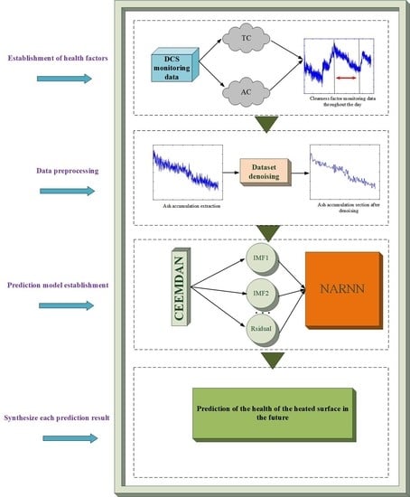
2.2. Data Preprocessing

The design of intelligent soot blowing needs to be based on the prediction of heating surfaces of the boiler. At present, the data indicating the degree of ash deposition cannot be obtained directly on the heating surfaces, but can only be calculated by various indirect data to represent the state of ash deposition. However, before characterizing the ash level of the heating area, the original data is collected through the DCS of the coal-fired power plant. There will be some numerical errors in the cleaning factors obtained according to the calculation formula, which need to be processed on the data. Figure 2 shows the raw data displayed in the DCS database and the results of the data processing. The final data collection period is the 50 s, but the trend of ash deposition cycle data is not affected. Due to the objective of the study in this article, only the fouling section of the cleaning factor is intercepted. It can be seen from Figure 2 that when the economizer is working normally, the cleanliness of its heating surfaces continues to deteriorate over time, and the value of the cleaning factor is also continuously decreasing.

3. CEEMDAN

Empirical Mode Decomposition (EMD) is proposed by the National Aeronautics and Space Administration (NASA), N.E. Huang, and others, which decompose nonlinear and nonstationary signals into different eigenmode functions [31]. As a signal adaptive analysis method, the EMD algorithm completely relies on the signal itself to adaptively determine the number of modal components obtained by decomposition, which overcomes the problem of selecting wavelet basis functions and decomposition scales for wavelet decomposition. However, it also has many problems, among which the aliasing mode is one of them. The flow of the EMD algorithm is as follows:
Step 1:
Connect all local extreme points in x ( t ) with cubic spline interpolation curves to form an upper and lower envelope and m l o w .
Step 2:
Mean curve of the envelope m 1 ( t ) = [ m u p + m l o w ] / 2 .
Step 3:
Recalculate the difference h 1 ( t ) = x ( t ) m 1 ( t ) . If it does not meet the two sufficient conditions of the intrinsic mode function (IMF) component, replace h 1 ( t ) with x ( t ) , and repeat steps 1 and 2 until h 1 k ( t ) meets the two conditions after k iterations.
Step 4:
The IMF1 component is c 1 ( t ) = h 1 k ( t ) , and the corresponding remaining component is r 1 ( t ) = x ( t ) c 1 ( t ) .
Step 5:
Repeat the above steps to decompose the residual component r 1 ( t ) as the original sequence, and finally obtain n IMF components and a residual component r n ( t ) , where the residual component is a monotonic sequence or a constant sequence.
Step 6:
The final EMD decomposition formula is shown in Equation (16)
x ( t ) = i = 1 n c i ( t ) + r n ( t ) .
The EEMD algorithm, as an improved method of the EMD algorithm, is a noise-assisted analysis method that solves the problem of modal aliasing by adding white noise to the original signal. The CEEMDAN method further reduces the modal effect by adding adaptive noise and has better convergence [32]. Compared to the commonly used EEMD method, it effectively reduces the number of iterations, increases the reconstruction accuracy, and is more suitable for the analysis of nonlinear signals. The CEEMDAN algorithm performs multiscale decomposition of the denoising cleaning factor degradation curve to achieve data stabilization and lay an important foundation for high-precision prediction.
In this paper, the economizer ash accumulation curve after filtering and smoothing still has the characteristics of strong nonstationarity and nonlinearity. This is because when the flue gas carrying ash flows through each heating surface, the faster flue gas flow rate will take away part of the soot on the heated surface, while the slower flue gas flow rate will deposit the soot in the flue gas on the heated surface, so that the heated surface pollution degree is aggravated. The flow rate of the flue gas causes the CF curve to have strong nonlinearity and nonstationarity (deposition and erosion of ash) even after the noise is removed, which is exactly the difficulty of prediction. If the neural network algorithm is used for direct prediction, it may not be able to adapt to multiple features at the same time.
On the basis of solving the modal mixing problem existing in EMD, CEEMDAN completed the multiscale analysis of the ash accumulation curve with multifeature fusion and obtained a global degradation component and several high-frequency components. The advantage of this is that the prediction model can better adapt to the input signals. Compared with wavelet decomposition algorithms, CEEMDAN has the advantages of self-adaptive determination of basis function and decomposition layer number. In addition, the time cost is an issue to be considered for multi-step-ahead predictions. Excluding the training time of the prediction model, the time occupied by CEEMDAN is less than 10 s, which is satisfactory.

4. Dynamic Neural Network

4.1. Elman Neural Network

Elman neural network is a classical dynamic network, which consists of the input layer, hidden layer, undertake layer, and output layer [33,34]. Compared with other feedforward neural networks, its main characteristic is that there is an additional connection layer in the structure, which constitutes the local feedback. This undertakes layer can be used as a delay operator, which enables the system to adapt to time-varying characteristics and dynamic memory, so it is very suitable for time series prediction. Its structure is shown in Figure 3a.
According to the neural network model, the mathematical model formula of Elman neural network is as follows
y ( t ) = g ( w 3 x ( t ) )
x ( t ) = f ( w 1 x c ( t ) + w 2 ( u ( t 1 ) ) )
x c ( t ) = x ( t 1 )
where y is the output node vector of dimension; x is the node element vector of n dimension intermediate layer; u is the input vector of r dimension; x c is n dimensional feedback state vector; w 3 is the connection weight from the hidden layer to the output layer; w 2 is the connection weight from the input layer to the hidden layer; w 1 is the connection weight from the undertake layer to the hidden layer; g ( ) is the linear combination of the transfer function of output neurons and the output of hidden layer. f ( ) is the transfer function of hidden layer neurons.

4.2. Nonlinear Autoregressive Neural Network

NAR (nonlinear autoregressive) neural network model is a nonlinear autoregressive model [35,36]. The autoregressive model is a nonlinear regression model using itself as a regression variable, i.e., using the linear combination of random variables at some early moments to describe random variables at some later moments. This is a common form of time series, which can be expressed as Equation (20)
y ( t ) = a 0 + a 1 y ( t 1 ) + + a n ( t ) y ( t n ) + e ( t )
where, e ( t ) is white noise. Based on this principle, the NAR neural network model adopted in this paper is a dynamic neural network based on time series, which can be defined as shown in Equation (21)
y ( t ) = f ( y ( t 1 ) , y ( t 2 ) , , y ( t d ) )
where, y ( t ) represents the output data at the current moment; y ( t 1 ) , y ( t 2 ) , , y ( t d ) represents the output data of historical moment; d represents the order of delay, and y ( t ) represents the network output. NAR neural network is composed of input layer, hidden layer, output layer and input delay order. As shown in Figure 3b.

4.3. Network Structure Design

The dynamic neural networks can be divided into two types according to different methods of realizing system dynamics. One is the regression network, which is composed of static neurons and output feedback of the network (such as NARNN). Another type is formed by neuronal feedback (e.g., Elman). In order to achieve the final long-term effective prediction results, it is no longer limited to the prediction with actual data. Therefore, this paper also designed Elman as output data feedback to the input layer, so as to form the network output feedback model. However, both neural networks need to design the number of input layers and hidden layers before they can be used.
Firstly, the number of neural network input can be divided into the following steps:
Step 1:
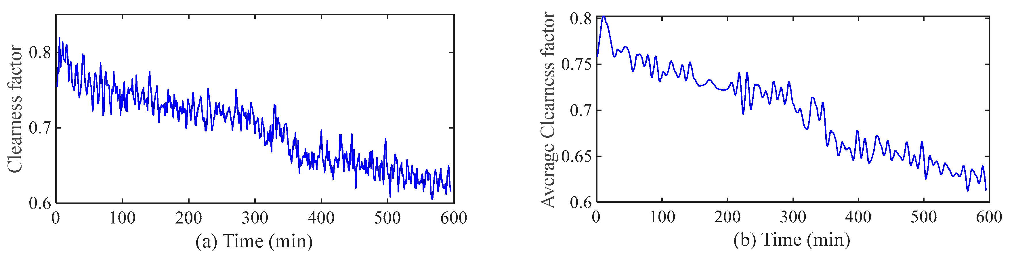
according to the ash accumulation data collected by DCS system under different working conditions, the average cleaning factor is obtained after processing the data, and the long sequence under different working conditions is tested to see whether it is a stationary sequence. ACF test or ADF test [37] unit root test is generally adopted.
Step 2:
after the stationary sequence is determined, all the sequences are detected by auto correlation, and partial correlation detection is carried out for all the sequences.
Step 3:
determine the input number or regression order according to Akaike information criterion.
Secondly, the best number of hidden layers is usually determined by empirical method. This paper uses trial and error method [38] to determine the optimal number of layers.
m = n + l + α m 4 n ( l + 3 ) + 1
where, m is the number of nodes of hidden layer; l is number of nodes in the input layer; α is number of nodes in the output layer;—integers between 1 and 10. According to Equation (22), the number of hidden layer nodes m is calculated to be between 4 and 13.
Finally, a complete neural network structure model is constructed. The optimal structure of Elman is n = 5 , m = 9 , the optimal structure of NARNN is d = 5 , m = 8 .

5. Results and Discussions

5.1. Dataset Description
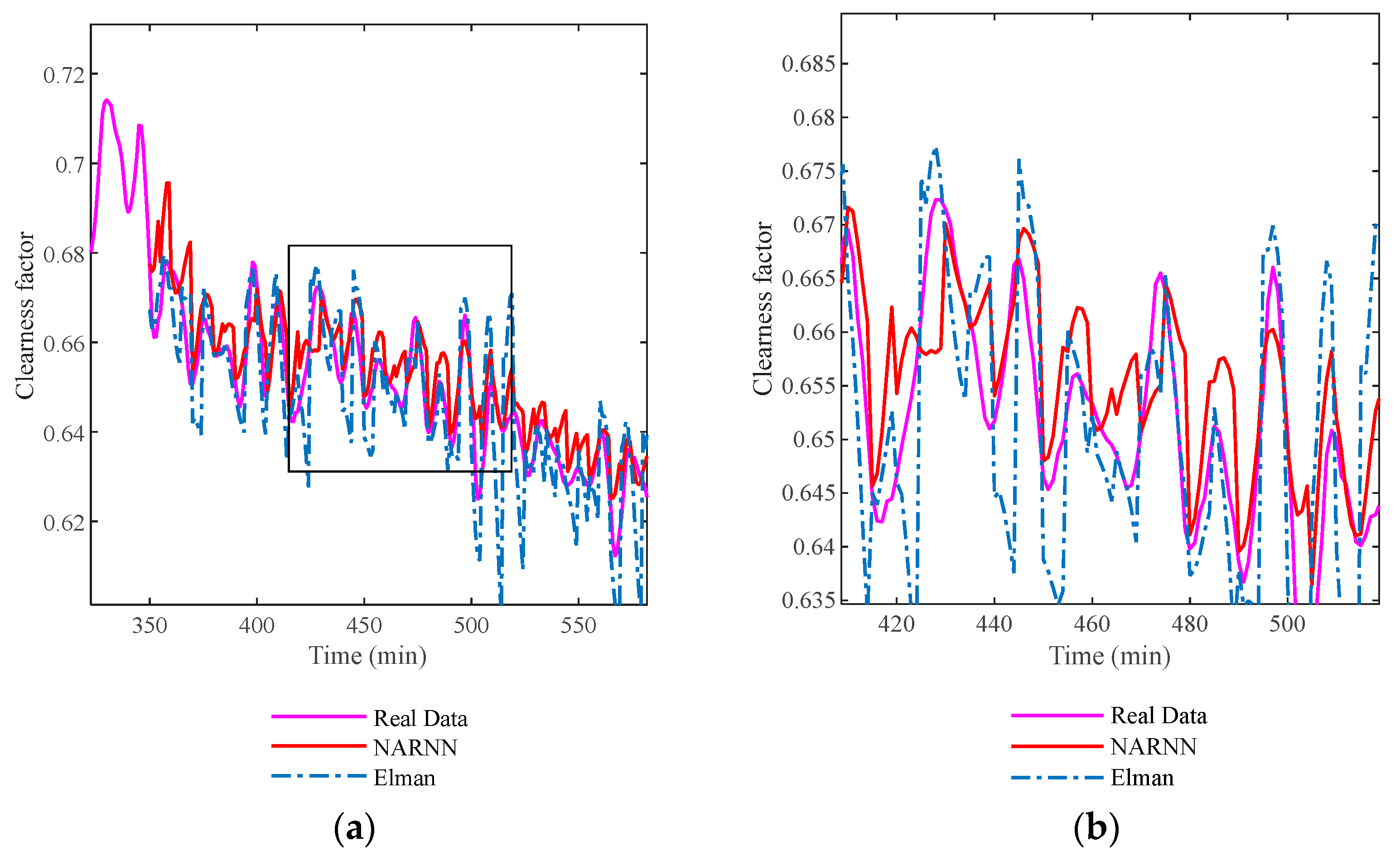
In order to verify the effectiveness of the proposed method, the CF data set of the 300 MW boiler economizer in the power plant described in Section 2 is used in this paper [23]. The coal is lignite, and the pulverized coal obtained from the coal mill is transported into the furnace to complete the further heat transfer process. The operating values of the boiler are given in the following table (see Table 1). The ash deposition prediction of the economizer based on Elman net and NARNN are carried out respectively to evaluate the performance of the methods. We use MATLAB 2018b and Python to program the methods. The simulations were carried out on a computer, which was configured as follows: CPU is Inter® Core™ [email protected] GHz, RAM is 16 G, graphic card is NVIDIA GeForce GT 730 and the operating system is Win10.
A total of 600 points in the dataset represent about 10 hours of the ash deposition process. The dataset before the predicted starting point is usually used as a training dataset. Accordingly, the dataset after the predicted starting point is used as the test dataset. For example, if the 350 th point is used as the predicted starting point, then the training data set is [1, 350] and the test dataset is [351, 600].
The structure of the feedback NN and the input–output relationship are shown in Equations (23)–(25)
y ( t ) = f ( y ( t 1 ) , y ( t 2 ) , , y ( t d ) )
y ( t + 1 ) = f ( y ( t ) , y ( t 1 ) , , y ( t d + 1 ) )
y ( t + m ) = f ( y ( t 1 + m ) , y ( t 2 + m ) , , y ( t d + m ) )
where y ( t ) represents the output data at the current moment t ; f represents the neural network mathematical model. y ( t 1 ) , y ( t 2 ) , , y ( t d ) represents the output data of historical moment; d represents the order of delay. This method of establishing the input-output relationship is generally called ‘sliding window’.

5.2. Case Analysis

Normally, it is difficult to obtain high-precision prediction results by improving the internal mechanism of the model. The clearness factor degradation curve, as a multiscale fusion curve, has strong nonlinearity and nonstationarity, and it is difficult to obtain good prediction results if it is directly predicted. The key step of this paper is to use the CEEMDAN algorithm to decompose the time series of cleanliness factors after denoising. Figure 4 and Figure 5 are the decomposition results of EMD and CEEMDAN. The input of the decomposition algorithm is obtained by extracting the ash accumulation section with a stable load after data preprocessing from the original all-day economizer clearness factor change curve.
It can be seen from Figure 5 that compared with the original signal, the residual difference component represents the global degradation trend, and a series of high-frequency imfs represent the deposition and erosion of ash on the heated surface due to different flue gas flow rates. The residual component has strong monotonicity, and the global degradation trend of the cleanliness factor time series is extracted from the original signal with strong nonlinearity. imf1-imf8 represent high-frequency components of different frequencies, and the frequency decreases from top to bottom. In this way, through CEEMADN decomposition, multiscale analysis of the time series of the ash accumulation period is realized.
In this section, we use the economizer’s constant load fouling curve to verify the feasibility and effectiveness of the proposed model (large load changes will not reflect the normal fouling situation). In the training stage, the data inside the ‘sliding window’ will be used as the input of the model, and the output will be the next moment data point of the current window. The internal parameters of the model will be continuously updated as the window slides. In the prediction phase, the obtained prediction data will be iteratively put into the window to complete new predictions. Such a prediction method will cause the accumulation of errors, and as the number of prediction steps increases, this negative impact will continue to be obvious, which may eventually make the prediction results of no practical engineering application value. Therefore, the deployment of forwarding prediction steps and prediction errors will be the experimental focus of this article. Six models (M1 (CEEMDAN and NARNN), M2 (EMD and NARNN), M3 (CEEMDAN and Elman), and M4 (EMD and Elman), M5 (NARNN), M6 (Elman)) were used in the experiment. In addition, the prediction starting point is set to 350 min, and two rolling prediction steps are used: 5 steps and 20 steps. M1 and M2 are used to test the influence of different decomposition algorithms on the prediction results. M1 and M3 are used to test the influence of different models on the multistep prediction results.
As can be seen from Figure 6 and Figure 7 (The areas enclosed by the frame in the figure will be enlarged to the right figure, and the areas enclosed by the circles in the enlarged figure will be the areas where the predicted effects are significantly different), due to the small number of forwarding prediction steps (5 steps), the decomposition algorithm and prediction model did not have a large impact on the prediction results. However, it can be seen from the local prediction magnification figure that the M1 model still has the highest prediction accuracy, which is due to the superiority of CEEMDAN (which solves the modal aliasing that exists during decomposition) and NARNN. In addition, due to the existence of the decomposition algorithm, the model can capture the global degradation and volatility of the ash accumulation curve after training (see Figure 8).
In addition, in order to reserve enough time for the preparation of soot blowing operations, the prediction of the health of the heating surface of the boiler needs to obtain high prediction accuracy within the long-term prediction range. Therefore, we apply the proposed model and the comparison model to long-term prediction (prediction 20 steps forward), and the prediction range is still 350 min to the final. It can be seen from Figure 9 that M1 still has a high prediction accuracy, and it predicts better for the fluctuating part of the ash accumulation section. On the contrary, the prediction accuracy of M4 is far from the real situation. It can be seen from Figure 10 that without the intervention of the decomposition algorithm, the accuracy of the prediction results is poor, especially when the number of prediction steps increases to 20 steps and the nonlinear part of the cleanliness factor degradation curve can no longer be well predicted. This also verifies the necessity of the decomposition algorithm in the prediction experiment. In addition, due to the randomness of the neural network, when there is no decomposition algorithm, the stability of the prediction results is relatively poor, and the experimental results cannot be required for actual projects.
Table 2 and Table 3 are root mean square error (RMSE) and mean absolute percentage error (MAPE) with predicted steps of 5 and 20, respectively. The M1 model obtains the smallest RMSE compared to the other five models. Similarly, the MAPE of M1 is the smallest compared to the other five models. From Figure 9 and Figure 10, it can be seen that the multiscale modeling method significantly improves the long-term prediction ability. In addition, the monotonically decreasing global degradation signal and the high-frequency oscillation signal with a basically constant frequency extracted by CEEMDAN are very easy to be modeled by the NARNN network, compared to directly using the undecomposed original signal for modeling (see Figure 10). As shown in Table 2 and Table 3, using the same decomposition algorithm, NARNN has improved prediction accuracy (under RMSE and MAPE) by 46.7% and 50.9% compared to Elman. This further shows that the multiscale NARNN modeling scheme is superior to the prediction of cleanliness factor degradation sequence. Finally, in the 20-step forward prediction experiment of the proposed model, approximately 20 min of soot blowing preparation time can be provided for coal-fired power stations (this is sufficient for the preparation of ash cleaning of thermal power plants), thereby achieving the balance of soot blowing preparation time and prediction accuracy.
In order to further verify the robustness of the proposed model’s predictive ability on the economizer dataset, we arrange the prediction starting points into two different situations. In addition, in order to avoid excessively destroying the prediction effect due to the excessive number of forwarding prediction steps, which makes this experiment lose its due meaning, we set the number of forwarding prediction steps to 10.
Figure 11 and Figure 12 are the prediction results of the prediction starting point of 350 min (the results based on the CEEMDAN and EMD decomposition algorithm are given), and Figure 13 and Figure 14 are the starting point of 450 min. It can be seen from the figure that both predictions have good prediction accuracy in the early stage, but as the prediction continues, the prediction ability continues to decline. M2 has a serious upward situation at the predicted starting point of 350 min but does not exist at the starting point of 450 min, which is caused by the combination of the pros and cons of the model and the amount of historical information. It is worth noting that the M4 model is basically unable to predict the fluctuating part of the ash accumulation curve, and the M1 model has good prediction accuracy even if the prediction starting point is advanced.
We give the prediction errors of various models in the form of histograms (Figure 15 and Figure 16) in order to visually evaluate the quality of different models between different prediction starting points and the same prediction starting point. It can be seen intuitively from the histogram that when the prediction starting point is 350 min, the M1 model has the highest prediction accuracy regardless of the RMSE or MAPE compared to the other three, and the error of M4 is relatively large. It can be seen from these prediction results that the design scheme of the proposed model is suitable for the prediction of ash accumulation on the heating surface of the boiler.

6. Conclusions

The prediction of energy efficiency of heat transfer surfaces considering ash fouling plays an important role in PHM of coal-fired power plant boilers. We proposed a comprehensive method to solve this problem by using signal processing methods and a dynamic neural network. At first, the cleanliness factor is used to characterize the ash fouling status of heat transfer surfaces because ash deposition is difficult to measure directly. The monitoring results of CF have proven to be an effective way to characterize the variations of thermal performance due to ash deposition and soot-blowing operations.
Then, combining the adaptive decomposition algorithm (CEEMDAN) and the dynamic neural network model (NARNN), from the perspective of multi-step-ahead prediction, the dynamic real-time prediction of the heating surface is completed. In addition, in order to verify the influence of the modal aliasing problem on the fouling prediction, the EMD decomposition algorithm is introduced into the experiment. Elman neural network is used as a comparison model to verify the superiority of the proposed model. Finally, the model was validated using the ash pollution data set of a 300 MW coal-fired power plant boiler economizer. Experiments with different prediction steps and different starting points show that CEEMDAN-NARNN has sufficient accuracy in the heat transfer prediction of the heat transfer surface of coal-fired power plant boilers considering ash pollution, and the small prediction error is obtained under the RMSE and MAPE error indicators. Compared with CEEMDAN-Elman, EMD-NAR, EMD-Elman, and other models, the accuracy is improved by at least 25% in the five-step-ahead prediction and 15% in the ten-step-ahead prediction.
Compared with the widely used methods nowadays, the data-driven prediction method based on decomposition algorithm and dynamic neural network can complete accurate prediction without exploring the internal mechanism of the actual physical model. In a broad sense, the number of prediction steps by the multi-step-ahead prediction can be directly used as the preparation time for the soot blowing operation to meet the purpose of ‘early warning’ and has strong practical application. However, the prediction accuracy of multi-step-ahead prediction and the number of forwarding prediction steps have always been contradictory. How to further improve the prediction accuracy is the work that needs to be done in the future.

Author Contributions

Y.S. and M.L. are co-first author of the paper. Y.S., M.L., and J.W. conceived the theme; Y.S. and M.L. designed and performed the numerical simulations, Y.S., M.L. and F.C. analyzed the results and wrote the original manuscript., Y.Y., M.L. and J.W. did the work of data curation, Fund acquisition: Y.S., J.W. and J.Z. All authors have read and agreed to the published version of the manuscript.

Funding

This research was funded by National Natural Science Foundation of China (No. 72,071,183), the key Program of Research and Development of ShanXi Province (No. 201703D111011), the Natural Science Foundation of ShanXi Province (No. 201901D111164, 201801D121188) and Research Project Supported by Shanxi Scholarship Council of China (No. 2020-114).

Institutional Review Board Statement

Not applicable.

Informed Consent Statement

Not applicable.

Data Availability Statement

Not applicable.

Conflicts of Interest

The authors declare no conflict of interest.

References

  1. China Electricity Council Statistics and Data Center. Available online: https://www.cec.org.cn/detail/index.html?0-285907 (accessed on 22 July 2020).
  2. Shi, Y.; Li, Q.; Wen, J.; Cui, F.; Pang, X.; Jia, J.; Zeng, J.; Wang, J. Soot Blowing Optimization for Frequency in Economizers to Improve Boiler Performance in Coal-Fired Power Plant. Energies 2019, 12, 2901. [Google Scholar] [CrossRef] [Green Version]
  3. Wen, J.; Shi, Y.; Pang, X.; Jia, J.; Zeng, J. Optimization of Boiler Soot Blowing Based on Hamilton-Jacobi-Bellman Equation. IEEE Access 2019, 7, 20850–20862. [Google Scholar] [CrossRef]
  4. Valero, A.; Cortes, C. Ash fouling in coal-fired utility boilers. Monitoring and optimization of on-load cleaning. Prog. Energy Combust. Sci. 1996, 22, 189–200. [Google Scholar] [CrossRef]
  5. Pattanayak, L.; Ayyagari, S.P.; Sahu, J.N. Optimization of Sootblowing frequency to improve boiler performance and reduce combustion pollution. Clean Technol. Environ. Policy 2015, 17, 1897–1906. [Google Scholar] [CrossRef]
  6. Li, Q.; Chen, X.; Shi, Y.; Zeng, J. Study on optimization of soot blowing based on monitoring model of coal-fired power station soot accumulation. In Proceedings of the 2018 Chinese Automation Congress (CAC), Xi’an, China, 30 November–2 December 2018; pp. 196–200. [Google Scholar]
  7. Zhou, H.; Zhang, H.; Li, L.; Zhou, B. Ash Deposit Shedding during Co-combustion of Coal and Rice Hull Using a Digital Image Technique in a Pilot-Scale Furnace. Energy Fuels 2013, 27, 7126–7137. [Google Scholar] [CrossRef]
  8. Tong, S.; Zhang, X.; Tong, Z.; Wu, Y.; Tang, N.; Zhong, W. Online Ash Fouling Prediction for Boiler Heating Surfaces based on Wavelet Analysis and Support Vector Regression. Energies 2020, 13, 59. [Google Scholar] [CrossRef] [Green Version]
  9. Peña, B.; Teruel, E.; Díez, L.I. Soft-computing models for soot-blowing optimization in coal-fired utility boilers. Appl. Soft Comput. 2011, 11, 1657–1688. [Google Scholar] [CrossRef]
  10. Perez, L.; Ladevie, B.; Tochon, P.; Batsale, J.C. A new transient thermal fouling probe for cross flow tubular heat exchangers. Int. J. Heat Mass Transf. 2009, 52, 407–414. [Google Scholar] [CrossRef] [Green Version]
  11. Mirek, P. Field testing of acoustic cleaning system working in 670mw(th) CFB boiler. Chem. Process Eng. 2013, 34, 283–291. [Google Scholar] [CrossRef]
  12. Shi, Y.; Wang, J.; Liu, Z. On-line monitoring of ash fouling and soot-blowing optimization for convective heat exchanger in coal-fired power plant boiler. Appl. Therm. Eng. 2015, 78, 39–50. [Google Scholar] [CrossRef]
  13. Jha, M.S.; Bressel, M.; Ould-Bouamama, B.; Dauphin-Tanguy, G. Dauphin-Tanguy, Particle filter-based hybrid prognostics of proton exchange membrane fuel cell in bond graph framework. Comput. Chem. Eng. 2016, 95, 216–230. [Google Scholar] [CrossRef]
  14. Wu, J.; Hu, K.; Cheng, Y.; Zhu, H.; Shao, X.; Wang, Y. Data-driven remaining useful life prediction via multiple sensor signals and deep long short-term memory neural network. ISA Trans. 2020, 97, 214–250. [Google Scholar] [CrossRef]
  15. Hu, Z.; Matovic, D. Heat flux monitoring in biomass-fired boilers: Possible areas of improvement. In Proceedings of the LASTED International Conference on Environmental Management and Engineering, Banff, AB, Canada, 6–8 July 2009; pp. 33–38. [Google Scholar]
  16. Zhang, S.; Shen, G.; An, L.; Li, G. Ash fouling monitoring based on acoustic pyrometry in boiler furnaces. Appl. Therm. Eng. 2015, 84, 74–81. [Google Scholar] [CrossRef]
  17. Harding, N.S.; O’Connor, D.C. Ash deposition impacts in the power industry. Fuel Process. Technol. 2007, 88, 1082–1093. [Google Scholar] [CrossRef]
  18. Jidong, L.; Dingpo, L.; Gang, L.; Kai, S. Research on fuzzy model for the soot blowing optimization in utility boilers. J. Huazhong Univ. Sci. Technol. 2005, 33, 35–37. [Google Scholar]
  19. Sivathanu, A.K.; Subramanian, S. Extended Kalman filter for fouling detection in thermal power plant reheater. Control Eng. Pract. 2018, 73, 91–99. [Google Scholar] [CrossRef]
  20. Zheng, S.; Zeng, X.; Qi, C.; Zhou, H. Mathematical modeling and experimental validation of ash deposition in a pulverized-coal boiler. Appl. Therm. Eng. 2017, 110, 720–729. [Google Scholar] [CrossRef]
  21. Peña, B.; Teruel, E.; Díez, L.I. Towards soot-blowing optimization in superheaters. Appl. Therm. Eng. 2013, 61, 737–746. [Google Scholar] [CrossRef]
  22. Kumari, S.A.; Srinivasan, S. Ash fouling monitoring and soot-blow optimization for reheater in thermal power plant. Appl. Therm. Eng. 2019, 149, 62–72. [Google Scholar] [CrossRef]
  23. Shi, Y.; Wen, J.; Cui, F.; Wang, J. An Optimization Study on Soot-Blowing of Air Preheaters in Coal-Fired Power Plant Boilers. Energies 2019, 12, 958. [Google Scholar] [CrossRef] [Green Version]
  24. Ma, Z.; Iman, F.; Lu, P.; Sears, R.; Kong, L.; Rokanuzzaman, A.S.; McCollor, D.P.; Benson, S.A. A comprehensive slagging and fouling prediction tool for coal-fired boilers and its validation/application. Fuel Process. Technol. 2007, 88, 1035–1043. [Google Scholar] [CrossRef]
  25. Shi, Y.; Wang, J. Ash fouling monitoring and key variables analysis for coal fired power plant boiler. Therm. Sci. 2015, 19, 253–265. [Google Scholar] [CrossRef]
  26. Li, Q.; Yan, P.; Liu, J.; Shi, Y.; Yu, D. Prediction of Pollution State of Heating Surface in Coal-Fired Utility Boilers. IEEE Access 2020, 8, 206132–206145. [Google Scholar] [CrossRef]
  27. Li, M.; Shi, Y.; Cui, F.; Wen, J.; Zeng, J. Research on Gray Prediction of Heated Surface Combining Empirical Mode Decomposition and Long Short-term Memory Network. In Proceedings of the 2020 16th International Conference on Control, Automation, Robotics and Vision (ICARCV), Shenzhen, China, 13–15 December 2020. [Google Scholar]
  28. Romeo, L.M.; Gareta, R. Neural network for evaluating boiler behaviour. Appl. Therm. Eng. 2006, 26, 1530–1536. [Google Scholar] [CrossRef]
  29. Teruel, E.; Cortes, C.; Diez, L.I.; Arauzo, I. Monitoring and prediction of fouling in coal-fired utility boilers using neural networks. Chem. Eng. Sci. 2005, 60, 5035–5048. [Google Scholar] [CrossRef]
  30. Chen, Y.; Peng, G.; Zhu, Z.; Li, S. A novel deep learning method based on attention mechanism for bearing remaining useful life prediction. Appl. Soft Comput. 2020, 86, 11. [Google Scholar] [CrossRef]
  31. Bi, F.; Ma, T.; Wang, X. Development of a novel knock characteristic detection method for gasoline engines based on wavelet-denoising and EMD decomposition. Mech. Syst. Signal Process. 2019, 117, 517–536. [Google Scholar] [CrossRef]
  32. Wang, J.J.; Sun, X.; Cheng, Q.; Cui, Q. An innovative random forest-based nonlinear ensemble paradigm of improved feature extraction and deep learning for carbon price forecasting. Sci. Total Environ. 2021, 762, 13. [Google Scholar] [CrossRef]
  33. Romeo, L.M.; Gareta, R. Fouling control in biomass boilers. Biomass Bioenergy 2009, 33, 854–861. [Google Scholar] [CrossRef]
  34. Zhang, Y.; Wang, X.P.; Tang, H.M. An improved ELMAN neural network with piecewise weighted gradient for time series prediction. Neurocomputing 2019, 359, 199–208. [Google Scholar] [CrossRef]
  35. Yang, L.; Wang, F.; Zhang, J.J.; Ren, W.H. Remaining useful life prediction of ultrasonic motor based on Elman neural network with improved particle swarm optimization. Measurement 2019, 143, 27–38. [Google Scholar] [CrossRef]
  36. Yang, X.; Xue, Q.; Yang, X.; Yin, H.; Qu, Y.; Li, X.; Wu, J. A novel prediction model for the inbound passenger flow of urban rail transit. Inf. Sci. 2021, 566, 347–363. [Google Scholar] [CrossRef]
  37. Liang, B.X.; Hu, J.P.; Liu, C.; Hong, B. Data pre-processing and artificial neural networks for tidal level prediction at the Pearl River Estuary. J. Hydroinformatics 2021, 23, 368–382. [Google Scholar] [CrossRef]
  38. Büyükşahin, Ü.Ç.; Ertekin, Ş. Improving forecasting accuracy of time series data using a new ARIMA-ANN hybrid method and empirical mode decomposition. Neurocomputing 2019, 361, 151–163. [Google Scholar] [CrossRef] [Green Version]
Figure 1. Monitoring results: economizer cleanliness factor versus soot-blowing signal.
Energies 14 04000 g001
Figure 2. Contrast picture of the CF data before (a) and after (b) pretreatment.
Energies 14 04000 g002
Figure 3. (a) Elman neural network model, (b) NAR network architecture model.
Energies 14 04000 g003
Figure 4. EMD decomposition of ash accumulation curve.
Energies 14 04000 g004
Figure 5. CEEMDAN decomposition of ash accumulation curve.
Energies 14 04000 g005
Figure 6. Five-step-ahead prediction of M1, M3 using CEEMDAN (a) and partial enlarged figure (b).
Energies 14 04000 g006
Figure 7. Five-step-ahead prediction of M2, M4 using EMD (a) and partial enlarged figure (b).
Energies 14 04000 g007
Figure 8. Five-step-ahead prediction of M5, M6 without any decomposition algorithm (a) and partial enlarged figure (b).
Energies 14 04000 g008
Figure 9. Twenty-step-ahead prediction of M1, M3 and M2, M4 using CEEMDAN (a) and EMD (b).
Energies 14 04000 g009
Figure 10. Twenty-step-ahead prediction of M5, M6 without any decomposition algorithm.
Energies 14 04000 g010
Figure 11. Using CEEMDAN to predict at different starting points. 350 min (a) and partial enlarged figure (b).
Energies 14 04000 g011
Figure 12. Using EMD to predict at different starting points. 350 min (a) and partial enlarged figure (b).
Energies 14 04000 g012
Figure 13. Using CEEMDAN to predict at different starting points (450 min).
Energies 14 04000 g013
Figure 14. Using EMD to predict at different starting points. 450 min, (a) and partial enlarged figure (b).
Energies 14 04000 g014
Figure 15. Different prediction starting points (350 min and 450 min) under the evaluation index (RMSE).
Energies 14 04000 g015
Figure 16. Different prediction starting points (350 min and 450 min) under the evaluation index (MAPE).
Energies 14 04000 g016
Table 1. Boiler operation values.
BECR300 MW
Fuel (coal) mass flow35.4 kg/s
Main steam mass flow909.6 t/h
Superheated steam pressure17.25 MPa
Superheated steam temperature540 °C
Reheated steam flow743.2 t/h
Reheated steam pressure3.18 MPa
Reheated steam temperature540 °C
Feed water temperature270 °C
Total air flow295 kg/s
Table 2. Multistep prediction error analysis (RMSE).
StepRMSE
M1M2M3M4M5M6
50.0040800.0068730.0055260.0089670.0090800.01111
200.010130.018990.0098100.0097410.011880.01970
Table 3. Multi-step prediction error analysis (MAPE).
StepMAPE
M1M2M3M4M5M6
50.0050060.0084410.0070910.010200.0107220.010822
200.012380.025220.0121940.011570.0144590.026376
Publisher’s Note: MDPI stays neutral with regard to jurisdictional claims in published maps and institutional affiliations.

