Circuit Parameter Range of Photovoltaic System to Correctly Use the MPP Linear Model of Photovoltaic Cell

Abstract

The real-time linearization of a photovoltaic (PV) cell has been implemented well by the proposition of two maximum power point (MPP) linear models (MPP Thevenin cell model and MPP Norton cell model). However, there is no work to specially analyze the circuit parameter range (CPR) to correctly use them, which seriously impedes the development of the linear control theory involving them. To deal with this problem, in this paper, PV systems with three usual outputs are analyzed and the expressions of their CPR are proposed under ideal conditions. Meanwhile, these expressions are improved to match the practical application. They disclose the relationships between load (or bus voltage) and model parameters of the MPP Thevenin cell model (MPP-TCM) when the MPP of PV system always exists. They also reveal the constraints of load (or bus voltage) when the MPP-TCM is always available. Finally, by some simulation experiments, the accuracy of the expressions of the CPR is verified, the regular patterns of the CPR changing with weather are disclosed, and the comparison of the CPR for different PV systems are made. In this work, the relationships between MPP-TCM and circuit parameters are successfully found, disclosing the constraints among parameters when the MPP-TCM is used to implement the overall linearization of a PV system.

1. Introduction

Hitherto, lots of the maximum power point tracking (MPPT) methods have been presented for different kinds of photovoltaic (PV) systems. They are usually classified as the conventional methods, intelligent methods, and other methods [1,2]. The constant voltage (CV) method [3], perturbation and observation (P&O) method [4], incremental conduction (INC) method [5], and so on belong to the first group. The fuzzy logic control (FLC) method [6], particle swarm optimization (PSO) method [7], iterative learning control (ILC) method [8], and so on are categorized as the second group. Besides them, there are a lot of other methods, such as the variable weather parameter (VWP) methods [9,10]. In these algorithms, there are a few methods concentrating on the design of linear controller or use of linear control theory. For example, an input-output linearization controller for a PV system is designed to obtain the good MPPT robustness and rapidity [11]. Meanwhile, a robust feedback linearization controller is presented to solve the problem with a varying environment, uncertain load, and disturbed output [12]. In addition, an input-output feedback linear control method is proposed to improve the MPPT speed and accuracy [13]. From these works, it is obvious that the nonlinear model of PV cell is one of the root reasons why the linear controller and linear control theory cannot be widely used in the MPPT control of PV system now. To solve this problem, in this paper, a study on the use of a linear cell model to influence the circuit parameter range (CPR) is conducted. The results in this work can be used as the theory foundation to implement the overall linearization of PV system at the maximum power point (MPP).

Moreover, in some existing MPPT methods, the circuit parameters are usually involved in the MPPT control. These parameters mainly include the load resistance, bus voltage and so on. For example, a MPPT method considering the load characteristics is presented to improve the efficiency [14]. Meanwhile, a MPPT method based on a butterfly optimization algorithm is proposed to improve the convergence speed under varying load conditions [15]. In addition, two MPPT methods involving the direct current (DC) bus voltage are proposed in my previous works [16,17]. However, it is usually ignored that how a successful MPPT control is influenced by the range of these circuit parameters under varying weather conditions. In practical application, it usually leads to difficulty in the parameter calculation, circuit element selection, and configuration design for PV system with MPPT control. To deal with this issue, in this paper, the ranges of the load resistance and DC bus voltage are expressed by the model parameters of the linear cell model. Obviously, this is beneficial for hardware design, theoretical research, and product installation of PV systems.

With regard to the linear model of PV cell, there are usually two main models: the piecewise linear model and the MPP linear model. The piecewise linear model has been studied and used widely for a long time now. For example, a MPPT method based on piecewise linear cell model is proposed to reduce the influence of grid frequency and motivate to microgrid [18]. However, under varying irradiance or temperature conditions, the piecewise linear cell model has two main disadvantages: complex calculation and big error at the MPP. By contrast, they can be overcome well by the MPP linear model though there is a less use. This cell model is proposed in my previous work (Reference. [19]) and two linear models are included: MPP Thevenin cell model (MPP-TCM) and MPP Norton cell model (MPP-NCM). However, the constraint conditions using them are not analyzed, which easily leads to misuse because the MPP must exist all the time when they are used. To sweep away this obstacle, in this paper, some expressions to guarantee the existence of the MPP are proposed for different kinds of PV systems. They disclose the relationships between circuit parameters and MPP-TCM when the MPP always exists. Clearly, this work is a follow-up study for the MPP linear cell model and plays an important role in promoting its use.

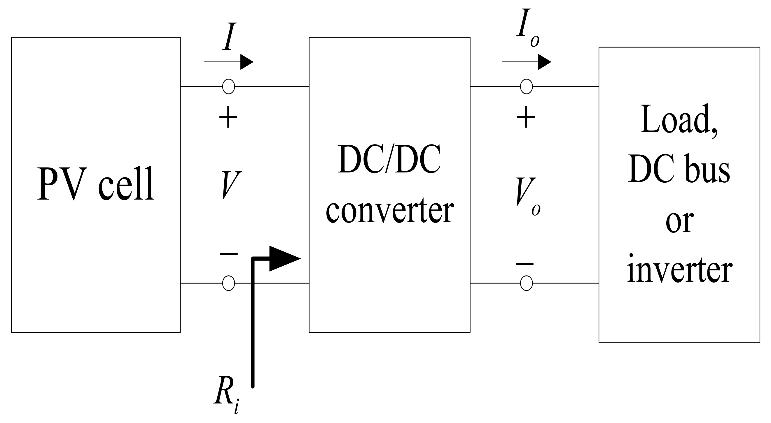
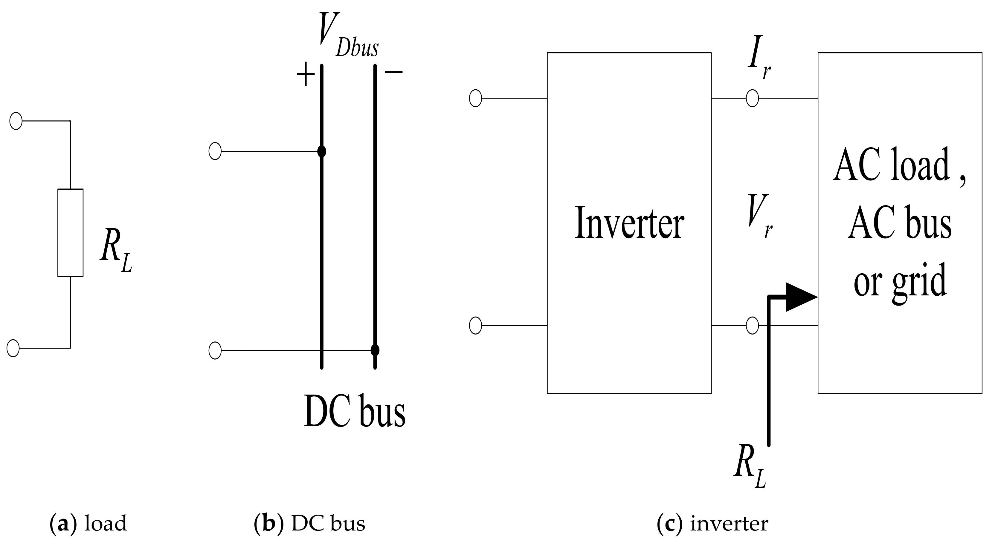
As is known to all, three basic DC/DC converters, i.e., the buck DC/DC converter, boost DC/DC converter, and buck/boost DC/DC converter, are usually used as the MPPT hardware circuits. They are usually united with a PV cell as the PV-buck system, PV-boost system, and PV-buck/boost system [20]. Meanwhile, the inverter (INV) is usually connected with them as PV-buck-INV system, PV-boost-INV system, and PV-buck/boost-INV system [21,22]. In addition, a DC bus (or battery) is usually connected with them as the PV-buck-DC system, PV-boost-DC system, and PV-buck/boost-DC system [17,23,24]. Here, the battery can be approximately regarded as a DC bus. However, there is no work to specially compare them from MPPT perspective. To fill in this gap, in this paper, these PV systems are selected as the research objects to analyze the influence of the system configuration to the CPR. In practical application, these results can be used as the theory foundation to select PV system with the fitting configuration.

This work is the first attempt to study the load range and DC bus range based on MPP-TCM. The innovations and contributions can be illustrated as follows:

(1).

The expressions of the CPR based on MPP-TCM under ideal conditions are first presented. They reveal the constraints between MPP-TCM and load resistance or bus voltage when the MPP of PV system always exists under ideal conditions.

(2).

These expressions in practical application are first proposed. Unlike ideal conditions, the nonlinear characteristics of the DC/DC converter and inverter are considered. Therefore, they provide the theoretical foundation for the use of the MPP-TCM in practical application.

(3).

The characteristics of the CPR changing with varying weather are shown. By these results, the CPR can be estimated by the data of irradiance and temperature in a certain area. Therefore, they supply an important theory basis for the hardware design, theoretical research, and product installation of PV systems.

(4).

The characteristics of the CPR changing with system configuration are disclosed. By these results, the area to guarantee the existence of the MPP can be estimated for PV systems with different configuration. Therefore, they are a good guide for the type selection, layout planning, and configuration design of PV systems.

The sections of this manuscript are arranged as follows. The expressions of the CPR under ideal conditions are proposed in Section 2. Based on them, the expressions of the CPR in practical application are proposed, and maximum and minimum values of the CPR are analyzed in Section 3. Some simulation experiments are performed to verify the accuracy of the theoretical analysis in Section 4. Finally, some discussions and conclusions are given in Section 5 and Section 6, respectively.

2. CPR under Ideal Conditions

2.1. Mathematical Modeling of PV System

The usual configuration of a PV system is shown by Figure 1. Here, the mathematical models of the PV cell can be expressed by Equations (1)–(3) [25]. Meanwhile, the buck, boost and buck/boost DC/DC converters can be expressed by Equations (4)–(6), respectively [26], where $I$ and $V$ represent the output current and voltage of PV cell, respectively. Obviously, they are also the input current and voltage of the DC/DC converter, respectively. $I_o$ and $V_o$ represent the output current and voltage of the DC/DC converter, respectively. $D$ represents the duty cycle of the pulse-width modulation (PWM) signal of the DC/DC converter. $I_{sc}$, $V_{oc}$, $I_m$, and $V_m$ represent the short circuit current, the open circuit voltage, the MPP current and voltage of PV cell at standard testing conditions (STC), respectively.

$$I=I_{sc}\left[1-C_1\left(e^{\frac{V}{C_2{V}_{oc}}}-1\right)\right]$$

(1)

$$C_1=\left(1-\frac{I_m}{I_{sc}}\right)e^{-\frac{V_m}{C_2{V}_{oc}}}$$

(2)

$$C_2=\frac{\frac{V_m}{V_{oc}}-1}{\mathit{ln}(1-\frac{I_m}{I_{sc}})}$$

(3)

$$V_o=DV$$

(4)

$$V_o=\frac{V}{1-D}$$

(5)

$$V_o=\frac{D}{1-D}V$$

(6)

In addition, the input resistance $R_i$ shown in Figure 1 can be expressed by Equation (7).

$$R_i=\frac{V}{I}$$

(7)

When the different output devices (shown in Figure 2) are connected with the DC/DC converter, there are the different equations of $R_i$, where $V_{Dbus}$ represents the voltage of the DC bus. $V_r$ and $I_r$ represent the root mean square (RMS) values of the output voltage and current of the inverter, respectively.

Firstly, assume a pure load resistance is connected with ideal buck DC/DC converter, boost DC/DC converter and buck/boost DC/DC converter, $R_i$ can be expressed by Equations (8)–(10), respectively.

$$R_i=\frac{R_L}{D^2}$$

(8)

$$R_i={(1-D)}^2{R}_L$$

(9)

$$R_i=\frac{{(1-D)}^2}{D^2}{R}_L$$

(10)

Secondly, when a DC bus is connected with the buck DC/DC converter, boost DC/DC converter, and buck/boost DC/DC converter, Equation (11) can be given.

$$V_o=V_{Dbus}$$

(11)

Thirdly, assuming an ideal inverter is connected with the DC/DC converter, Equations (12) and (13) can be satisfied.

$$V_r=\frac{V_{o}M}{\sqrt{2}}$$

(12)

$$V_o{I}_o=V_r{I}_r=\frac{V_r^2}{R_L}$$

(13)

Now, $R_i$ can be expressed by Equations (14)–(16) when the buck DC/DC converter, boost DC/DC converter and buck/boost DC/DC converter are used as the MPPT circuit, respectively.

$$R_i=\frac{2R_L}{M^2{D}^2}$$

(14)

$$R_i=\frac{2R_L{(1-D)}^2}{M^2}$$

(15)

$$R_i=\frac{2R_L{(1-D)}^2}{M^2{D}^2}$$

(16)

It is obvious that Equations (8)–(11) and (14)–(16) are some mathematical expressions based on input resistance under ideal conditions. They reveal some relationships between control signal ($D$ and $M$) and circuit parameters ($R_i$, $R_L$, and $V_{Dbus}$). By these relationships, the change range of $R_L$ and $V_{Dbus}$ can be studied to correctly use the linear equivalent model of PV cell.

2.2. Expressions of the CPR

According to Reference [19], when PV system is operating at its MPP, the four-parameter model of PV cell can be linearized as MPP-TCM and shown in Figure 3. In this case, the configuration of PV system can be replaced by Figure 4. Here $R_{sM}$ and $V_{sM}$ represent the internal resistance and open circuit voltage of MPP-TCM, respectively.

In order to find the expressions of the change range for two circuit parameters ($R_L$ and $V_{Dbus}$), firstly, Equations (17) and (18) can be given according to the maximum power transfer theorem under ideal conditions when a PV system is operating at the MPP.

$$R_{sM}=R_i$$

(17)

$$V=\frac{V_{sM}}{2}$$

(18)

When the output device is a load, Equations (19)–(21) can be given by submitting Equations (8)–(10) into Equation (17), respectively, where $D_{\max }$ represents the duty cycle of the PWM signal at the MPP.

$$D_{\max }=\sqrt{\frac{R_L}{R_{sM}}}$$

(19)

$$D_{\max }=1-\sqrt{\frac{R_{sM}}{R_L}}$$

(20)

$$D_{\max }=\frac{\sqrt{R_L}}{\sqrt{R_{sM}}+\sqrt{R_L}}$$

(21)

When the output device is a DC bus, Equations (22)–(24) can be given by submitting Equations (11) and (18) into Equations (4)–(6), respectively.

$$D_{\max }=\frac{2V_{Dbus}}{V_{sM}}$$

(22)

$$D_{\max }=1-\frac{V_{sM}}{2V_{Dbus}}$$

(23)

$$D_{\max }=\frac{2V_{Dbus}}{V_{sM}+2V_{Dbus}}$$

(24)

When the output device is an inverter, Equations (25)–(27) can be given by submitting Equations (14)–(17), respectively. Here $M$ represents the modulation ratio of the sine-wave pulse-width modulation (SPWM) signal of the inverter.

$$D_{\max }=\frac{1}{M}\sqrt{\frac{2R_L}{R_{sM}}}$$

(25)

$$D_{\max }=1-M\sqrt{\frac{R_{sM}}{2R_L}}$$

(26)

$$D_{\max }=\frac{\sqrt{2R_L}}{\sqrt{2R_L}+M\sqrt{R_{sM}}}$$

(27)

Secondly, the definition domain of $D_{\max }$ can be considered. As is known to all, Equation (28) must be satisfied when the MPP of PV system exists.

$$0\le D_{\max }\le 1$$

(28)

Submit Equations (19)–(21) into Equation (28), respectively, then Equations (29)–(31) can be given. They are the CPR of PV-buck system, PV-boost system, and PV-buck/boost system, respectively.

$$0<R_L\le R_{sM}$$

(29)

$$R_L\ge R_{sM}$$

(30)

$$R_L>0$$

(31)

Submit Equations (22)–(24) into Equation (28), respectively, then Equations (32)–(34) can be given. They are the CPR of PV-buck-DC system, PV-boost-DC system, and PV-buck/boost-DC system, respectively.

$$0<V_{Dbus}\le \frac{V_{sM}}{2}$$

(32)

$$V_{Dbus}\ge \frac{V_{sM}}{2}$$

(33)

$$V_{Dbus}>0$$

(34)

Submit Equations (25)–(27) into Equation (28), respectively, then Equations (35)–(37) can be given. They are the CPR of PV-buck-INV system, PV-boost-INV system, and PV-buck/boost-INV system, respectively.

$$0<R_L\le \frac{M^2{R}_{sM}}{2}$$

(35)

$$R_L\ge \frac{M^2{R}_{sM}}{2}$$

(36)

$$R_L>0$$

(37)

Finally, under ideal conditions, the expressions of the CPR can be given in

Table 1. CPR under ideal conditions.

Output Devices	Configuration	Expressions of the CPR
Load resistance	PV-buck	$0<R_L\le R_{sM}$
	PV-boost	$R_L\ge R_{sM}$
	PV-buck/boost	$R_L>0$
DC bus	PV-buck-DC	$0<V_{Dbus}\le 0.5V_{sM}$
	PV-boost-DC	$V_{Dbus}\ge 0.5V_{sM}$
	PV-buck/boost-DC	$V_{Dbus}>0$
Inverter	PV-buck-INV	$0<R_L\le 0.5M^2{R}_{sM}$
	PV-boost-INV	$R_L\ge 0.5M^2{R}_{sM}$
	PV-buck/boost-INV	$R_L>0$

for PV systems with different output devices. These expressions are the sufficient and necessary conditions to correctly use the MPP-TCM under ideal conditions. Certainly, they are also the sufficient and necessary conditions to track the MPP successfully under ideal conditions.

According to Table 1, it is obvious that $R_L$ is hardly constrained to track the MPP successfully for PV-buck/boost system and PV-buck/boost-INV system under ideal conditions because the MPP always exists. In other words, there always exists a value of $R_L$ to meet the conditions using the MPP-TCM regardless of PV-buck/boost system or PV-buck/boost-INV system under ideal conditions. Meanwhile, Table 1 also shows that there always exists a value of $V_{Dbus}$ to match the use of the MPP-TCM for PV-buck/boost-DC system under ideal conditions. By contrast, some constraints always exist for other PV systems, even if they are the ideal circuits according to Table 1.

In addition, by comparing Equation (29) with Equation (35) (or comparing Equation (30) with Equation (36)), it is obvious that the change ranges of the circuit parameter $R_L$ are influenced because of the used inverter. In other words, when the inverter is used, the change range of $R_L$ become narrower in PV system with the buck DC/DC converter while this range become wider in PV system with the boost DC/DC converter.

Obviously, the expressions shown in Table 1 reveal the constraints between circuit parameters and MPP-TCM when the MPP always exists under ideal conditions. In other words, only when the expressions are satisfied can the MPP-TCM be used correctly in the corresponding PV systems.

3. CPR in Practical Application

3.1. Expressions

In terms of practical application, because both DC/DC converter and inverter are non-ideal circuits, these expressions shown in Table 1 should be improved. It is generally known that the duty cycle cannot be too small for the buck DC/DC converter while it cannot be too big for the boost DC/DC converter. Meanwhile, for the buck/boost DC/DC converter, its duty cycle cannot be too small or too big. Therefore, to find the CPR in practical application, assume that the minimum duty cycle of the buck DC/DC converter or buck/boost DC/DC converter can be represented by $D_L$ and the maximum duty cycle of the boost DC/DC converter or buck/boost DC/DC converter can be represented by $D_U$. In this case, Equations (38)–(40) can be used for the buck DC/DC converter, boost DC/DC converter, and buck/boost DC/DC converter, respectively.

$$D_L\le D_{\max }\le 1$$

(38)

$$0\le D_{\max }\le D_U$$

(39)

$$D_L\le D_{\max }\le D_U$$

(40)

Firstly, for PV-buck system, PV-boost system, and PV-buck/boost system, submit Equations (19)–(21) into Equations (38)–(40), respectively, then Equations (41)–(43) can be presented. They are the CPR of PV systems with three DC/DC converters when the MPP-TCM is used.

$$D_L^2{R}_{sM}\le R_L\le R_{sM}$$

(41)

$$R_{sM}\le R_L\le \frac{R_{sM}}{{(1-D_U)}^2}$$

(42)

$$\frac{D_L^2{R}_{sM}}{{(1-D_L)}^2}\le R_L\le \frac{D_U^2{R}_{sM}}{{(1-D_U)}^2}$$

(43)

Secondly, for PV-buck-DC system, PV-boost-DC system, and PV-buck/boost-DC system, submit Equations (22)–(24) into Equations (38)–(40), respectively, then Equations (44)–(46) can be presented. They are the CPR of PV systems with three DC/DC converters and DC bus when the MPP-TCM is used.

$$\frac{D_L{V}_{sM}}{2}\le V_{Dbus}\le \frac{V_{sM}}{2}$$

(44)

$$\frac{V_{sM}}{2}\le V_{Dbus}\le \frac{V_{sM}}{2\left(1-D_U\right)}$$

(45)

$$\frac{D_L{V}_{sM}}{2\left(1-D_L\right)}\le V_{Dbus}\le \frac{D_U{V}_{sM}}{2\left(1-D_U\right)}$$

(46)

Thirdly, for PV-buck-INV system, PV-boost-INV system, and PV-buck/boost-INV system, submit Equations (25)–(27) into Equations (38)–(40), respectively, then Equations (47)–(49) can be presented. They are the CPR of PV systems with three DC/DC converters and inverter when the MPP-TCM is used

$$\frac{D_L^2{M}^2{R}_{sM}}{2}\le R_L\le \frac{M^2{R}_{sM}}{2}$$

(47)

$$\frac{M^2{R}_{sM}}{2}\le R_L\le \frac{M^2{R}_{sM}}{2{(1-D_U)}^2}$$

(48)

$$\frac{M^2{D}_L^2{R}_{sM}}{2{(1-D_L)}^2}\le R_L\le \frac{M^2{D}_U^2{R}_{sM}}{2{(1-D_U)}^2}$$

(49)

Finally, in practical application, the expressions of the CPR can be given in

Table 2. CPR in practical application.

Output Devices	Configuration	Expressions of the CPR
Load resistance	PV-buck	$D_L^2{R}_{sM}\le R_L\le R_{sM}$
	PV-boost	$R_{sM}\le R_L\le R_{sM}/{(1-D_U)}^2$
	PV-buck/boost	$D_L^2{R}_{sM}/{(1-D_L)}^2\le R_L\le D_U^2{R}_{sM}/{(1-D_U)}^2$
DC bus	PV-buck-DC	$0.5D_L{V}_{sM}\le V_{Dbus}\le 0.5V_{sM}$
	PV-boost-DC	$0.5V_{sM}\le V_{Dbus}\le 0.5V_{sM}/\left(1-D_U\right)$
	PV-buck/boost-DC	$0.5D_L{V}_{sM}/\left(1-D_L\right)\le V_{Dbus}\le 0.5D_U{V}_{sM}/\left(1-D_U\right)$
Inverter	PV-buck-INV	$0.5D_L^2{M}^2{R}_{sM}\le R_L\le 0.5M^2{R}_{sM}$
	PV-boost-INV	$0.5M^2{R}_{sM}\le R_L\le 0.5M^2{R}_{sM}/{(1-D_U)}^2$
	PV-buck/boost-INV	$0.5M^2{D}_L^2{R}_{sM}/{(1-D_L)}^2\le R_L\le 0.5M^2{D}_U^2{R}_{sM}/\left(1-D_U{)}^2\right]$

for PV systems with different output devices.

According to Equations (41)–(49), the CPR in practical application can be shown by Table 2. Comparing Table 2 with Table 1, it is obvious that the ranges of $R_L$ and $V_{Dbus}$ keep smaller. Meanwhile, unlike ideal conditions, there exist some constraints for PV-buck/boost system, PV-buck/boost-INV system, and PV-buck/boost-DC system in terms of practical application. In addition, Table 2 also shows that, when the inverter is used, the change range of $R_L$ becomes narrower in PV system with the buck DC/DC converter while it becomes wider in PV system with the boost DC/DC converter in practical application.

Obviously, the expressions shown in Table 2 illustrate the constraints between circuit parameters and MPP-TCM when the MPP always exists in practical application. Certainly, they disclose the inherent constraints among parameters when the MPP-TCM is used to linearize the overall PV system. In addition, they are also the sufficient and necessary conditions to guarantee the existence of the MPP in practical application.

3.2. Maximum and Minimum Values of the CPR

In practical application, the weather conditions usually keep varying with time and they can be represented by two main parameters ($S$ and $T$). To analyze the influence of the varying weather to the CPR, its maximum and minimum values under varying weather conditions should be studied. Here, assume that Equations (50) and (51) are satisfied for model parameters of the MPP-TCM, where $R_{sM\min }$ and $R_{sM\max }$ represent the minimum and maximum values of $R_{sM}$, respectively. Meanwhile, $V_{sM\min }$ and $V_{sM\max }$ represent the minimum and maximum values of $V_{sM}$, respectively.

$$R_{sM\min }\le R_{sM}\le R_{sM\max }$$

(50)

$$V_{sM\min }\le V_{sM}\le V_{sM\max }$$

(51)

Therefore, the maximum and minimum values of the CPR in practical application can be shown by

Table 3. Maximum and minimum values of the CPR.

Configuration	Maximum Ranges	Minimum Ranges
PV-buck	$D_L^2{R}_{sM\min }\le R_L\le R_{sM\max }$	$D_L^2{R}_{sM\max }\le R_L\le R_{sM\min }$
PV-boost	$R_{sM\min }\le R_L\le R_{sM\max }/{(1-D_U)}^2$	$R_{sM\max }\le R_L\le R_{sM\min }/{(1-D_U)}^2$
PV-buck/boost	$D_L^2{R}_{sM\min }/{(1-D_L)}^2\le R_L\le D_U^2{R}_{sM\max }/{(1-D_U)}^2$	$D_L^2{R}_{sM\max }/{(1-D_L)}^2\le R_L\le D_U^2{R}_{sM\min }/{(1-D_U)}^2$
PV-buck-DC	$0.5D_L{V}_{sM\min }\le V_{Dbus}\le 0.5V_{sM\max }$	$0.5D_L{V}_{sM\max }\le V_{Dbus}\le 0.5V_{sM\min }$
PV-boost-DC	$0.5V_{sM\min }\le V_{Dbus}\le 0.5V_{sM\max }/(1-D_U)$	$0.5V_{sM\max }\le V_{Dbus}\le 0.5V_{sM\min }/(1-D_U)$
PV-buck/boost-DC	$0.5D_L{V}_{sM\min }/(1-D_L)\le V_{Dbus}\le 0.5D_U{V}_{sM\max }/(1-D_U)]$	$0.5D_L{V}_{sM\max }/(1-D_L)\le V_{Dbus}\le 0.5D_U{V}_{sM\min }/(1-D_U)]$
PV-buck-INV	$0.5D_L^2{M}^2{R}_{sM\min }\le R_L\le 0.5M^2{R}_{sM\max }$	$0.5D_L^2{M}^2{R}_{sM\max }\le R_L\le 0.5M^2{R}_{sM\min }$
PV-boost-INV	$0.5M^2{R}_{sM\min }\le R_L\le 0.5M^2{R}_{sM\max }/{(1-D_U)}^2$	$0.5M^2{R}_{sM\max }\le R_L\le 0.5M^2{R}_{sM\min }/{(1-D_U)}^2$
PV-buck/boost-INV	$0.5M^2{D}_L^2{R}_{sM\min }/{(1-D_L)}^2\le R_L\le 0.5M^2{D}_U^2{R}_{sM\max }/{(1-D_U)}^2$	$0.5M^2{D}_L^2{R}_{sM\max }/{(1-D_L)}^2\le R_L\le 0.5M^2{D}_U^2{R}_{sM\min }/{(1-D_U)}^2$

. It is obvious that the maximum range of $R_L$ (or $V_{Dbus}$) is the necessary condition to use the linear cell model for every PV system. In other words, the maximum value of the CPR is the necessary condition of a successful MPPT control. By contrast, the minimum range of $R_L$ (or $V_{Dbus}$) is the sufficient condition to use the linear cell model for every PV system. In other words, the minimum range of the CPR is the necessary condition of a successful MPPT control.

Clearly, Table 1 and Table 2 show the sufficient and necessary conditions of using the linear cell model in PV systems while only some sufficient conditions or necessary conditions are given in Table 3. However, in practical application, these sufficient conditions or necessary conditions can usually play an important role in the hardware design, theoretical research, and product installation for PV system. On the one hand, because the boundaries of these sufficient and necessary conditions always vary with the weather parameters, it is very difficult to adjust whether the load (or bus voltage) of the operating system is varying within CPR in real time. For hardware designer, to make the MPP tracked successfully all the time, these sufficient conditions can be used to select the system configuration and circuit elements. For the theoretical researcher, these sufficient conditions can be used as the basis to guarantee the availability of the proposed control method. For system installers, these sufficient conditions can be used to estimate the MPPT effect according to the recorded data of solar irradiance and temperature in the installation area. On the other hand, the maximum selected value of the load (or bus voltage) can be reflected by these necessary conditions in practical application. It is obvious that these expressions can be used as a theoretical basis for the hardware design, theoretical research, and product installation of PV systems. In other words, for a PV system, if the selected value of its load (or bus voltage) is without the corresponding interval (“Maximum ranges” in Table 3), the MPP cannot be tracked successfully regardless of any MPPT methods. Certainly, in this case, the MPP-TCM cannot be used. In addition, when the MPP-TCM is used to study the overall linearization model of PV system, the results shown in Table 3 can provide the theoretical foundation.

4. Simulation Analysis

4.1. Accuracy of the Expressions

Some simulation experiments are done to test the accuracy of the expressions shown in Table 2. Here, assume that the values of $D_L$, $D_U$, and $M$ are 0.2, 0.8, and 0.8, respectively, in practical application. Meanwhile, assume all PV systems are operating at 5 different weather conditions shown in

Table 4. Operating conditions of PV system in simulations.

Operating Conditions	(a)	(b)	(c)	(d)	(e)
${}_S$ (${\mathrm{W}/\mathrm{m}}^2$)	1200	1000	800	600	500
${}_T$ ($°\mathrm{C}$)	45	35	25	20	20

. In all simulation experiments (including Section 4.2 and Section 4.3), the four cell parameters $I_{sc}$, $V_{oc}$, $I_m$, and $V_m$ are selected as 9.19 A, 22 V, 8.58 A, and 17.5 V at STC, respectively. In addition, although only the accuracy of the expressions shown in Table 2 are verified in this section, other results shown in Table 1 or Table 3 can also tested easily by analogy. Meanwhile, although only some operating conditions shown in Table 4 are used in these simulation experiments, other weather conditions can also be analyzed by analogy.

4.1.1. Test for Load Output Device

When the output device of PV system is a load resistance, some simulation experiments are performed, and the results are given by Figure 5, Figure 6 and Figure 7. Figure 5 shows the compared $D_{\max }$ curves varying with $R_L$ for PV-buck system under five operating conditions. Figure 6 show the compared $D_{\max }$ curves varying with $R_L$ for PV-boost system under 5 operating conditions. Figure 7 shows the compared $D_{\max }$ curves varying with $R_L$ for PV-buck/boost system under five operating conditions. Meanwhile, some main parameters in Table 2 are calculated and shown in

Table 5. Calculated values of some main parameters.

Operating Conditions		(a)	(b)	(c)	(d)	(e)
PV-buck system	$D_L^2{R}_{sM}$	0.0667	0.0807	0.1035	0.1408	0.1698
	$R_{sM}$	1.6669	2.0172	2.5879	3.5203	4.2450
PV-boost system	$R_{sM}$	1.6669	2.0172	2.5879	3.5203	4.2450
	$R_{sM}/{(1-D_U)}^2$	41.6732	50.4307	64.6963	88.0076	106.1255
PV-buck/boost system	$D_L^2{R}_{sM}/{(1-D_L)}^2$	0.1042	0.1261	0.1617	0.2200	0.2653
	$D_U^2{R}_{sM}/{(1-D_U)}^2$	26.6708	32.2757	41.4056	56.3249	67.9203

. They can be used as the compared objects to judge whether the simulation results shown in every zoom subgraph are accordant with conclusions given in Table 2.

Figure 5 shows that $D_{\max }$ keeps at 0.2 under $R_L<D_L^2{R}_{sM}$ condition while $D_{\max }$ remains at 1 under $R_L>R_{sM}$ condition for PV-buck system, which means that, in these cases, there is no MPP and the MPP-TCM cannot be used. Figure 6 shows that $D_{\max }$ remains at 0 under $R_L<R_{sM}$ condition while $D_{\max }$ remains at 0.8 under $R_L>R_{sM}/{(1-D_U)}^2$ condition for PV-boost system, which means that, in these cases, there is no MPP and the MPP-TCM cannot be used. Figure 7 shows that $D_{\max }$ keeps at 0.2 under $R_L<D_L^2{R}_{sM}/{(1-D_L)}^2$ condition while $D_{\max }$ remains at 0.8 under $R_L>D_U^2{R}_{sM}/{(1-D_U)}^2$ condition for PV-buck/boost system, which means that, in these cases, there is no MPP and the MPP-TCM cannot be used. By contrast, according to Figure 5, Figure 6 and Figure 7, $D_{\max }$ keeps varying with $R_L$ when $R_L$ is in its CPR (shown in Table 2), regardless of PV-buck system, PV-boost system, or PV-buck/boost system. In this case, the MPP always exists and the MPP-TCM can be used for these three PV systems.

In brief, the simulation results shown in Figure 5, Figure 6 and Figure 7 (including the zoom subgraph) are accordant with the corresponding data given in Table 5, although the $D_{\max }-R_L$ curves of PV systems are very different under different operating conditions. Therefore, a conclusion can be drawn that the expressions shown in Table 2 are accurate for PV-buck system, PV-boost system, and PV-buck/boost system.

4.1.2. Test for DC Bus Output Device

When the output device of PV system is a DC bus, some simulation experiments are performed, and the results are given by Figure 8, Figure 9 and Figure 10. Figure 8 shows the compared $D_{\max }$ curves varying with $V_{Dbus}$ for PV-buck-DC system under five operating conditions. Figure 9 show the compared $D_{\max }$ curves varying with $V_{Dbus}$ for PV-boost-DC system under 5 operating conditions. Figure 10 show the compared $D_{\max }$ curves varying with $V_{Dbus}$ for PV-buck/boost-DC system under five operating conditions. Meanwhile, some main parameters in Table 2 are calculated and shown in

Table 6. Calculated values of some main parameters.

Operating Conditions		(a)	(b)	(c)	(d)	(e)
PV-buck-DC system	$0.5D_L{V}_{sM}$	3.5331	3.4781	3.4825	3.5086	3.5258
	$0.5V_{sM}$	17.6654	17.3906	17.4126	17.5430	17.6288
PV-boost-DC system	$0.5V_{sM}$	17.6654	17.3906	17.4126	17.5430	17.6288
	$0.5V_{sM}/(1-D_U)$	88.3268	86.9529	87.0631	87.7149	88.1438
PV-buck/boost-DC system	$0.5D_L{V}_{sM}/(1-D_L)$	4.4163	4.3476	4.3531	4.3857	4.4072
	$0.5D_U{V}_{sM}/(1-D_U)$	70.6614	69.5623	69.6504	70.1719	70.5150

. They can also be used as the compared objects to judge whether the simulation results shown in every zoom subgraph are accordant with conclusions given in Table 2.

Figure 8 shows that $D_{\max }$ remains at 0.2 under $V_{Dbus}<0.5D_L{V}_{sM}$ condition while $D_{\max }$ remains at 1 under $V_{Dbus}>0.5V_{sM}$ condition for PV-buck-DC system, which means that, in these cases, there is no MPP and the MPP-TCM cannot be used. Figure 9 shows that $D_{\max }$ keeps at 0.2 under $V_{Dbus}<0.5V_{sM}$ condition while $D_{\max }$ keeps at 0.8 under $V_{Dbus}>0.5V_{sM}/(1-D_U)$ condition for PV-boost-DC system, which means that, in these cases, there is no MPP and the MPP-TCM cannot be used. Figure 10 shows that $D_{\max }$ keeps at 0.2 under $V_{Dbus}<0.5D_L{V}_{sM}/(1-D_L)$ condition while $D_{\max }$ remains at 0.8 under $V_{Dbus}>0.5D_U{V}_{sM}/(1-D_U)$ condition for PV-buck/boost-DC system, which means that, in these cases, there is no MPP and the MPP-TCM cannot be used. By contrast, according to Figure 8, Figure 9 and Figure 10, $D_{\max }$ keeps varying with $V_{Dbus}$ when $V_{Dbus}$ is in its CPR (shown in Table 2), regardless of PV-buck-DC system, PV-boost-DC system, or PV-buck/boost-DC system. In this case, there always exist the MPP and the MPP-TCM can be used for these three PV systems. In addition, Figure 8, Figure 9 and Figure 10 also show that the real-time values of $D_{\max }$ are hardly influenced by the different weather conditions. In addition, Figure 8, Figure 9 and Figure 10 also show that there is only a small difference among $D_{\max }-V_{Dbus}$ curves under five operating conditions. This means that, when $V_{Dbus}$ is given as a constant, there is a small difference for $D_{\max }$ even if the irradiance keeps greatly varying. For example, according to the zoom subgraphs, this difference of $D_{\max }$ is about 0.012 in Figure 8 while the values in Figure 9 and Figure 10 are about 0.003 and 0.004, respectively.

In brief, the simulation results shown in Figure 8, Figure 9 and Figure 10 (including the zoom subgraph) are accordant with the corresponding data given in Table 6. Therefore, a conclusion can be drawn that the expressions shown in Table 2 are accurate for PV-buck-DC system, PV-boost-DC system, and PV-buck/boost-DC system.

4.1.3. Test for Inverter Output Device

When the output device of PV system is an inverter, some simulation experiments are performed, and the results are given by Figure 11, Figure 12 and Figure 13. Figure 11 show the compared $D_{\max }$ curves varying with $R_L$ for PV-buck-INV system under five operating conditions. Figure 12 show the compared $D_{\max }$ curves varying with $R_L$ for PV-boost-INV system under five operating conditions. Figure 13 shows the compared $D_{\max }$ curves varying with $R_L$ for PV-buck/boost-INV system under five operating conditions. Meanwhile, some main parameters in Table 2 are calculated and shown in

Table 7. Calculated values of some main parameters.

Operating Conditions		(a)	(b)	(c)	(d)	(e)
PV-buck-INV system	$0.5D_L^2{M}^2{R}_{sM}$	0.0213	0.0258	0.0331	0.0451	0.0543
	$0.5M^2{R}_{sM}$	0.5334	0.6455	0.8281	1.1265	1.3584
PV-boost-INV system	$0.5M^2{R}_{sM}$	0.5334	0.6455	0.8281	1.1265	1.3584
	$0.5M^2{R}_{sM}/{(1-D_U)}^2$	13.3354	16.1378	20.7028	28.1624	33.9602
PV-buck/boost-INV system	$0.5M^2{D}_L^2{R}_{sM}/{(1-D_L)}^2$	0.0333	0.0403	0.0518	0.0704	0.0849
	$0.5M^2{D}_U^2{R}_{sM}/{(1-D_U)}^2$	8.5347	10.3282	13.2498	18.0240	21.7345

. They can also be used as the compared objects to judge whether the simulation results shown in every zoom subgraph are accordant with conclusions given in Table 2.

Figure 11 show that $D_{\max }$ remains at 0.2 under $R_L<0.5M^2{D}_L^2{R}_{sM}$ condition while $D_{\max }$ remains at 1 under $R_L>0.5M^2{R}_{sM}$ condition for PV-buck-INV system, which means that, in these cases, there is no MPP and the MPP-TCM cannot be used. Figure 12 shows that $D_{\max }$ keeps at 0 under $R_L<0.5M^2{R}_{sM}$ condition while $D_{\max }$ remains at 0.8 under $R_L>0.5M^2{R}_{sM}/{(1-D_U)}^2$ condition for PV-boost-INV system, which means that, in these cases, there is no MPP and the MPP-TCM cannot be used. Figure 13 show that $D_{\max }$ remains at 0.2 under $R_L<0.5M^2{D}_L^2{R}_{sM}/{(1-D_L)}^2$ condition while $D_{\max }$ keeps at 0.8 under $R_L>0.5M^2{D}_U^2{R}_{sM}/{(1-D_U)}^2$ condition for PV-buck/boost-INV system, which means that, in these cases, there is no MPP and the MPP-TCM cannot be used. By contrast, according to Figure 11, Figure 12 and Figure 13, $D_{\max }$ keeps varying with $R_L$ when $R_L$ is in its CPR (shown in Table 2) regardless of PV-buck-INV system, PV-boost-INV system, or PV-buck/boost-INV system. In this case, the MPP always exists and the MPP-TCM can be used for these three PV systems.

In brief, the simulation results shown in Figure 11, Figure 12 and Figure 13 (including the zoom subgraph) are accordant with the corresponding data given in Table 7, although the $D_{\max }-R_L$ curves are very different under different operating conditions. Therefore, a conclusion can be drawn that the expressions shown in Table 2 are accurate for PV-buck-INV system, PV-boost-INV system or PV-buck/boost-INV system.

All in all, a conclusion can be drawn that the expressions shown in Table 2 are accurate in terms of practical application.

4.2. Characteristics of the CPR Changing with the Varying Weather

According to Table 2 and Table 3, two key parameters to express the boundaries of the CPR are $R_{sM}$ and $V_{sM}$. However, they keep varying with time, which leads to the uncertainty of CPR. Therefore, to analyze their characteristics changing with $S$ and $T$, some simulation experiments are performed, and simulation results can be shown by Figure 14 and Figure 15.

Figure 14a shows that the relationship between $V_{sM}$ and $S$ is an approximate parabolic curve when $T$ keeps constant. The minimum value of $V_{sM}$ is reached when $S$ is about 638.25 ${\mathrm{W}/\mathrm{m}}^2$. Figure 14b shows that $V_{sM}$ is the linear decreasing function of $T$ when $S$ remains unchanged. Figure 14c shows the characteristics of $V_{sM}$ when both $S$ and $T$ are varying. Here, a function $V_{sM}(S,T)$ can be used to describe the parameter $V_{sM}$. Its maximum value ($V_{sM\max }$) and minimum value ($V_{sM\min }$) can be represented by Equations (52) and (53), respectively.

$$V_{sM\max }=\left\{\begin{array}{c}{V}_{sM}(S_{\min },T_{\min })\\ V_{sM}(S_{\max },T_{\min })\end{array}\right.\begin{array}{c},\\ ,\end{array}\begin{array}{c}\forall S\le 638.25 \mathrm{or} S_{\min }+S_{\max }\le 1276.5\\ \forall S\ge 638.25 \mathrm{or} S_{\min }+S_{\max }\ge 1276.5\end{array}$$

(52)

$$V_{sM\min }=\left\{\begin{array}{l}{V}_{sM}(S_{\max },T_{\max })\hfill \\ V_{sM}(638.25,T_{\max })\hfill \\ V_{sM}(S_{\min },T_{\max })\hfill \end{array}\right.\begin{array}{c},\\ ,\\ ,\end{array}\begin{array}{l}\forall S<638.25\hfill \\ \mathrm{others}\hfill \\ \forall S>638.25\hfill \end{array}$$

(53)

Figure 15a shows that $R_{sM}$ is the monotone decreasing function of $S$ when $T$ keeps constant. Meanwhile, Figure 15b shows that $R_{sM}$ is the linear decreasing function of $T$ when $S$ remains unchanged. Figure 15c shows the characteristics of $R_{sM}$ when both $S$ and $T$ are varying. Here, a function $R_{SM}(S,T)$ can be used to describe the parameter $R_{sM}$. Its maximum value ($R_{sM\max }$) and minimum value ($R_{sM\min }$) can be expressed by Equations (54) and (55), respectively.

$$R_{sM\max }=R_{sM}(S_{\min },T_{\min })$$

(54)

$$R_{sM\min }=R_{sM}(S_{\max },T_{\max })$$

(55)

According to Equations (52)–(55), on the one hand, the CPR shown in Table 3 can be calculated after the parameters $S_{\max }$, $S_{\min }$, $T_{\max }$, and $T_{\min }$ in a certain area are obtained. In terms of practical application, it is beneficial to the hardware design, theoretical research, and product installation of a PV system. On the other hand, these results reveal how these CPR are influenced by the varying weather. Obviously, it is beneficial for the planning, layout, and design of a PV system.

In a word, the CPR will change with $S$ and $T$.

4.3. Comparison of the CPR for Different PV Systems

In practical application, there are a lot of PV systems for our choice. Therefore, it is very necessary to compare their CPR. Here, assume that the values of $D_L$, $D_U$, and $M$ are the same as Section 4.1. In this case, Table 2 can be replaced by

Table 8. Calculated values of the CPR.

Outputs	Configuration	CPR
Load resistance	PV-buck	$0.04R_{sM}\le R_L\le R_{sM}$
	PV-boost	$R_{sM}\le R_L\le 25R_{sM}$
	PV-buck/boost	$0.0625R_{sM}\le R_L\le 16R_{sM}$
DC bus	PV-buck-DC	$0.1V_{sM}\le V_{Dbus}\le 0.5V_{sM}$
	PV-boost-DC	$0.5V_{sM}\le V_{Dbus}\le 2.5V_{sM}$
	PV-buck/boost-DC	$0.125V_{sM}\le V_{Dbus}\le 2V_{sM}$
Inverter	PV-buck-INV	$0.0128R_{sM}\le R_L\le 0.32R_{sM}$
	PV-boost-INV	$0.32R_{sM}\le R_L\le 8R_{sM}$
	PV-buck/boost-INV	$0.02R_{sM}\le R_L\le 5.12R_{sM}$

.

According to Table 8, for PV systems with different output devices, the load range can be shown by Figure 16 and the bus-voltage range can be shown by Figure 17. In Figure 16, A area shaded by red lines represents the load range where the MPP always exists if the PV-boost system or PV-boost-INV system is used. By contrast, B area shaded by blue lines represents the load range where the MPP always exists if the PV-buck system or PV-buck-INV system is used. In Figure 17, D area shaded by red lines represents the range of the bus voltage where the MPP always exists if the PV-boost-DC system is used. By contrast, E area shaded by blue lines represents the range of the bus voltage where the MPP always exists if the PV-buck-DC system is used. Obviously, in these areas, the existence of the MPP implies the usability of the MPP-TCM. In addition, according to Table 8, the values of $\alpha$, $\beta$, $\delta$, $\zeta$, $\xi$, and $\upsilon$ can be shown by

Table 9. Parameter values corresponding to Figure 16 and Figure 17.

PV Systems	$\mathit{\alpha }$	$\mathit{\beta }$	$\mathit{\delta }$	PV Systems	$\mathit{\zeta }$	$\mathit{\xi }$	$\mathit{\upsilon }$
PV-buck	/	0.04	1	PV-buck-DC	/	0.1	0.5
PV-boost	25	/	1	PV-boost-DC	2.5	/	0.5
PV-buck/boost	16	0.0625	1	PV-buck/boost-DC	2	0.125	0.5
PV-buck-INV	/	0.0128	0.32
PV-boost-INV	8	/	0.32
PV-buck/boost-INV	5.12	0.02	0.32

.

For PV-buck/boost system and PV-buck/boost-INV system, their load ranges can be still expressed by Figure 16. Unlike PV-buck system, PV-boost system, PV-buck-INV system and PV-boost-INV system, their MPP always exist in both A area and B area. In A area, the buck/boost DC/DC converter works in the “boost” mode while its “buck” mode is implemented in B area. Meanwhile, for PV-buck/boost-DC system, their bus-voltage ranges can be still expressed by Figure 17. Unlike PV-buck-DC system and PV-boost-DC system, their MPP always exist in both D area and E area. In D area, the buck/boost DC/DC converter works in the “boost” mode while its “buck” mode is implemented in E area.

Some simulation experiments are also undertaken to further analyze the CPR. The simulation results are shown by Figure 18, Figure 19, Figure 20, Figure 21, Figure 22 and Figure 23. In Figure 18, ${\mathrm{UB}}_{\mathrm{PVbuck}}$, ${\mathrm{LB}}_{\mathrm{PVbuck}}$, ${\mathrm{UB}}_{\mathrm{PVbuckINV}}$, and ${\mathrm{LB}}_{\mathrm{PVbuckINV}}$ represent the upper boundary of the load range for PV-buck system, lower boundary of the load range for PV-buck system, upper boundary of the load range for PV-buck-INV system, and lower boundary of the load range for PV-buck-INV system, respectively. By analogy, other boundaries are also represented in Figure 18, Figure 19, Figure 20, Figure 21, Figure 22 and Figure 23. In addition, some zoom subgraphs are given in Figure 18, Figure 19 and Figure 20 to show the numerical values of these boundaries more clearly.

According to Figure 18, Figure 19, Figure 20, Figure 21, Figure 22 and Figure 23 and Table 8 and Table 9, some conclusions can be drawn. Firstly, when the boost DC/DC converter is used as the MPPT circuit, the load range or bus-voltage range is much wider than buck DC/DC converter. Secondly, when the buck/boost DC/DC converter is used as the MPPT circuit, there is the widest load range or bus-voltage range. Thirdly, because both $R_{sM}$ and $V_{sM}$ are the function of $S$ and $T$, the width of the load range or bus-voltage range will change with $S$ and $T$. Fourthly, when the inverter is used, the change range of $R_L$ become narrower in PV system with the buck DC/DC converter while this range become wider in PV system with the boost DC/DC converter in practical application. In addition, Figure 18, Figure 19, Figure 20, Figure 21, Figure 22 and Figure 23 are actually the concretion of Figure 16 and Figure 17. Therefore, by these figures (especially by the zoom subgraphs) not only the change range of $R_L$ is shown, but the accuracy of the numerical values of the boundaries given in Table 8 and Table 9 is also verified.

In a word, not only the use of the inverter, but also the different choice of the DC/DC converter maybe lead to the change of the CPR.

5. Discussions

In this work, the expressions in Table 1 are proposed under ideal DC/DC converter and inverter conditions. By contrast, the change range of the control signal of the DC/DC converter and inverter is considered to improve these results, just as Table 2 shows. However, in terms of practical application, the MPPT control of PV system is usually influenced by some other factors, such as the installed PV power, the nonideal DC/DC converter, the nonideal inverter, the transmission efficiency and so on. Therefore, the expressions shown in Table 1, Table 2 and Table 3 will be influenced by them in a certain extent. However, these factors can be ignored. There are some reasons for this, as follows. On the one hand, the theoretical research need be greatly simplified by using the ideal DC/DC converter and inverter, just as other works have been doing. On the other hand, the emphasis of this work is to disclose the constraints between MPP-TCM and load resistance or bus voltage when the MPP of PV system always exists. Obviously, the harvest of these relationships is very beneficial to study the MPPT control method with MPP-TCM. Finally, the expressions shown in Table 1, Table 2 and Table 3 represent the key results. Based on them, in practical application, other factors can be easily considered and involved.

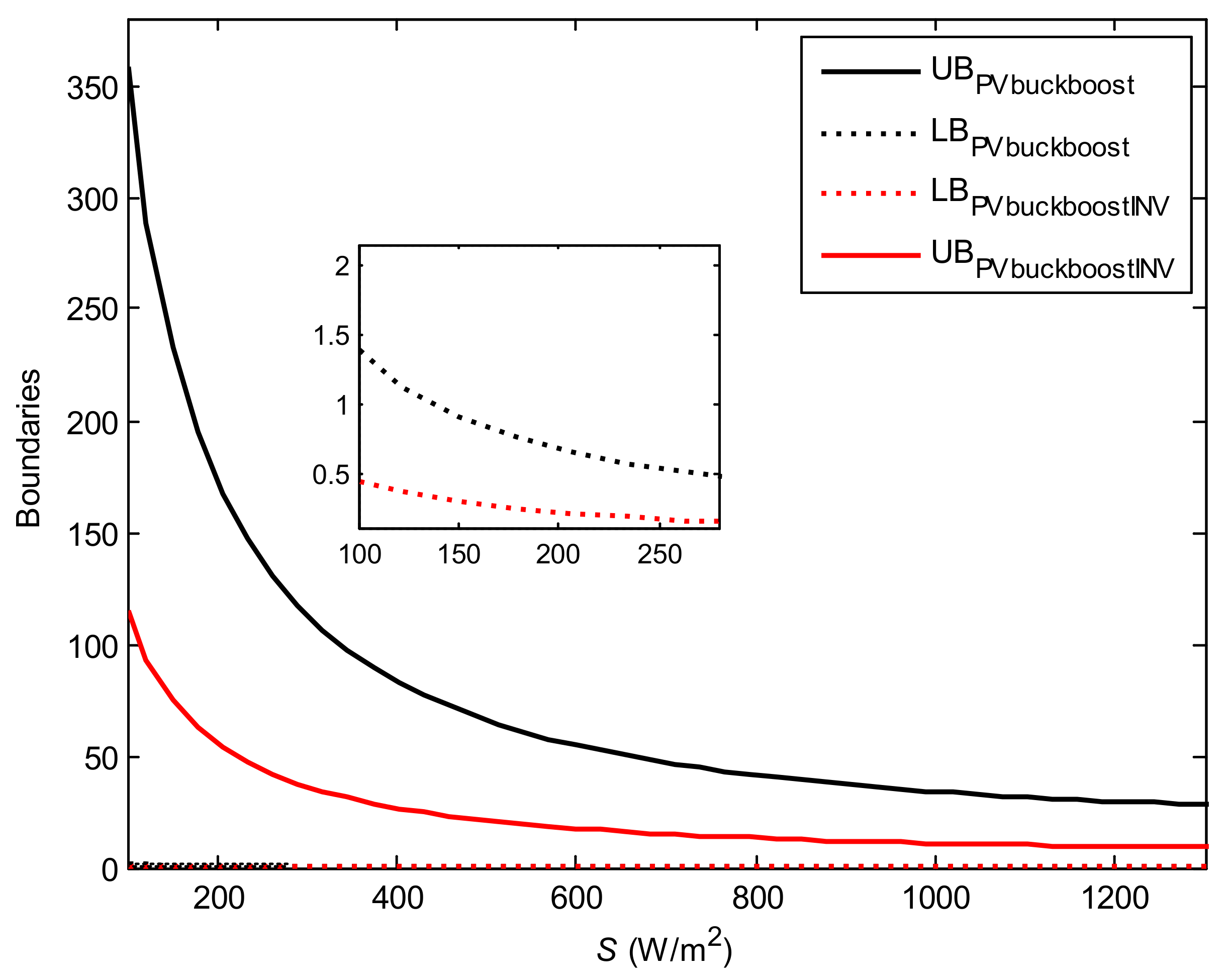
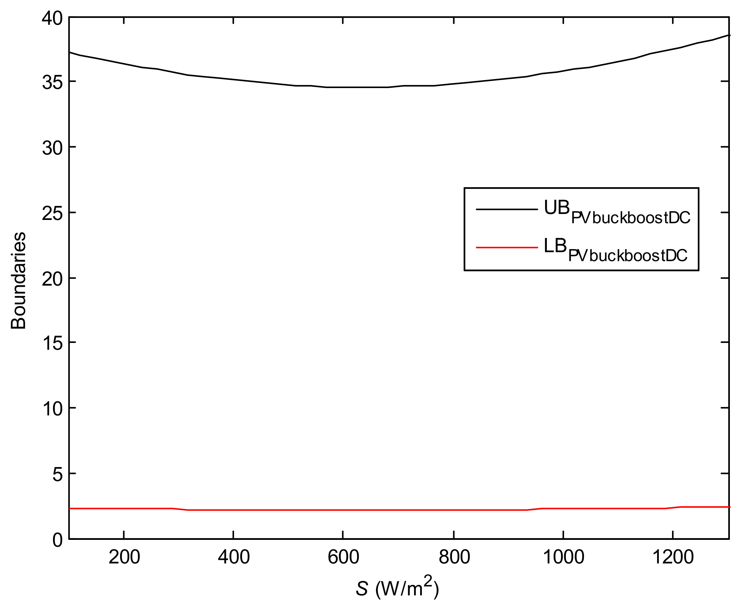
In practical application, $R_L$ can be estimated and calculated by Equations (56)–(61) for PV-buck system [10], PV-boost system, PV-buck/boost system, PV-buck-INV system, PV-boost-INV system and PV-buck/boost-INV system, respectively. Here, $C$ and $P_{o\max }$ can be approximately calculated by Equations (62) and (63), respectively [19].

$$R_L=\frac{C^2{D}_{\max }^2}{P_{o\max }}$$

(56)

$$R_L=\frac{C^2}{P_{o\max }{(1-D_{\max })}^2}$$

(57)

$$R_L=\frac{C^2{D}_{\max }^2}{P_{o\max }{(1-D_{\max })}^2}$$

(58)

$$R_L=\frac{M^2{C}^2{D}_{\max }^2}{2P_{o\max }}$$

(59)

$$R_L=\frac{M^2{C}^2}{2{(1-D_{\max })}^2{P}_{o\max }}$$

(60)

$$R_L=\frac{M^2{C}^2{D}_{\max }^2}{2{(1-D_{\max })}^2{P}_{o\max }}$$

(61)

$$C=4.62\times {10}^{-6}\times {(S-638.25)}^2+17.287+(25-T)\times 0.0516$$

(62)

$$P_{o\max }=\left\{\begin{array}{l}2.943\times {10}^{-8}{S}^3-2.992\times {10}^{-5}{S}^2+0.1497S+2.664-0.045T\hfill \\ 2.943\times {10}^{-8}{S}^3-2.992\times {10}^{-5}{S}^2+0.1497S+2.664\hfill \end{array}\right.\begin{array}{cc}& 0\le T\le 40\\ & -20\le T\le 0\end{array}$$

(63)

In addition, the voltage level of $V_r$ in Section 4.1.3 can be estimated under $V=V_{oc}$, $D_{\max }=0.8$ and $M=0.8$ conditions for PV-boost-INV and PV-buck/boost-INV systems. Meanwhile, it can be also estimated under $V=V_{oc}$, $D_{\max }=1$ and $M=0.8$ conditions for PV-buck-INV system.

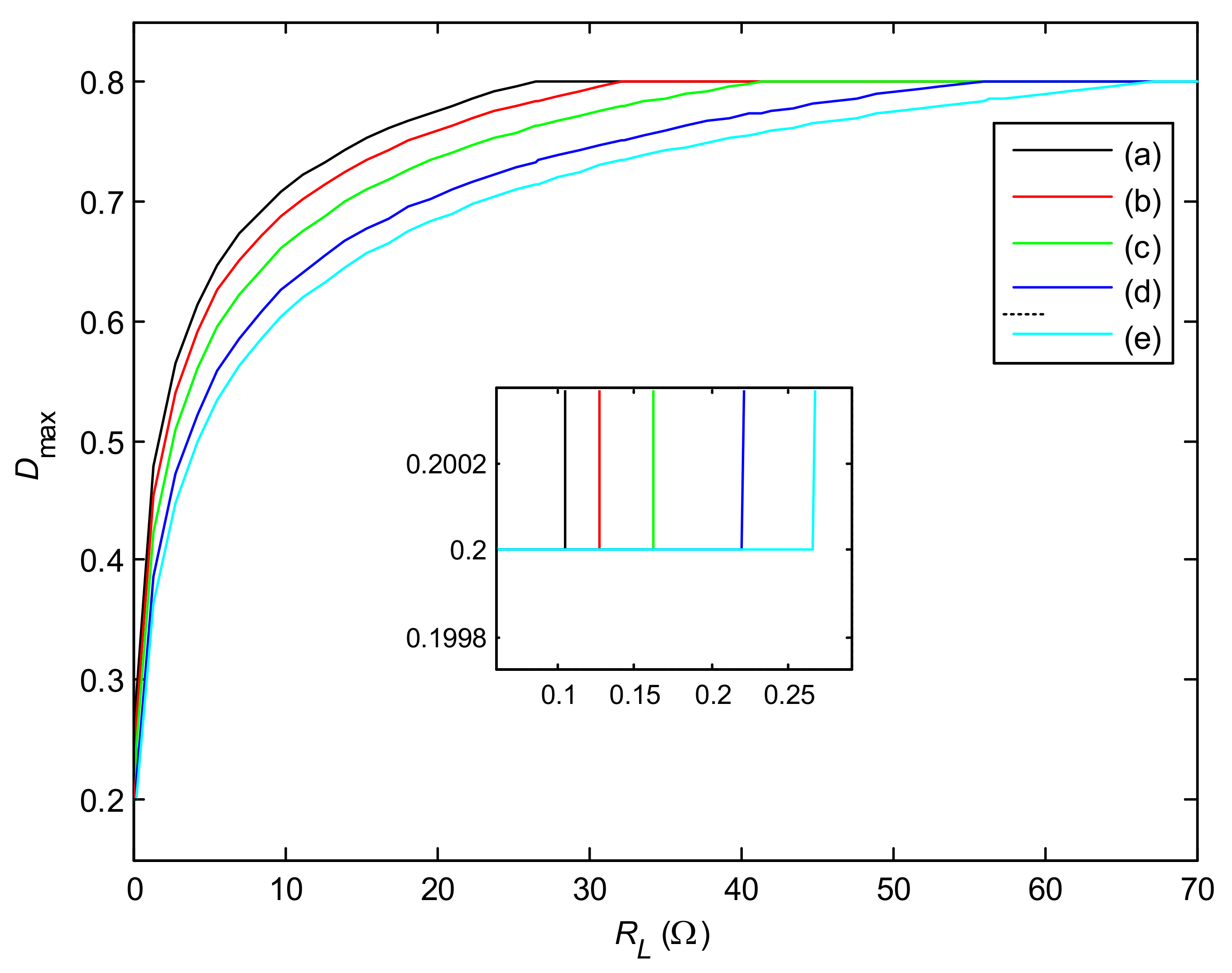
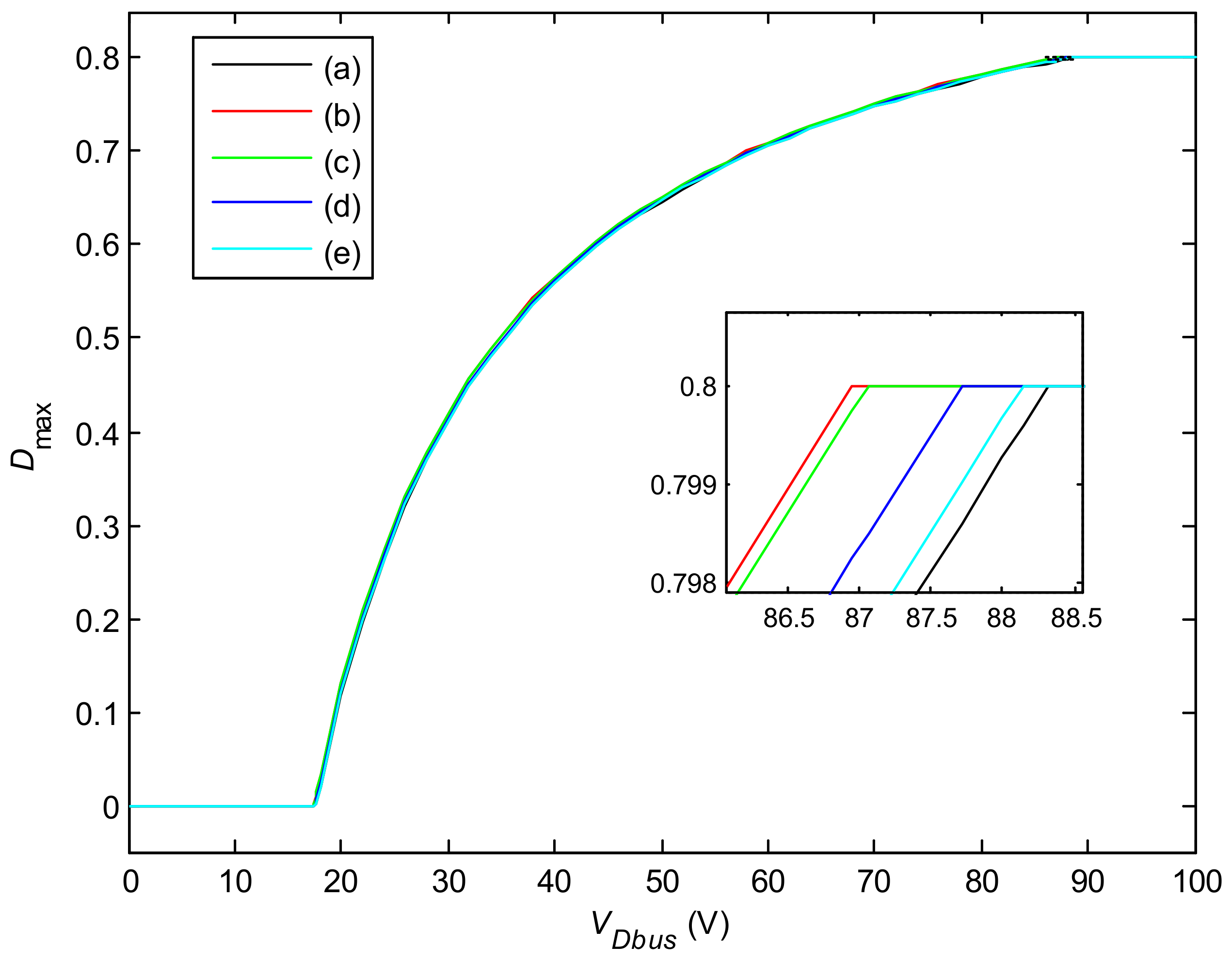
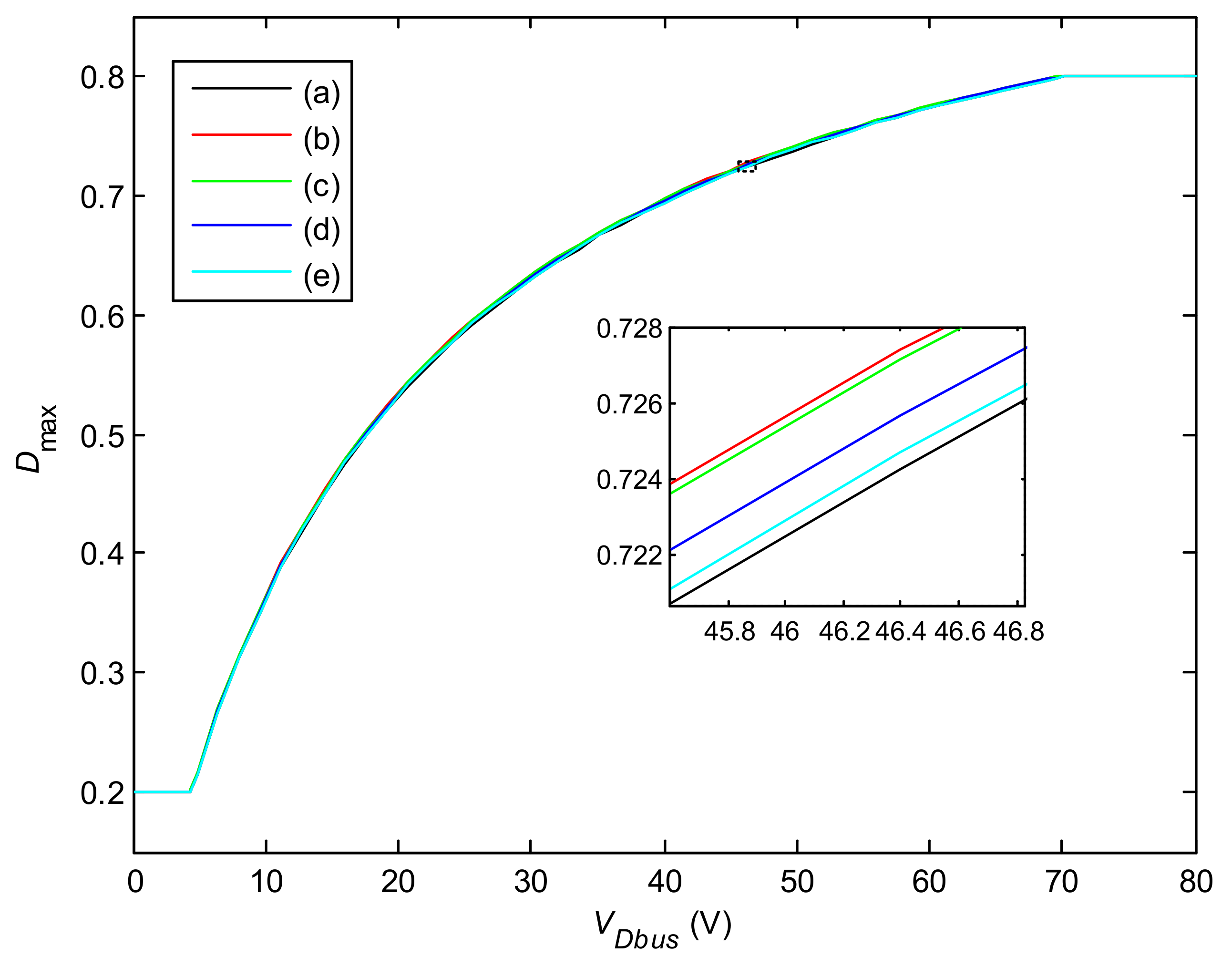
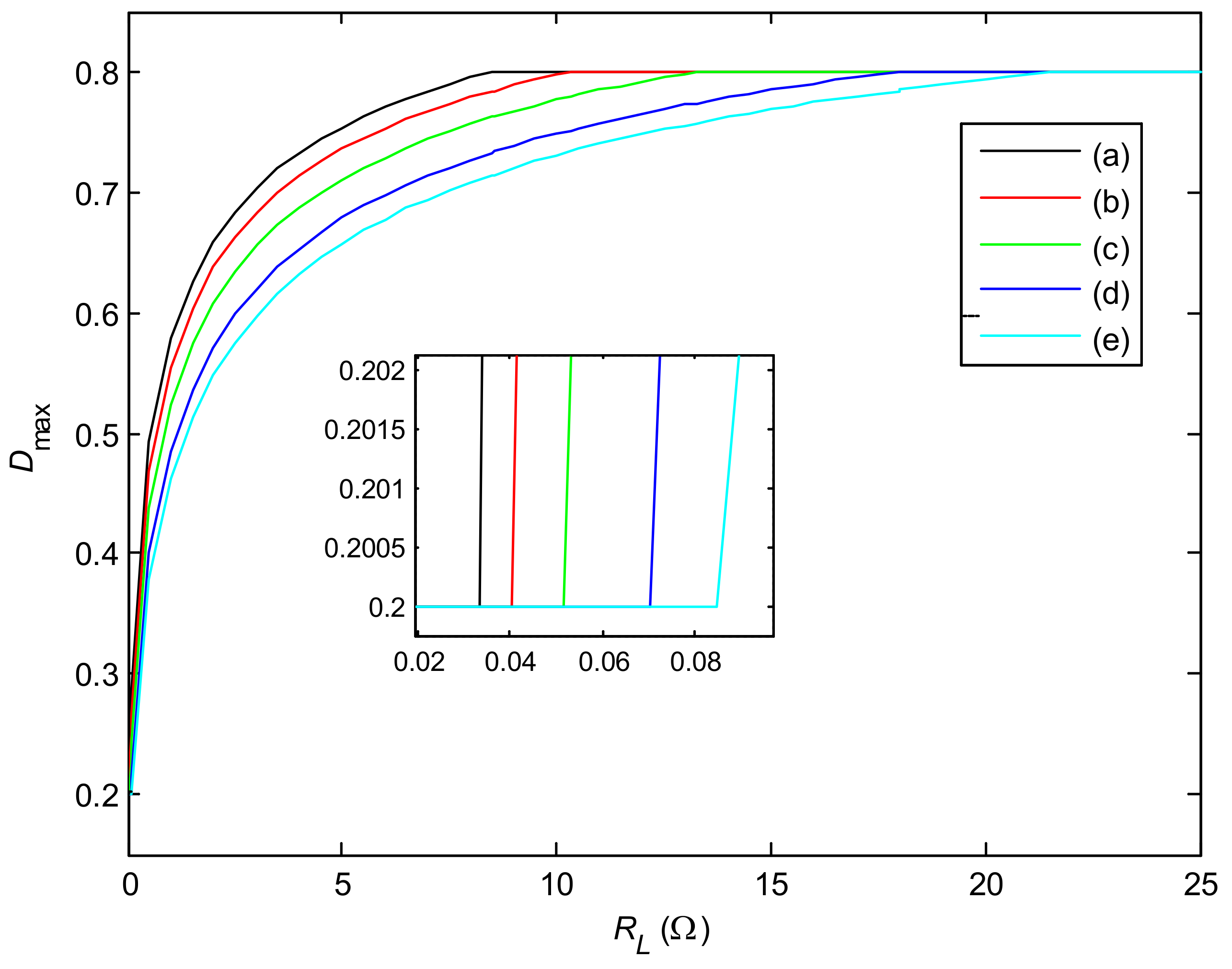
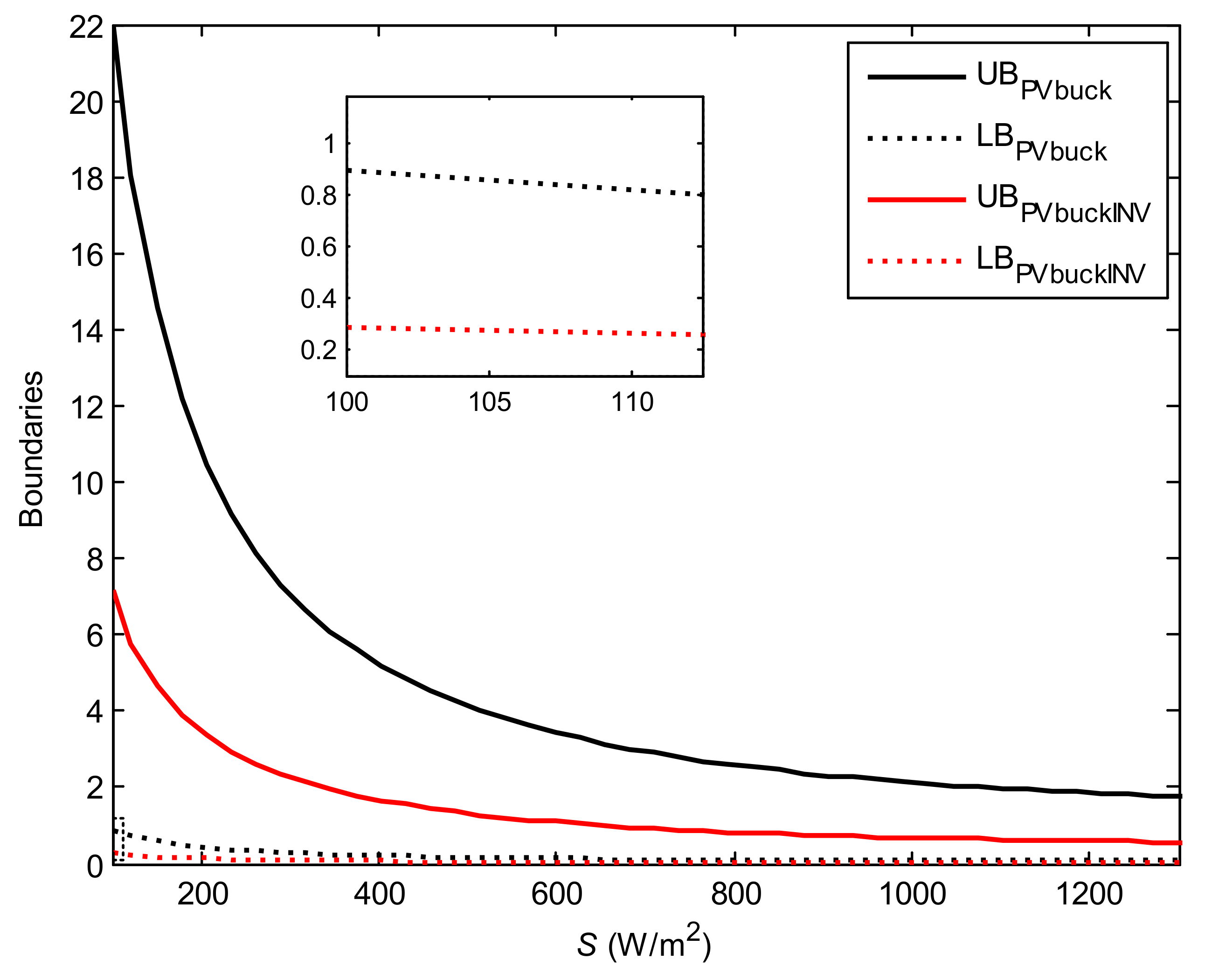
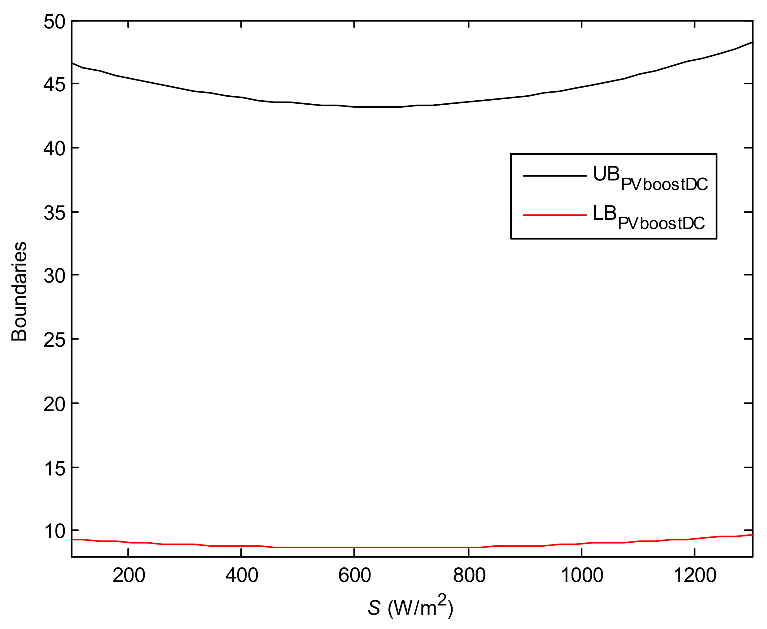
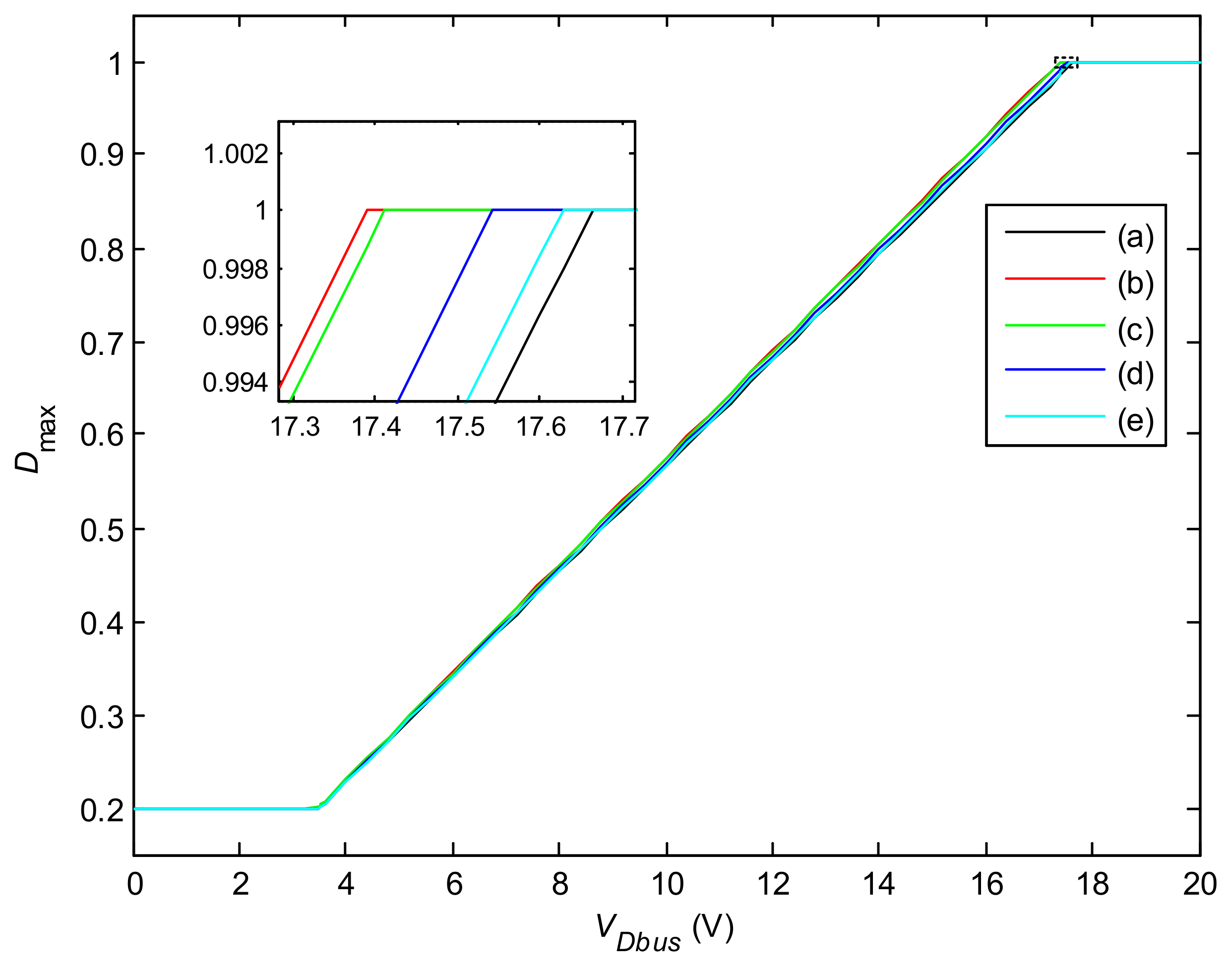
According to

Table 10. $V_r$ under operating conditions given in Table 4.

PV Systems	Parameters	(a)	(b)	(c)	(d)	(e)
PV-buck-INV	Maximum limit value of $V_r$ (V)	12.278	12.087	12.102	12.193	12.252
PV-boost-INV	Maximum limit value of $V_r$ (V)	61.388	60.433	60.510	60.963	61.261
PV-buck/boost-INV	Maximum limit value of $V_r$ (V)	49.111	48.347	48.408	48.770	49.009

, the voltage levels of $V_r$ considered for the results in Figure 11, Figure 12 and Figure 13 are less than 12.3 V, 61.5 V, and 49.5 V, respectively. Although these results have been presented at a lower voltage level, other levels can be easily analyzed by analogy. Therefore, the verification of the results shown in Table 2 is not influenced by the voltage level of $V_r$.

6. Conclusions

In this paper, for PV systems with three different outputs, the expressions of their CPR have been proposed under ideal conditions and in practical application, respectively. Meanwhile, the characteristics of the CPR have been analyzed under varying weather and different system configuration conditions. Finally, some simulation experiments verify the accuracy of the expressions of the CPR. Meanwhile, simulation results also show that not only are these CPR influenced by the varying $S$ and $T$, but the use of the inverter or the different choice of the DC/DC converter may also lead to the change of the CPR. In this work, the difficult question concerning when the MPP-TCM can be used is thoroughly solved, which plays an important role in studying the overall linearization of PV systems.

Future work on the subject will be focused on the use of the CPR to propose the overall linear model of PV system. To realize this purpose, on the one hand, these results on the CPR will be considered as one of the bridges to connect the inputs with outputs. On the other hand, some main factors in practical application should be taken in account. For example, how the CPR is influenced by the transmission efficiency should be analyzed.