1. Introduction
Energy consumption for transportation systems, especially freight transport, is growing. This is in addition to increasing urbanization trends and economic development of cities. The International Energy Agency (IEA) estimates that transportation energy consumption will increase by nearly 40% between 2018 and 2050 [
1]. A major part of urban freight is carried out by trucks and vans, which causes problems, such as increasing fossil fuel consumption, greenhouse gas emission (GHG), traffic congestion, and noise pollution. In order to have more sustainable cities, logistics companies should be encouraged to shift from road to rail. The European Commission (EC) consistently provides public funding to promote the shift of freight traffic from road to rail [
2,
3,
4]. However, rail’s share in the European freight and passenger transport markets is still not satisfactory. Utilizing urban railways to distribute urban freight can be a sustainable solution (some cities across the world have already put this into practice). For instance, in Zurich, in 2004, a project that involved collecting waste was carried out via 94 trips of a cargo tram system, which reduced 5020 km in regards to road commercial transport. The system caused decreases in CO
2 (4911.3 kg), SO
2 (1.4 kg), NO
x (80.6 kg), PM10 (2.3 kg), VOC (4.2 kg) emissions, the consumption of diesel fuel (37,500 L), and 960 h of truck operations [
5].
The main idea of the freight tram involves using existing tramlines to deliver goods from logistics centers of companies to micro depots instead of lorries. This study aimed to identify, initially, the possible routes, and to find the best route, by comparing the alternatives according to energy consumption. We created different paths from the logistics hubs to micro depots for each scenario using Google Earth Pro software. As a consumption calculation method, we suggested splitting the routes into the sections at which the tram must brake Each section used the Davis formula; the following was estimated: driving resistance, tractive force, and energy consumption. To estimate the tram trajectory (instantaneous acceleration, velocity, and distance), we used the onboard method via a simple GPS mobile application that recorded instantaneous accelerations.
1.1. Literature Review
The main applications (among European cities) that can be referred to are: Cargo Tram in Dresden, City Cargo of Amsterdam, GüterBim in Vienna, Cargo tram in Zurich, Monoprix in Paris, Logistiktram in Frankfurt, and the freight tram scheme in Barcelona [
6,
7]. However, only the projects in Dresden, Zurich, and Paris are still in operation. The analysis of the success and failure factors of the freight tram projects can be found in [
8]. Although rail vehicles (compared to road vehicles) have more weight and volume capacity, the main problems of using rail in urban freight are low accessibility, limited flexibility, sharing line capacity with passenger service, and high system costs [
9]. The creation of micro depots, with multipurpose uses or urban consolidation centers, in crowded city centers, leads to the reduction of urban rail weaknesses, such as accessibility, flexibility, and limited line capacity. Reduction of commercial vehicle movements in the urban area, more possibility of emission-free vehicle (such as cargo bikes and electric vehicles) use for the “last mile delivery”, more efficient operations of urban freight transport, and less need for logistics storages and activities, are the main advantages of a joint depot [
10]. In urban areas, the main issues of the environment, customers, and logistics suppliers are related to the last mile delivery. Therefore, the integration of urban freight alternatives and environment-friendly strategies is a critical aspect of urban transport planning [
11]. The performed study in [
12] modeled the combination of passenger and freight flow in the last mile delivery. In [
13], the related articles that were published from 2013 to 2018 to define sustainable inner-urban intermodal transportation in freight distribution were comprehensively reviewed.
To use available rail infrastructure, or construct new infrastructure to transport urban freight, a socioeconomic scheme should be defined. The scheme must estimate both the operational and environmental costs and benefits [
14]. A viability study from a business–economic and a socioeconomic perspective for a freight tram system was presented in [
15]. To decrease the related costs of the rail system, we considered energy consumption as one of the important key indicators for routing a tramline, and in scenario comparisons, as well as the shortest path, service demand, traffic congestion, and delay. This paper also assesses environmental effects in terms of road vehicle mileage and related emission reduction.
1.2. Paper Contribution
The paper carried out an in-depth study, mainly focusing on the effects of strategies for urban sustainability, using urban rail systems on the settlement confirmation of the analyzed case study. Data collections were performed primarily via literature and project reviews, interviews, experimental practices, and on site approaches. Based on experiences gained during the performed tests and project reviews—energy efficiency is of lower importance in the urban rail system. In the real world, an energy efficiency study is usually not a part of the environmental section of the project’s definition, or potential opportunities to improve sustainability and reduce environmental negative impacts in the vicinity (i.e., a rail network) simply are not being noticed. Therefore, we provided a low-cost and simple methodology, using simple practices to compare different scenarios, for designing a rail line from an energy efficient point of view.
Additionally, we presented the application of the proposed method in a case study, of an in-use and not in-use tram vehicle, to deliver the goods of five parcel delivery companies in Berlin, Germany, from their logistics hubs in the Pankow district to the micro depot of KoMoDo (co-operative use of micro depots through the courier, express, and parcel sector, for the sustainable use of cargo bikes in Berlin). Compared to the existing situation of parcel delivery in Pankow district, we provided the result of the best scenario, the freight tram implementation impacts on CO2 emission, and “road-vehicle-kilometer” as the valuable input for the decision-makers.
This paper includes five sections;
Section 2 presents the modeling of a freight tram system. The application of the proposed methodology to a German case study is provided in
Section 3. Reduction of emitted CO
2 is predicted in
Section 4.
Section 5 concludes this paper, with final remarks and future research directions.
2. Modeling of a Freight Tram System
2.1. Identification of the Possible Scenarios
Railway transport (compared to road transport) is operated by fixed routes. Moreover, compared to railway passenger transport, railway freight transport should not obey predefined timetables and stop at all intermediate stops. Therefore, the requirement for routing a freight tram is to select the existing tramline, which follows the logistics hub to a joint depot or distribution center as the last mile delivery, carried out by cargo bikes, e-bikes, electric vehicles, or walking.
Since the main aim of this paper was a simple and low-cost assessment, in addition to accurate analysis of energy consumption, each scenario is identified by a tram path through Google Earth Pro. The Google Earth Pro program was also used to measure the distances, to route the tram path and indicate the traffic lights and intersection locations. Scenarios are efficiently defined based on three aspects: the quantity of tram vehicles that carry out the cargo delivery; the shortest paths; and less disturbances by passenger lines for freight tram.
2.2. Calculation Method
Measuring the exact power demand for one tram is a complicated and very detailed process. This achievement is subject to many factors that mutually depend on each other so that the change of each one affects the others, and may have large impacts on the total amount of power needed. Since this study focuses on comparisons between possible alternatives to choose the best route, with less energy consumption, it is not necessary to measure the exact amount of energy consumption. All that needs to be done is to examine the various factors affecting energy consumption, which could be divided into two categories. Vehicle characteristics, such as weight, motor efficiency, aerodynamic situation; and route properties, such as vehicle accelerating amount along the pathway. This amount has a significant role in the calculation and depends on headways between two passenger trams, the number of traffic lights and intersections, and traffic conditions.
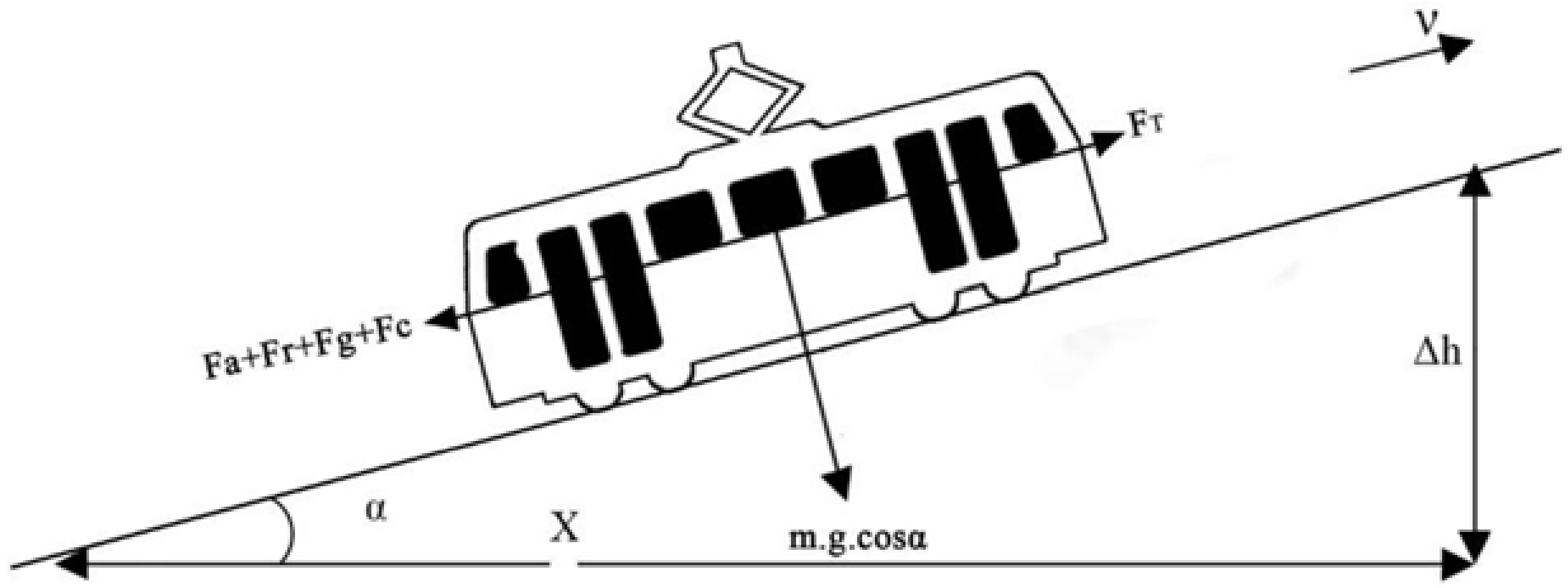
This paper uses the kinematic method. This method applies the train trajectory to calculate power at the wheel and, subsequently, input power at the catenary (and, ultimately, total energy consumption). Train trajectory includes acceleration (a), velocity (v), and traveled distance (x) diagrams over time. Based on Newton’s second law, traction motors must accelerate the vehicle and overcome the driving resistances:
where F
T is the tractive force in (N); m is the vehicle mass plus loading, and R(total) is total driving resistances against the movement direction.
Figure 1 depicts a schematic representation of applied forces to the rolling stock.
Driving resistances include the two most important kinds—aerodynamic resistance and rolling resistance, and two extra resistances related to the infrastructure conditions—gradient resistance and curve resistance. Passenger service must certainly consider overcoming auxiliary systems, such as the heating, ventilation, and air conditioning (HVAC) system, which is essential in passenger comfort issues.
In the railway system, the Davis formula [
16] was used, for a long time, as a reliable equation to calculate the total resistance. However, The American Railway Engineering Association (AREA) has improved Davis’s original formula to better reflect onto the rolling [
17]. The resulting formula is valid for most kinds of trains:
where R(total) is the total rolling resistance in pounds-force, w is the weight per axle in tons, n is the number of axles, b is the friction coefficient, V is the velocity in miles per hour, K is a lumped coefficient for aerodynamic resistance, and G is the grade in percentage (positive for uphill slopes and negative for downhill slopes).
The motion diagram by a tram between two stops may be divided into three different phases: acceleration, constant speed, and braking. The largest energy consumption takes place during the acceleration phase [
18]. To calculate the instantaneous acceleration amount, the experimental method onboard the tram by a GPS mobile application’s so-called Phyphox was examined. Phyphox was created at the second Institute of Physics of the RWTH Aachen University; it allows users to use sensors in their smartphones for their experiments. For example, to detect the acceleration-time graph using an accelerometer [
19]. Final energy consumption can be calculated by integrating the instantaneous force over the traveled distance [
20]:
Alternatively, the required power, P
e can be calculated as:
3. Case Study of Pankow District of Berlin, Germany
Dating back to June 2018, five important parcel delivery companies in Germany have participated in a one-year pilot micro-depot process in Berlin. Hermes, DHL, DPD, UPS, and GLS unloaded all truckloads in a joint depot in the Mauerpark area. Cargo bikes picked up the cargo, used the containers as a secure base, and delivered the individual packages to the 800,000 residents who lived within a 3 km radius [
21].
In regards to the press release of the KoMoDo project results, dated 22 May 2019 [
22], during the one-year project period, extensive findings were gathered. The use of cargo bikes on the last mile was environmentally friendly, and journeys with conventional delivery vehicles were replaced. The delivery staff mainly used electrically-supported cargo bikes within a radius of up to three kilometers around the micro depot location in Prenzlauer Berg. As a result, they were emission-free, local, and able to save around 11 tons of CO
2 compared to conventional delivery vehicles. Up to 11 cargo bikes were in use every day, resulting in a total of over 38,000 km of driving and approximately 160,000 parcels delivered by Germany’s five largest parcel service providers over a period of 12 months (the project duration). Additionally, the providers involved were able to increase the parcel volumes delivered during the project.
Assuming that there were 2 days off in a week, with 261 workdays in the year—on average, they should have delivered 613 parcels per day (160,000/261 = 613 parcels per day). Considering that every 15 parcels fit in a 1 m
3 box, the daily cargo demand for the micro depot would approximately be equal to 41 m
3. Maximum volumetric calculation factors of the delivery companies in Germany belong to GLS, which is 250 kg/m
3 [
23], and the minimum to DHL, which is 200 kg/m
3 [
24]. By considering the maximum amount, micro depots might demand 10.25 tons per day.
3.1. Technical Characteristics of the Vehicles
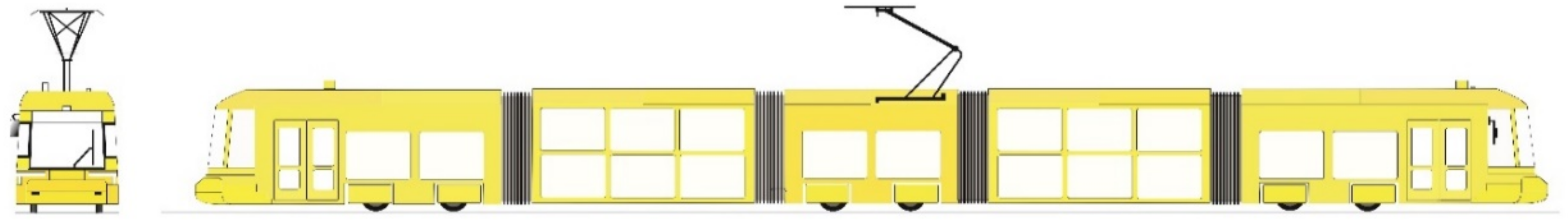
To execute the project, two types of tram vehicles were suggested by railway undertaking (RU). The first one was named Tatra KT4D, which is no longer in operation in Berlin tramlines; the second one, the most diffused vehicle in Berlin, was a Bombardier Flexity. Both vehicles required a redesign of the interiors, via a series of modifications, to achieve the proper conditions for cargo usage.
Table 1 shows the technical characteristics of the KT4D and Flexity Berlin.
Modified KT4D tram (
Figure 2) has a capacity of 12 shipping boxes or 12 cubic meters. To guarantee supply of the current and future demand of the KoMoDo depot, the vehicle can be coupled by two cargo coaches. As seen in
Figure 2, two coaches have space, respectively, for 28 and 24 m
3 of parcel shipment. Therefore, the total capacity of the combined KT4D tram would be 64 m
3, while the maximum allowed weight (wagon and load) of each coach is 30 tons.
According to
Figure 3, modified Flexity can carry out up to 36 shipping boxes, 2 transversally and 18 longitudinally.
3.2. Identifying the Tram Paths and Turning Loops as Loading Stations
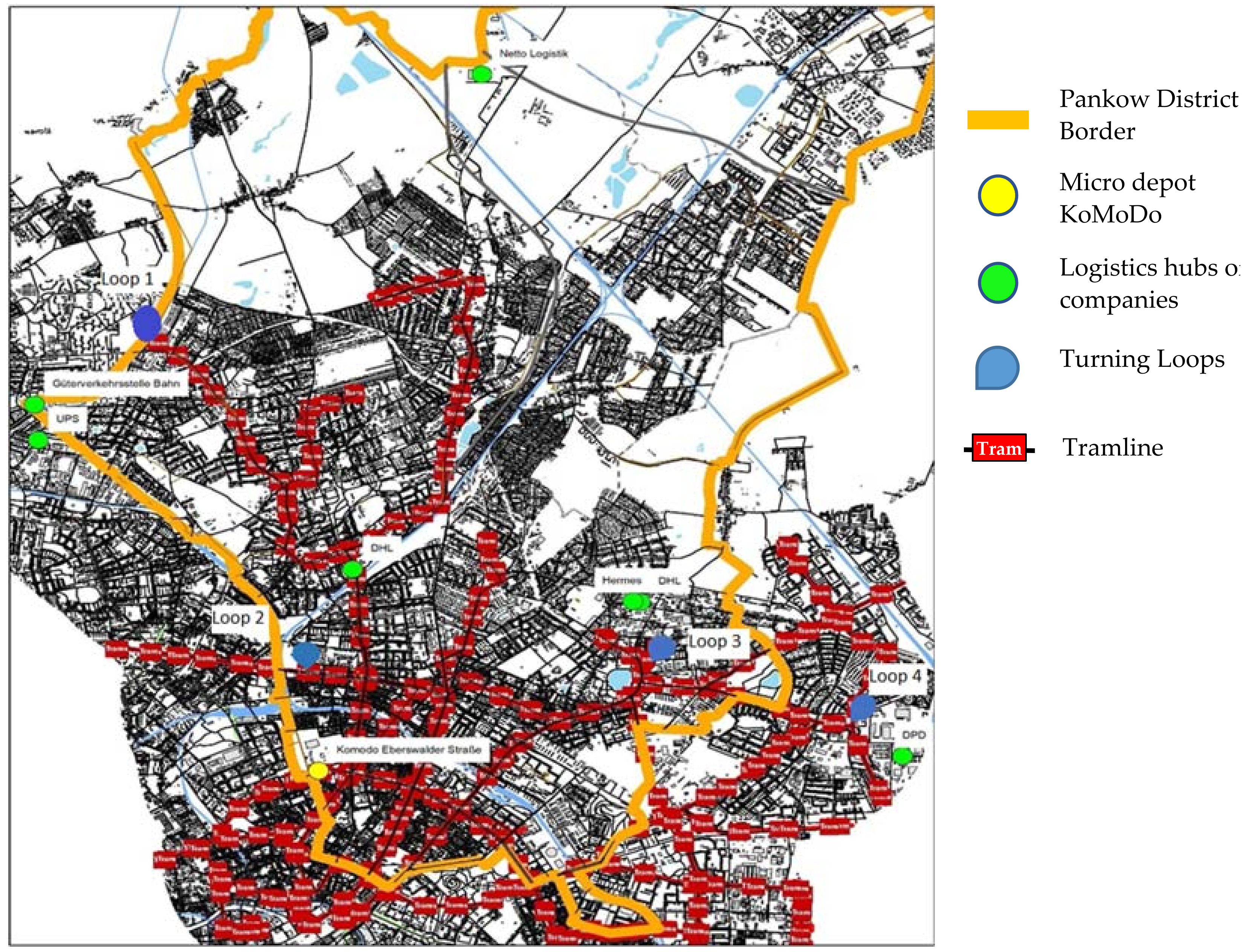
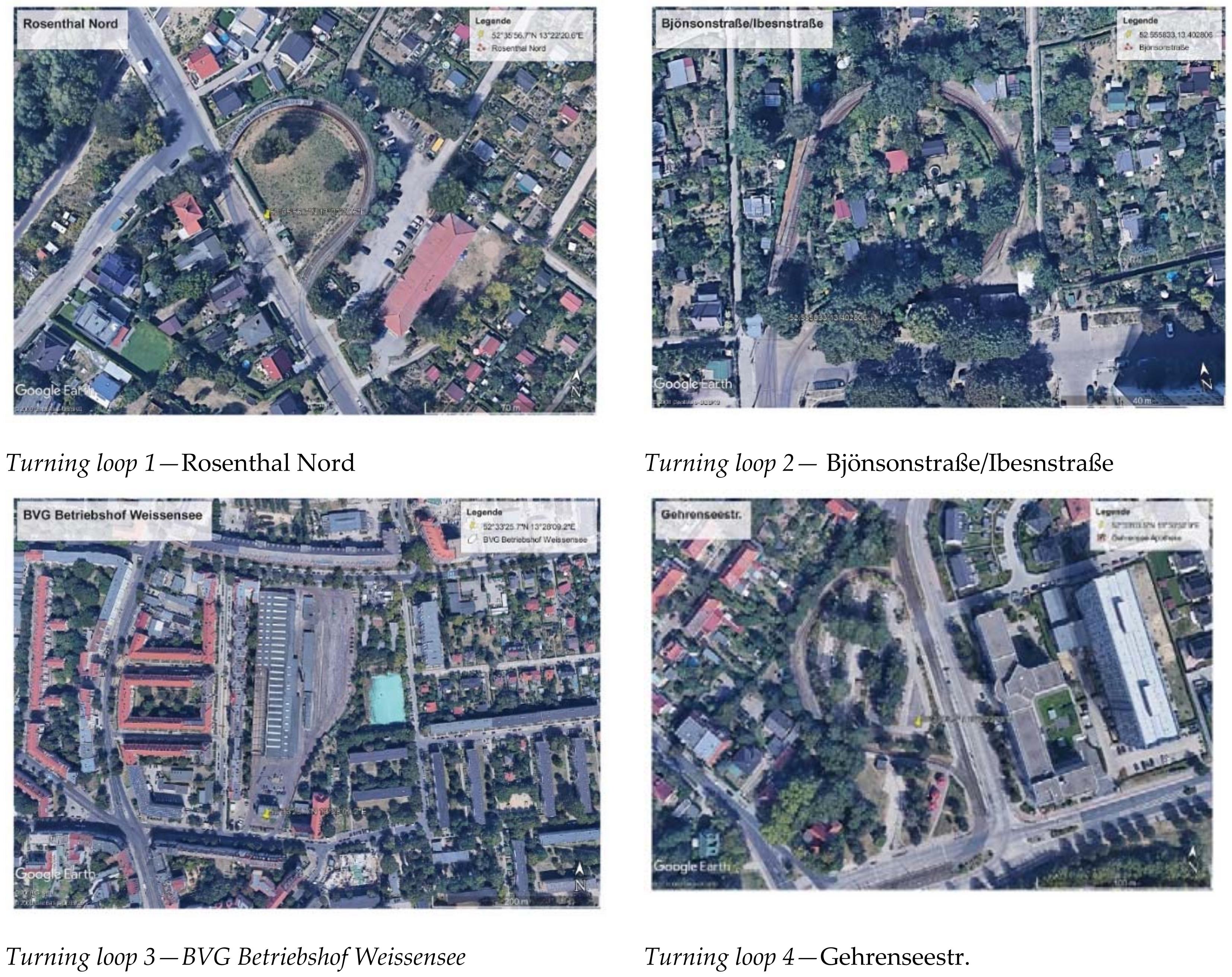
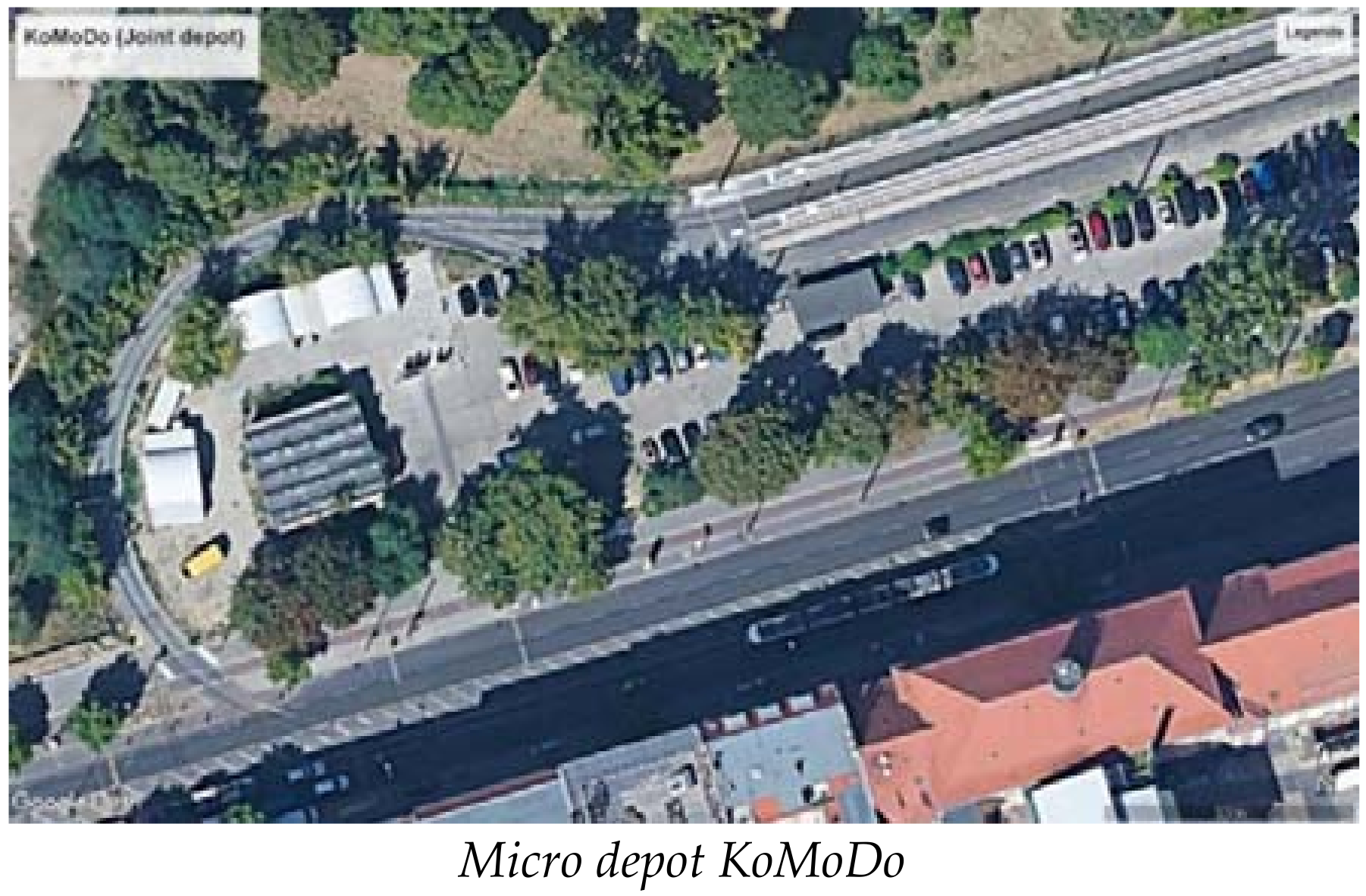
Figure 4 shows a map of the district of Pankow where the logistics hubs of parcel delivery companies are marked by green points. The yellow circle in the Eberswalder Straße is the micro-depo ‘KoMoDo’, where five logistics companies transport their parcels on the last mile by cargo bike. The blue circles present the existing turning loops on tramlines. The turning loops would be the most appropriate stations to load the company goods onto the freight tram to avoid interrupting the passenger service. As a result of the in-site investigation, loops 3 and 4, possessing the sidings to the track, will have no difficulties interfering with passenger tram departures. Loops 1 and 2, on the other hand, have just one track—but regarding a 10 min headway of tramline 50, at turning loop 2, and 15 min of line M1 at turning loop 1, will be enough time for a tram to be loaded.
The selected routes should use the existing infrastructure of lines along cargo hubs to deliver to the micro depot by tram and not by a lorry as hitherto. The tramlines involved in routes that would partly share their paths with the freight trams are M1, 50, M13, M2, 12, M4, 27, M5, M17, and M10.
Loading stations (turning loops) which have been shown in
Figure 5, should be covered by the chosen paths. The path operating by a single-vehicle must cover all four loops, or by two vehicles, where each must cover two loops.
Due to parcel delivery conditions, fewer interruptions with passenger services, and less delay—transport and goods handling should be performed in the daytime, at a non-peak time. Considering tramline headways, there are different sections of railways (i.e., in terms of rail occupancy). For instance, the section from Rosenthal Nord to Pastor-Niemöller-PL offers 15 min headway at which the freight tram can run with no braking at the stops, while the freight tram on the section from Antonplatz to Berlliner allee interfaces with three lines, with a maximum headway of 3 min between two sequence trams. However, measuring the exact arrival time and the delay of the freight tram would require a simulation model, which is not the concern of this study.
3.3. Possible Scenarios
Scenario 1: the first scenario considered a single vehicle for the micro depot delivery, which would combine the Tatra KT4D by the cargo coaches, due to its major capacity (up to 64 boxes). The journey begins from loop 1, where the vehicle will be loaded with company goods, and runs into loop 2; after being loaded at the second loop, according to
Figure 6, it moves to loops 3 and 4 instead, to directly reach the micro depot. After stopping and being loaded at four loading stations (red lines), it travels to the KoMoDo micro depot through the shortest path (green lines). The traveled distance by the freight tram in this scenario is 26.78 km.
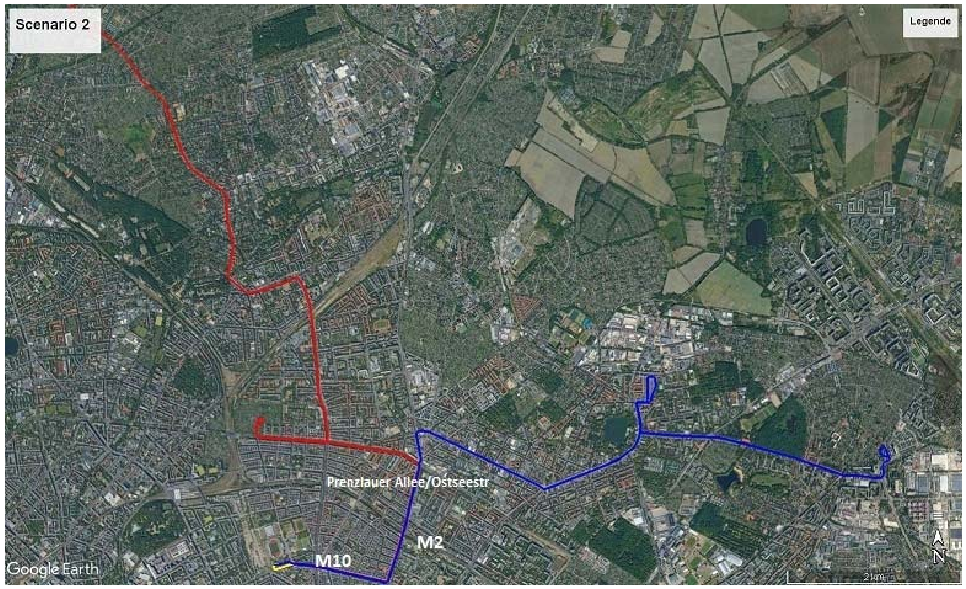
Scenario 2: in this scenario and the next one, the analyses were performed based on delivery by two vehicles (KD4T and Flexity). In the second scenario, according to
Figure 7, the Flexity tram journey begins from loop 1 and travels through the red path, whereas the KD4T tram journey starts from loop 4 and continues the blue path. Both vehicles, to deliver to the micro depot, share the same track from the Prenzlauer Allee/Ostseestr stop, which may be used by both M2 and M10 lines. The traveled distance by the Flexity tram is 12.30 km and by the KD4T tram is 10.58 km.
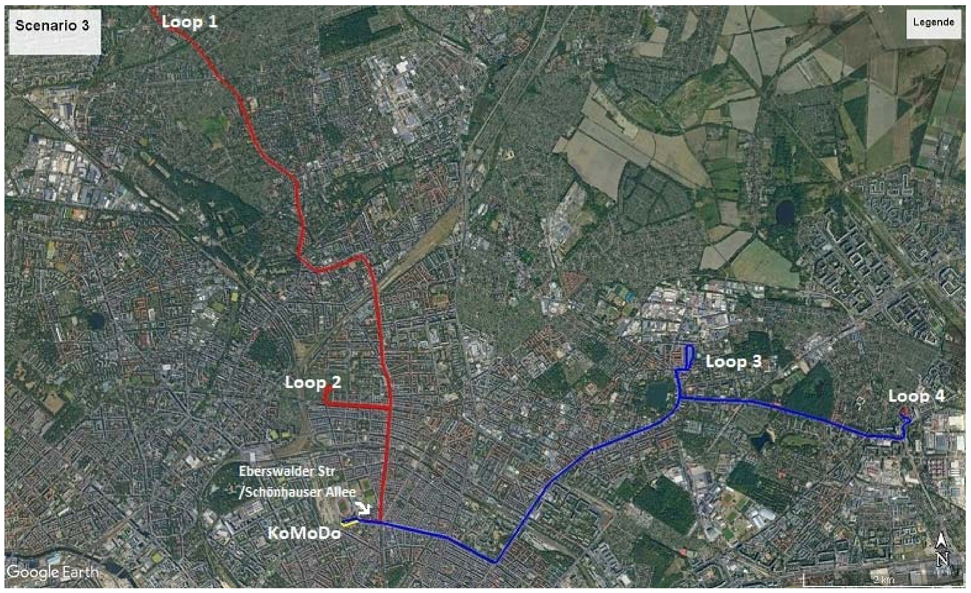
Scenario 3: As can see in
Figure 8, this scenario has the same condition as scenario 2. However, the difference is that the trams do not share any path, except a little section from the Eberswalder Str/Schönhauser Allee intersection to the micro depot. The traveled distance by the Flexity tram is 10.76 km and by the KD4T tram is 10.17 km.
Routing of a tramline is usually based on the shortest path, the lowest delay, the least occupancy of the infrastructure, and the coverage of areas most in demand for transportation. Since the purpose of this tramline execution is freight transport, these factors fall into the next priority level. According to the current daily cargo demand of the micro depot, the freight tram can provide it all just by one run per day. The tram does not need to stop at every station along the route, except four turning loops for loading company goods. Nevertheless, the comparison of the alternatives would be carried out, based on less energy consumption and more energy efficiency, which has a significant environmental and economic impact.
3.4. Acceleration, Speed, and Distance Plot
As previously mentioned, the acceleration amount was measured by an experimental method onboard the tram using the Phyphox mobile application.
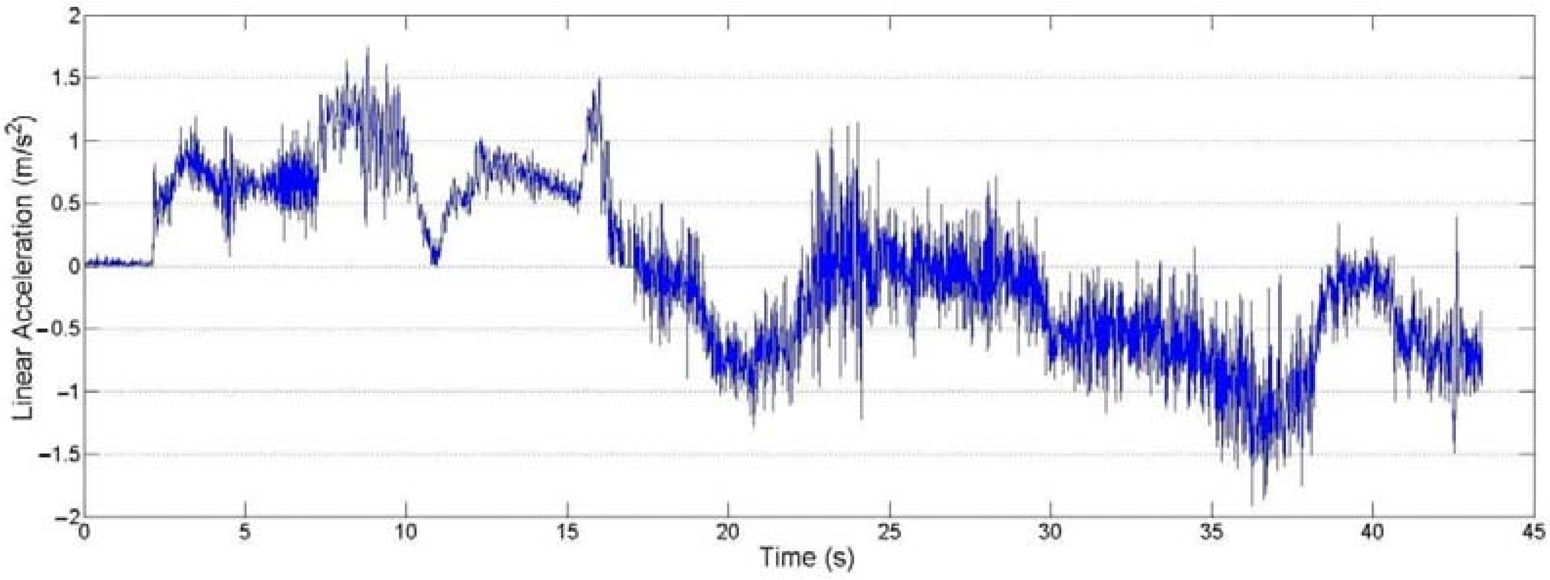
Figure 9 is a sample of Phyphox results that demonstrates the instant accelerations of a Flexity passenger tram of line M1, between two stops, for 43 s. As can be concluded, there is no constant acceleration in real cases. However, for simplifying the comparison process and consumption measurement, a constant acceleration value during each motion phase, as close as possible to reality, was assumed. According to
Figure 9, the average acceleration for a Flexity tram is 0.75 m/s
2, and the average deceleration is −1.2 m/s
2. Due to not considering passenger comfort in a freight tram case, acceleration can be increased up to 1 m/s
2.
Therefore, we can theoretically drown the velocity-time graph (
Figure 10) for our freight tram path. In the acceleration phase, the vehicle runs from a standstill to the speed of 36 km/h with an acceleration value of 1 m/s
2, and then changes acceleration gradually to zero; it continues with constant speed. To stop the vehicle at an intersection or a station, it brakes with deceleration −1.2 m/s
2.
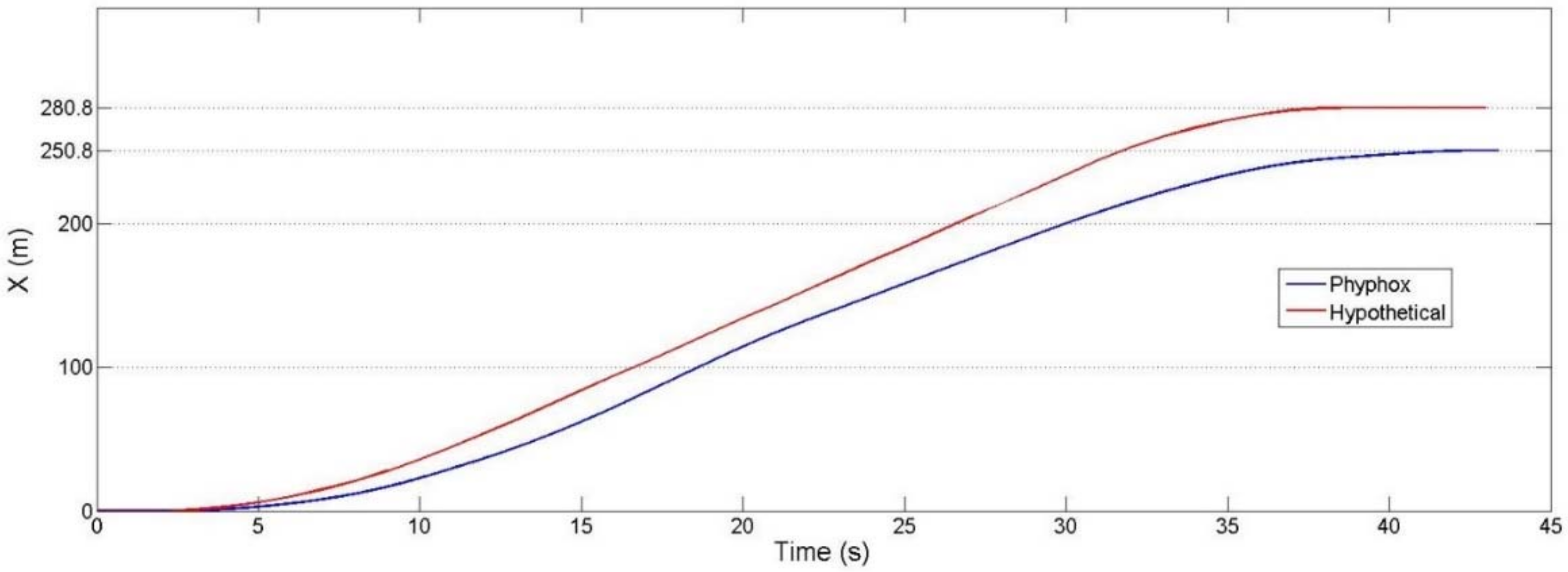
Figure 11 shows the hypothetical and real distance-time graph of a Flexity tram, resulting from the speed-time graph of
Figure 10. As can be seen, the tram vehicle traveled 280.8 m based on the constant acceleration assumption. On the other hand, it traveled 250.8 m based on instantaneous accelerations measured by the Phyphox application.
To examine the vicinity of our results from a hypothetical vehicle function, and real one, we obtained the energy consumption in both cases, using
Figure 10 and
Figure 11 as speed and distance plots, and
Figure 12 as a tractive force diagram. The drawn tractive force diagrams resulting from instantaneous velocities and accelerations are explained in the next section.
3.5. Calculating Tractive Force and Energy Need
The ability to calculate gradient and curve resistance demands very detailed knowledge of the tracks. Since this knowledge is rarely available, and is negligible in mainly flat lands, such as in Berlin, these kinds of resistances are not considered in the consumption measurement.
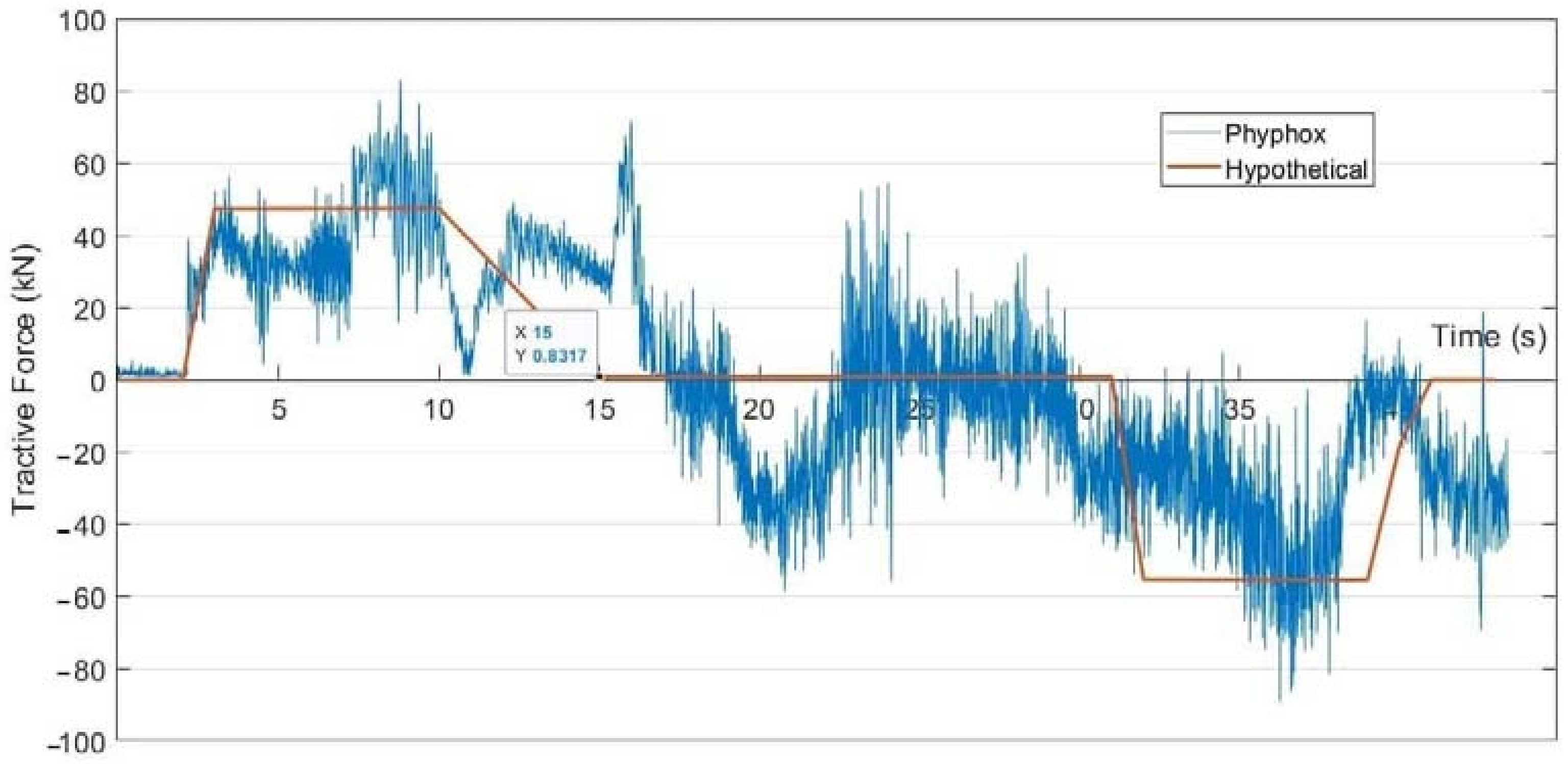
Assuming vehicles running on flat tracks with a friction coefficient = 0.01 and lumped coefficient = 0.3, the tractive force diagram of a Flexity tram on the same section of graphs 9 and 10 will be
Figure 12. Additionally, it should be noted that the weight of the vehicle has been supposed with max load capacity, which is 46.9 tons; 36 boxes × 250 kg + 38,900 kg. Due to the comfort function in freight service not mattering, auxiliary system efforts, which usually take 20% of the total needed energy, was not considered.
To draw the Pe graph of the mentioned sections, having tractive force trends (
Figure 12) would be enough to multiply the instant velocity in the corresponding force. Afterwards, to estimate energy consumption, the instantaneous force should be integrated over time. Since the tram is not equipped with an energy storage system to collect dissipated energy during braking, the integration should be applied on just the positive part of the power trend, exactly before the vehicle starts to brake and acceleration becomes negative.
As a result, the needed energy for a Flexity freight tram traveling 280.8 m, with a hypothetical speed profile, and 250.8 m, with real speed profile, in regards to the described assumptions above, can be obtained as the following integration:
The calculation demonstrates that, if the tram travels between two stops with a hypothetical speed profile, it would save 14% energy consumption. Nevertheless, the needed energy of the vehicle for each scenario is measured by assuming constant acceleration, constant speed, and constant deceleration along each section.
3.6. Quantity of Braking and Acceleration along the Freight Tram Route
The most important issue for calculating the energy consumption of trams in different scenarios is looking at how many times the freight tram should brake, until it stops and re-accelerates to the maximum speed during its journey to the KoMoDo micro depot.
For this purpose, we divided the tram route of each scenario into sections, where the freight tram with high probability has to stop and reaccelerate. The braking spots, defining the end points of the sections, were selected based on traffic restrictions, such as traffic lights, intersections, and tram stops with high passenger service frequency. For instance, the 26.54 km route of scenario 1 operated by a single vehicle was divided into 63 sections. This implies calculating total consumption of the KT4D on scenario 1, based on supposed assumptions, drawing 63 tractive force graphs over time, calculating needed energy for each section.
Some of these sections have very short distances, where the vehicle does not have enough time to reach the maximum speed (50 km/h) measured by the mobile app in the Pankow district.
Table 2 indicates the speed limits of various sections in respect to their distances.
3.7. Confronting Scenarios Based on Energy Consumption
3.7.1. Scenario 1
Due to the major capacity of the combined KT4D tram, this scenario is carried out with a single KT4D tram. The KT4D speed-time pattern obeys the same pattern of Flexity. Total consumed energy is obtained by the sum of energy needed for each section during the whole route. Two amounts are dependent upon the weight of the vehicle. The first one is the maximum load, which means 22.54 tons of tram besides 2 × 30 tons (max tolerated load by axels) of cargo coaches, making 82.54 tons in total. For another one, regarding the current daily demand of the micro depot, the tram could be coupled with just one cargo wagon to supply it, with a total weight of the vehicle equaling 52.54 tones.
Table 3 and
Table 4 demonstrate the divided sections along the scenarios, beside the corresponding traveled distance and time and energy consumption.
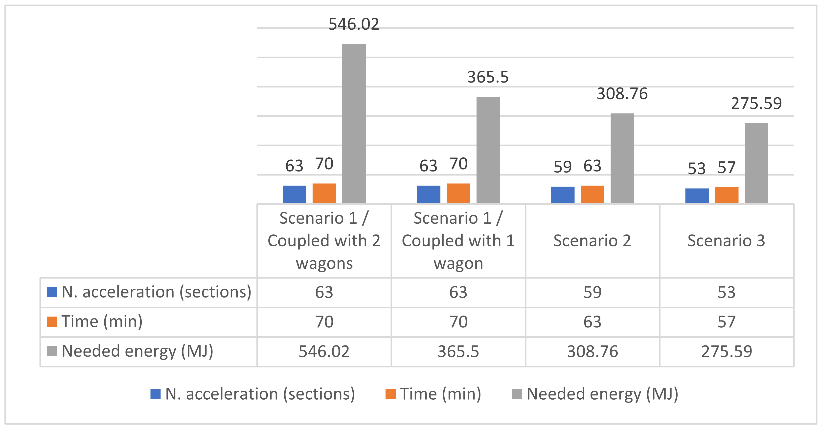
As the results show, a Tatra KT4D with two cargo coaches needs 546.02 MJ energy and 70 min to operate the defined route of scenario 1, in an ideal condition. The ideal condition intends that the tram, in different sections, can continue at a constant speed without acceleration until it should brake to stop. The traveled time has been calculated by summarizing section time duration plus 20 s of idling time. A KT4D with a single cargo coach, in turn, needs 365.5 MJ.
3.7.2. Scenario 2
Scenario 2 must be operated by two vehicles, on two separate routes. The longer route (turning loop1 and 2) is run by Flexity tram due to its lower weight and another one by KT4D. Both vehicles have sufficient capacity to cover half of KoMoDo’s demand. Due to the continuous increase of urban freight demand, we suggest considering the maximum load for each vehicle.
Table 5 and
Table 6 show results of freight delivering to the micro depot across the scenario 2 sections. As can be concluded, vehicles need a total of 308.76 MJ, 154.97 MJ for Flexity and 153.7 MJ for KT4D. Moreover, Flexity needs 34.5 min and KT4D 28.2 min to reach the KoMoDo micro depot.
3.7.3. Scenario 3
Scenario 3 has almost the same circumstances as scenario 2, except for their routes. As the results show in
Table 7 and
Table 8, Flexity tram consumes 128.44 MJ power and 29 min time, and KT4D consumes 147.15 MJ and approximately 28 min in. Therefore, this scenario requires a total of 275.59 MJ of energy.
3.8. Results
Finally,
Figure 13 presents a comparison based on energy consumption. The case study results show scenario 3 is the best route between three scenarios, where the freight tram system can reach the KoMoDo micro depot, having the lowest duration time and lowest consumption. Scenario 1, with KT4D in a single composition, could be responsible for current daily freight demand of the KoMoDo, while other scenarios were considered with a maximum loaded vehicle to supply future demand as well. One effective factor that impacts final energy consumption is traction system efficiency. The lower efficiency of the older Tatra KT4D tram makes the situation of scenario 1 not affordable due to high consumption.
4. Reduction of CO2 Emission
One liter of diesel weighs 835 g. Diesel contains 86.2% of carbon or 720 g of carbon per liter. In order to combust this carbon into CO
2, 1920 g of oxygen is needed [
26]. The sum is then 720 + 1920 = 2640 g of CO
2 /liter diesel. An average consumption of 5 L/100 km then corresponds to 5 L × 2640 g/L/100 (per km) = 132 g CO
2 /km. A common truck type to transport parcels in Berlin is Mercedes-Benz Atego, which consumes 17 l/100 km [
27], and as a result, emits 448 g/km CO
2.
Figure 13 illustrates the current travel distances from six company logistics hubs to micro depot KoMoDo. The distances traveled to the turning loops are specified in
Figure 14 by Google Maps as well. The freight tram system will eliminate the differences between current and future truck-kilometers. For instance, from the GLS hub to KoMoDo, and back, it would mean 10 km ((8.8 – 3.8) × 2) less of truck millage. Likewise,
Table 9 shows a truck-kilometer reduction from the logistics hubs in the case of freight tram operation. Consequently, a freight tram system can potentially reduce 60.4 km of road commercial vehicle traffic per day. Considering there are 261 working days in Berlin, CO
2 emission is expected to decrease by more than 7 tons.
5. Conclusions and Discussion
Nowadays, major European cities are facing huge challenges in regards to traffic congestion. Therefore, any solution that would lead to the reduction of trucks on the road should be taken into consideration. Using a tram vehicle, specially adjusted to freight transport to distribute goods along the network, is a possible solution.
The study took a systematic approach, based on identifying scenarios, traveled distances, and time durations, and appraised the scheme through an energy consumption analysis to assess a hypothetical freight tram scheme in Berlin. The study also deemed energy efficiency as an important aspect for routing a tramline, besides the shortest path, service demand, traffic congestion, and delay. At first, scenarios were identified based on other aspects, and then the needed energy measurement for each scenario was applied. Scenario 1 was identified based on the parcel delivery by a single KT4D tram coupled with one and two cargo coaches. The tram travels 26.78 km of the selected tram path by itself, and should stop and reaccelerate at 63 pre-defined sections. In scenarios 2 and 3, however, two separate trams (KT4D coupled by one cargo coach and Flexity) perform the shipment. KT4D travels 10.58 km, with 26 sections in scenario 2, and 10.17 km with 26 brake spots in scenario 3. Flexity, on the other hand, should complete the alternative route of scenario 2 by 12.3 km, including 33 sections, and the rout of scenario 3 by 10.76 km, including 27 sections. Finally, a comparison based on energy consumption was conducted. The results show that scenario 3 is the best route between three scenarios, in which the freight tram system can reach the KoMoDo micro depot with the lowest duration time and lowest consumption.
A typical example of an interoperable public transport system with a constrained guide is the so-called “tram-train”, which achieves integration between the tramway and the railway, using suitably modified tram vehicles, such as the trams of the German city of Karlsruhe, or specially designed, such as the Kassel RegioCitadis vehicles, to be able to travel on both types of infrastructure [
28]. As major parts of distribution centers are outside of metropolitan areas—a freight tram-train system can transport the goods directly to a joint depot and skip shipment by trucks. A future study will be a feasibility assessment of the freight tram-train system to deliver to a joint depot from a joint distribution center, especially for parcel delivery companies.


