Abstract
Although the Korean government plans to increase its share of variable renewable energies (VREs), the Korean power market is not sufficiently mature to accommodate a large increase in VRE generation. Thus, the Korean system operator plans to introduce a two-settlement, and an imbalance settlement is also under consideration, among several options. Therefore, this study analyzes how many incentives are given for prediction accuracy under several imbalance settlement schemes adopted from European and US power markets. Results show that the imbalance settlement consisting of threshold and penalty terms is useful for rule-makers, who can control revenue differences between the groups with different prediction accuracies by adjusting the two terms. The suggestion given in the paper will be useful for not only the Korean power market but also for the countries that plan to establish the imbalance settlement rules while increasing renewable energy.
1. Introduction
To reduce greenhouse gas emissions in response to global warming, power generation from variable renewable energies (VREs) is expanding worldwide [1]. At the United Nations Climate Change Convention held in Paris, France, on 12 December 2015, 195 parties signed the Paris Agreement that accelerated the energy paradigm shift to move to low-carbon energy systems. Accordingly, the Korean government has set a target to reduce CO2 emissions by 37% compared to the Business-as-Usual scenario by 2030 [2]. To achieve this target, the Korean government plans to increase the share of VREs, including photovoltaic (PV), wind turbine (WT), and hydropower sources, from 7% in 2016 to 20% in 2030. Among these sources, PVs and WTs are the most prominent components in increasing VRE generation.
VREs are characterized by high variability and uncertainty, because their outputs are affected by weather conditions such as solar radiation and wind speed. The uncertainty and volatility of VREs can threaten the reliability of a power system and increase operating costs [3,4]. Leading countries that have increased their VRE share production rates faster than Korea already have market rules capable of handling the volatility and uncertainty of the VREs [5,6,7,8]. One of the rules is an imbalance settlement [9]. The imbalance settlement lets market participants be responsible for their market bids and offers and settles the difference between the winning offer and actual output at an imbalance price.
The imbalance settlement can incentivize dispatchable generators and flexible loads to accurately follow dispatch signals from the system operator (SO). In addition, the imbalance settlement can incentivize non-dispatchable generators and non-flexible loads to present more accurate forecasts. However, the introduction of an imbalance settlement at the VRE promoting stage can act as an obstacle that slows the achievement of policy goals by deteriorating the profitability of the VREs. In leading countries, imbalance settlements were introduced during the deregulation process rather than in the VRE promotion stage. Therefore, temporary and partial exemptions have been applied as a reasonable compromise between the imbalance settlement and the VRE promotion [10].
On the other hand, under current Korean power market rules, the VREs do not submit forecasts and are not responsible for their imbalances. As the generation of the VREs without accurate forecasts increases, the uncertainty in the power system will also increase. According to the current market rules, the responsibility for the increasing uncertainty is entirely passed on to the SO [4]. In addition, the balancing cost incurred by the imbalances is finally passed on to a retail company and delivered to end consumers. Therefore, it is necessary to introduce a reasonable cost allocation through the introduction of the imbalance settlement and to ensure that each market participant has its financial responsibility for its imbalances.
Several studies have analyzed the impact of imbalance pricing on the VRE revenue [11,12,13,14,15]. Wan et al. studied the impact of the imbalance settlement rule of the United States on WTs [11]; Brunetto and Tina applied the imbalance pricing rule of Italy [12]; and Chaves-Ávila et al. compared the imbalance pricing rule of Belgium, Denmark, Germany, and the Netherlands [13]. In [11,12,13], since a single WT generator was subject to study, the generator was assumed as a price taker. However, as the number of VREs and the proportion of their generations increase, their output and their imbalance affect day-ahead and real-time market prices. Thus, to consider the impact of VREs’ generations on the prices, the VREs are assumed as price makers in this study, as in [14,15]. Haring et al. carried out the allocation of reserve costs via imbalance settlement benchmarking Nordic power markets and Switzerland [14]. In [15], Wu et al. compared one pricing, two pricing, and dual pricing schemes considering multiple criteria, including forecast accuracies and incentives to invest in flexible resources.
For the regulators who are trying to achieve the CO2 emission targets, it is important to make potential VRE investors invest in the VREs. On the other hand, for the potential VRE investors, expected revenues and risk of the revenues are important information for the investment decisions [16]. However, since [11,12,13,14,15] considers a single or a small number of VREs, only the revenues of a small number of VREs were analyzed, which is not sufficient to show the expected returns and risks. Therefore, we assumed more than 1000 VREs to figure out the expected returns and the risks. Furthermore, the VREs are considered the price maker. This study estimates the distribution of the VREs’ revenue including the expected values and the standard deviations of the revenues through market simulations. Furthermore, the VREs are also grouped by resource, prediction accuracy, and whether an imbalance of a VRE increases or decreases system imbalance. The revenues of the VRE groups are analyzed under several imbalance settlement schemes.
The Korean electricity market has not been sufficiently matured to accommodate the increased number of VREs as planned [2]. Thus, the Korean SO plans to introduce a real-time market, and an imbalance settlement is also under consideration, with several options referring to other leading power markets. The purpose of this study is to determine a suitable imbalance settlement for the Korean power market. More specifically, this study quantitatively analyzes how much incentive for prediction accuracy is provided under each imbalance settlement rule. The results of this study will be useful for the countries that plan to establish the imbalance settlement rules while increasing renewable energy.
The remainder of this paper is organized as follows: Section 2 describes the background of the study, including the Korean power market. The formulation of each imbalance pricing is presented in Section 3. In Section 4, the settings of case studies are described. In Section 5, the revenues of the VREs are compared according to the forecast accuracy under various imbalance pricing cases. The results are discussed in Section 6, and the conclusions of the study are provided in Section 7.
2. Background
2.1. Settlement of Variable Renewable Energy in the Korean Power Market
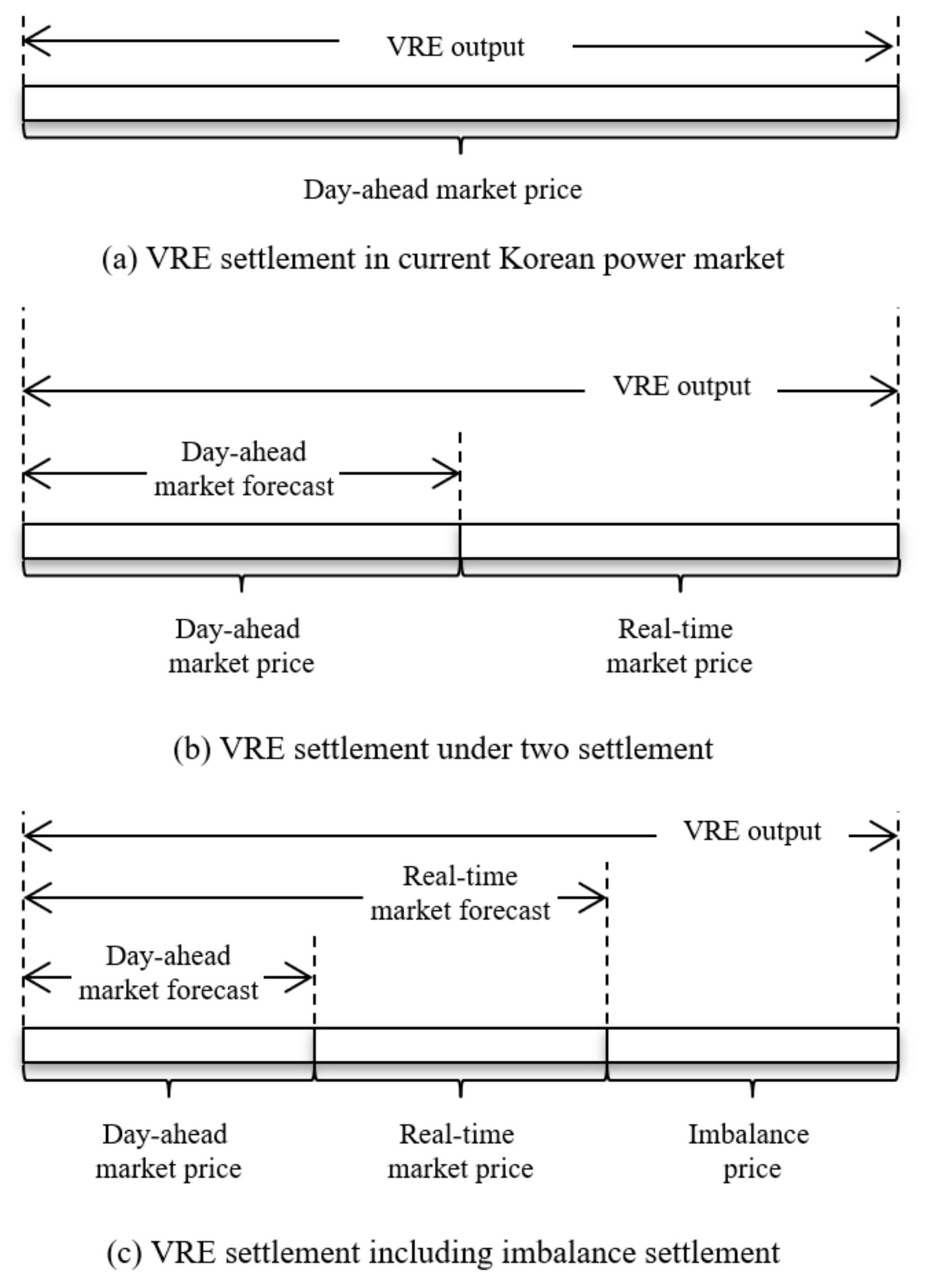
The Korean system operation model comprises a centralized dispatching model [17]. The Korean Power Exchange (KPX), an independent SO (ISO), operates a day-ahead market (DAM) and Korean power system in real-time [18]. Because the ISO does not operate a real-time market (RTM), the RTM price is not calculated. Thus, the VREs receive payment of their generation at the DAM price, as shown in Figure 1a [19]. In this settlement rule, the ISO cannot incentivize the VREs to make more accurate predictions on their generation. Without the incentives, the increase in VREs will increase the uncertainties in the power system, which makes it difficult for the ISO to operate its system reliably. Furthermore, the balancing cost incurred from the imbalances of the VREs is finally passed on to the sales company and delivered to the end consumers.
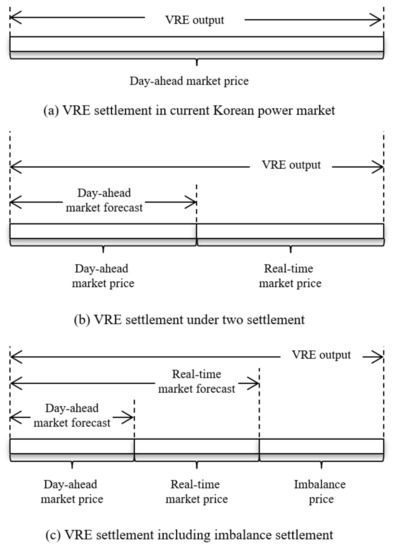
Figure 1.
Settlement of variable renewable energy (VRE) (a) under current Korean power market rules, (b) under a two-settlement, (c) and including an imbalance settlement.
2.2. Real-Time Market and Imbalance Settlement
As one of the solutions to the problem in the Korean power market, the ISO announced a plan to introduce real-time pricing in the Korean power market that would enable a two-settlement approach. As shown in Figure 1b, the two-settlement pays the generation of the VRE using the DAM price and the RTM price. As a VRE submits the output forecast to the DAM, then the accepted bid is settled at the DAM price. As the time becomes closer to real-time, the VRE submits an updated forecast into the RTM, and the accepted bid is settled at the RTM price. Thereafter, the difference between the final output and the DAM forecast is settled at the RTM price. This two-settlement is widely used in the North American power markets [20].
The VRE forecasts submitted to the RTM can differ from the actual output, as it is submitted several hours before the actual delivery time. The difference between the two is called an imbalance, and the imbalance is settled at the RTM price in the two-settlement approach [21]. The imbalance can be settled at the so-called imbalance price, as shown in Figure 1c. By adding a penalty term to the imbalance price, ISO can induce market participants to reduce their imbalance. The rules for designing the imbalance price vary depending on the power market.
In this regard, it is necessary to figure out whether the two-settlement can give VREs the incentive to accurately predict their outputs. Therefore, in this study, we investigate whether the two-settlement approach provides any revenue difference to the groups with different prediction accuracies. Furthermore, results from other imbalance pricing methods that benchmark several power markets are also compared.
3. Settlement for Variable Renewable Energy
3.1. Composition of Settlement
The energy settlement to a VRE consists of the sum of the DAM settlement, the RTM settlement, and the imbalance settlement, as shown in Equations (1) and (2):
where is the annual sum of the total settlement of generator g; is the total settlement of generator g at time t of day d; and , , and are the DAM settlement, the RTM settlement, and the imbalance settlement of generator g at time t of day d, respectively. D is a set of days in a year, and T is a set of settlement periods per day.
The DAM settlement and the RTM settlement are calculated as follows (Equations (3) and (4)):
where and are a DAM price and an RTM price at time t of day d, respectively; and are the cleared generation in DAM and RTM of generator g at time t of day d, respectively.
3.2. Imbalance Settlement
The imbalance settlement method varies from SO to SO. Five imbalance settlement methods used in the actual market are compared. Originally, some of the presented pricing methods are applied only to traditional centralized power generators; however, those methods are also selected to compare the impact on the VREs’ revenue.
3.2.1. Type I: Real-Time Pricing—The United Kingdom and PJM
The commonly used method for pricing the imbalance is using the RTM price. The RTM price is one of the most cost-causing methods, because it reflects the marginal price of real-time balancing resources. In the UK, the marginal price of the balancing resource in the Balancing Mechanism is determined as the price of imbalance [22]. Similarly, in PJM, the real-time market price is used as the imbalance price [23], which is expressed by the following Equations (5)–(7):
where
where is the imbalance settlement under Type I; is an imbalance price; is a power imbalance; and is a metered output of generator g. Equation (5) is an equation for imbalance settlement, Equation (6) denotes RTM price is used for imbalance price, and imbalance is the difference between metered power and final position that is determined in RTM (Equation (7)).
3.2.2. Type II: Dual Imbalance Pricing—Fingrid of Nord Pool
In the Type I method, those who decrease the total system imbalance tend to earn higher returns in the total settlement, whereas those who reduce the system imbalance tend to earn lower returns. Thus, market participants can attempt to obtain higher profits by reducing total system imbalance. However, because this behavior increases the uncertainty factor from the perspective of the SO, Nordic SOs use dual imbalance pricing to suppress the generator’s arbitrary output variation [24]. In the progress of European market harmonization, Nordic TSOs planned to change the imbalance pricing from dual pricing to single pricing from the end of 2021.
Under dual imbalance pricing, as the generator’s imbalance increases the system imbalance, the imbalance is settled using the RTM price. However, as the generator’s imbalance reduces the system imbalance, the imbalance is settled using the DAM price, which is the penalty price for the generator. Therefore, dual pricing is operated to mitigate the risk of operational security caused by power oscillations in the system balance [25]. The equations of the settlement equation are as follows (Equations (8)–(11)):
where
else
where is the imbalance settlement in pricing Type II, and is the imbalance of the system, which is the sum of all participants’ imbalances.
3.2.3. Type III: Penalty on the Excesses—FERC OATT
In 1996, Federal Energy Regulatory Commission (FERC) presented FERC Order 888, including pro forma Open Access Transmission Tariff (OATT) for Promoting Wholesale Competition Through Open Access Non-Discriminatory Transmission Services by Public Utilities [26].
In FERC Order 888, one rule stated that the imbalance should be within ±1.5% or 1 MW. However, there were no imbalance settlement rules. Since then, in 2007, FERC Order 890 was revised to impose a penalty charge for excessive imbalances [27]. The rule is formulated as shown in Equations (12)–(17). In this regard, as a detailed formula is not provided, we have assumed that the penalty is applied only when the system imbalance worsens.
where
else
else
where is the imbalance settlement in pricing Type III, is the threshold of the power imbalance, is the threshold ratio of the power imbalance, and is the penalty ratio. The imbalance of the generator is exempted from the penalty price when the absolute value of the imbalance is smaller than the exemption threshold or (Equation (14)). When the absolute value of imbalance exceeds the threshold and the imbalance increases system imbalance, the price with penalty is applied (Equations (15) and (16)). In other cases, the RTM price is applied (Equation (17)).
3.2.4. Type IV: Do Not Pay the Oversupply—NYISO
In New York ISO (NYISO), imbalances of demand-side participants are settled on RTM price. However, stricter rules are applied to the generators. The generations exceeding the threshold are not paid [28]. The threshold applied to conventional generators is 3% of the capacity of each generator. On the other hand, the threshold applied to the WTs is 3300 MW that can be regarded as no penalty. This penalty is aimed at traditional generators, because they can arbitrarily adjust their output. Although the current rule to the WTs is meaningless, we modified the threshold value to compare this rule with other rules from other markets. However, the impact of the rule is also compared in consideration of the future when the relevant regulations are practically extended to the VREs. The rule is formulated as follows (Equations (18)–(20)):
where
3.2.5. Type V: Day-Ahead Pay on the Oversupply—MISO
In Midcontinent ISO (MISO), there are also rules aimed at traditional generators [29,30]. For an imbalance that does not exceed the threshold, the RTM price is used, and for the imbalance that exceeds the threshold, the imbalance is settled at variable cost. These can be formulated as follows (Equations (21)–(25)):
where
where is the imbalance price for non-excessive energy, is a non-excessive imbalance, is the imbalance price for excessive energy, is an excessive imbalance, and is the variable cost of generator g. Because VRE does not have a variable cost, the DAM price is alternatively used.
4. Simulation Settings
4.1. Categorization of Variable Renewable Sources
To compare the revenue changes of individual VRE, multiple VREs and their groups are defined. The size of each VRE is assumed to be 20 MW, which is the minimum size that can participate in the Korean power market. To meet the capacity of the large project VRE planned in 2030, we assumed that the total number of market-participating PVs is 726, of which the total capacity is 14.52 GW, and the total number of market-participating WTs is 460, of which the total capacity is 13.08 GW. To model some VREs that do not participate in the market, one equivalent generator of 19.01 GW of PV and 4.594 GW of WT is assumed.
We have also assumed that each VRE predicts the output and submits the prediction to the DAM and RTM. Four VRE groups are defined depending on whether the system imbalance increases or decreases and whether the degree of forecast error is large or small, as shown in Table 1.

Table 1.
Group of VREs participating in the wholesale market.
In the first letter, PV stands for the PV group, and WT stands for the WT group. In the second letter, B represents a group with large imbalances caused by inaccurate forecasting, and G represents a group with small imbalances resulting from accurate forecasting. Finally, in the third letter, the positive sign refers to aggravating groups that increase the system imbalance, and the negative sign refers to non-aggravating groups that reduce the system imbalance.
We have assumed that VREs are the only source of uncertainty in the market. Therefore, the sum of the imbalance of all VREs is equal to the system imbalance. To ensure that the direction of the system imbalance and the direction of the aggravating groups are the same, the number of VREs in the positive sign groups and the number of VREs in the negative sign groups are set to 2:1. In addition, we assume that non-market participating VREs cause imbalances in the same direction as the aggravating groups.
To focus on and compare the impact of the forecast error on the revenue of each VRE, we assume that the real-time outputs of all PVs are the same for all imbalance settlement strategies, and the real-time outputs of all WTs are the same for all imbalance settlement strategies. For each VRE, DAM and RTM forecasts are created by multiplying the VRE output and Gaussian noise. The DAM and RTM forecasts , are calculated as follows (Equations (26) and (27)):
For each of the groups with inaccurate forecasting (PVBs, WTBs) and groups with accurate forecasting (PVGs, WTGs), the error terms of the DAM and RTM follow a Gaussian distribution with averages and standard deviations, as listed in Table 2.
Table 2.
Gaussian distribution of each group’s forecast error.
For aggravating groups, the value of value is set to +1 on odd days and −1 on even days. On the other hand, for non-aggravating groups, the value of value is set to −1 on odd days and +1 on even days.
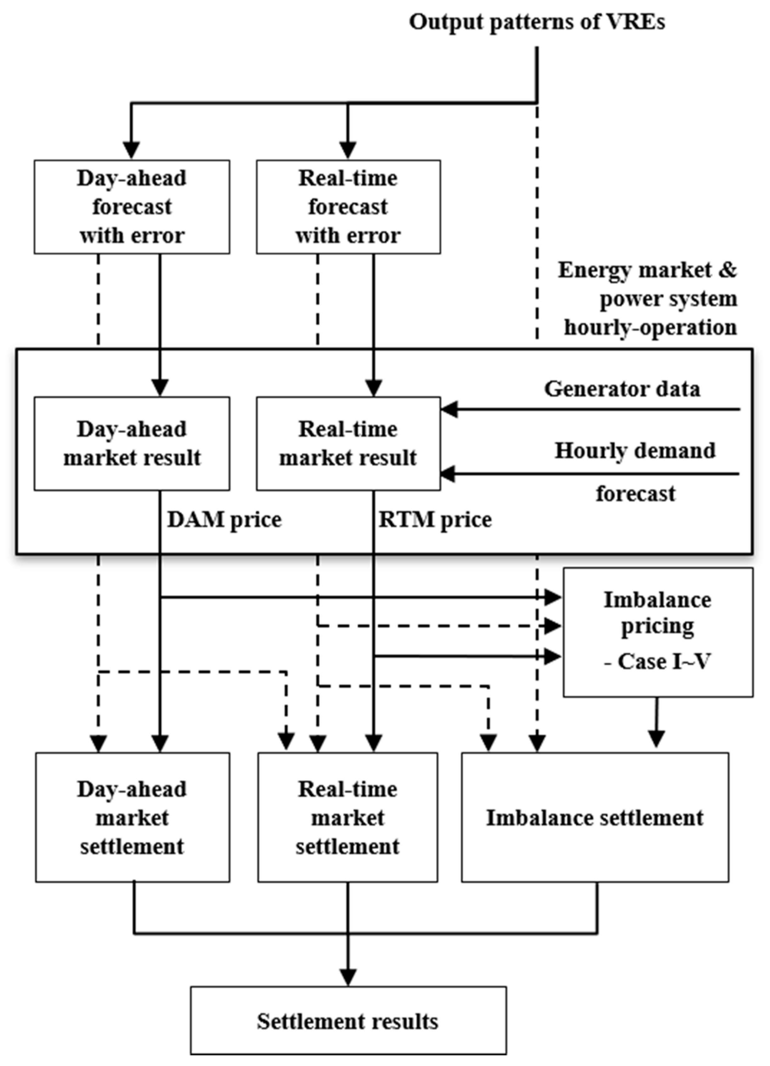
As shown in Figure 2, the simulations are performed to examine the revenue change of VREs caused by the size of the forecast error and various imbalance pricing. The power market is simulated using DAM forecasts, RTM forecasts, and the output of the VREs referring 2030 Korean market. The DAM price and RTM prices are calculated through a market simulation, and these prices are used to calculate the settlement for each VRE.

Figure 2.
Schematic diagram of the comparison of imbalance pricing schemes.
4.2. Market Simulation Settings and Results
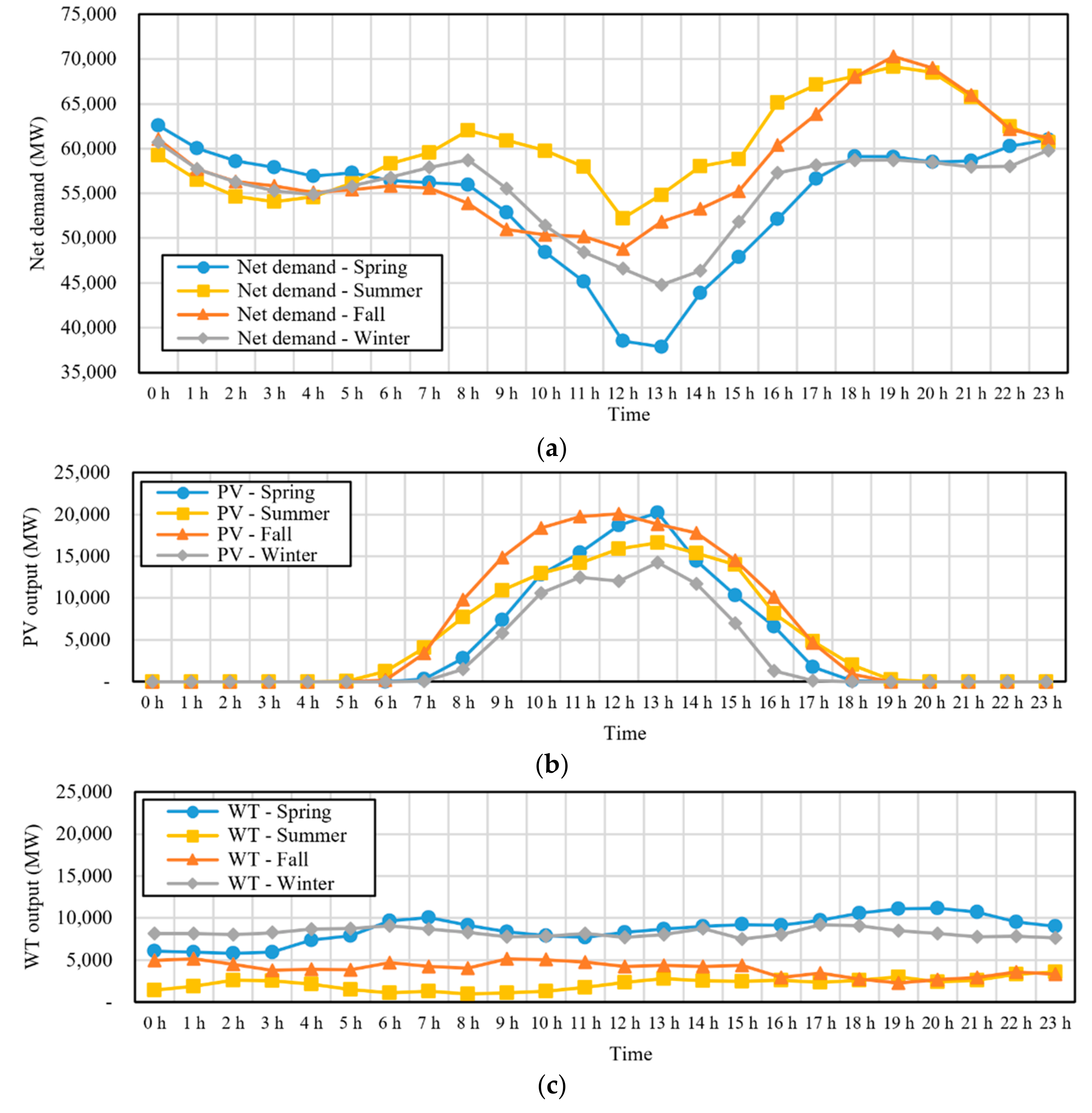
The patterns of the seasonal net demand, PV output, and WT output used in this simulation are shown in Figure 3. A demand pattern is derived by scaling up the demand pattern of 2019 to fit the gross demand in 2030 predicted in the 8th Basic Electricity Supply and Demand Plan [31]. The peak times of the net demand vary by season, but the valleys appear around noon in all seasons. Figure 3b,c show that PV output is the major factor that creates the valleys in the net demand pattern.

Figure 3.
Power patterns for the selected day by season: (a) net demand, (b) PV output, and (c) WT output.
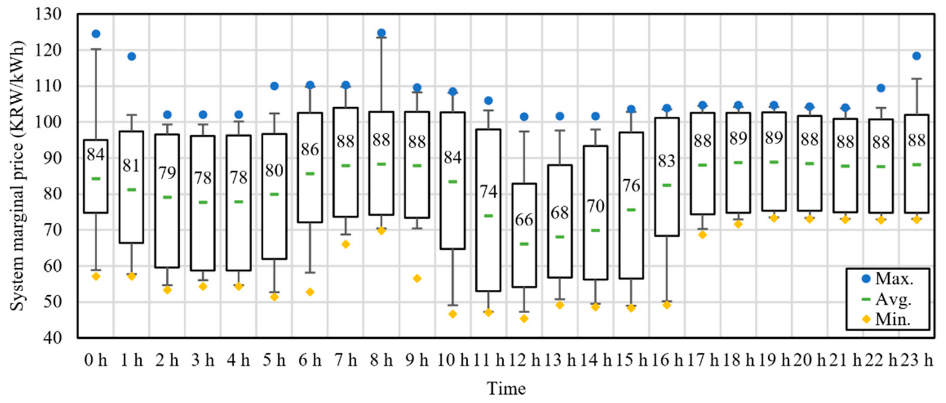
Figure 4 shows the distribution of the system marginal price (SMP) that is calculated using the previously defined market setting. Each box ranges from Q1 to Q3, and whiskers denote the 1st and 99th percentiles of SMP. The average SMP for each hour ranges from 66 to 88 KRW/kWh. The average SMP during the daytime is lower than that of other times because the net demand is low during the daytime (11 h to 15 h). In addition, the average SMP prices are also high during the morning and evening hours when net demand is also high.
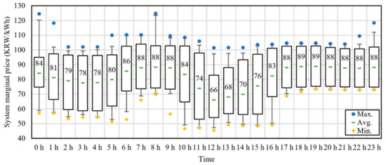
Figure 4.
Representative values of system marginal price obtained from market simulation.
4.3. Imbalance Settlement Simulation Settings
To compare the imbalance pricing formulated in Section 3, a total of six experimental groups are presented, and the summarized features of each group are shown in Table 3. In Cases I, IV, and V, the direction of the imbalances is not considered in the imbalance pricing; that means, whether an imbalance of a VRE worsens the system imbalance or not, the imbalance prices for both directions are the same. On the other hand, in Cases II and III, imbalance prices get penalties when one’s imbalance increases the system imbalance. In Case I and undersupply case of Cases IV and V, thresholds are not considered, because there are no penalties for those cases. In Case II, the threshold is not considered, because the penalty on the price only depends on the direction of imbalance. In other cases, thresholds are applied to relieve the penalties.
Table 3.
Summary of each pricing case.
A basic study is conducted to compare the revenue of the defined groups in each case. Furthermore, a further study is conducted in Case III, which focuses on the incentives for the forecast accuracy of VREs. The parameter values for each study are provided in Table 4 and Table 5, respectively.
Table 4.
Parameters in basic study.
Table 5.
Parameters in each scenario.
5. Simulation Results
5.1. Basic Study: Comparison of Revenue among the VRE Groups
The average revenue of each group is compared for each pricing case. The total settlement of each VRE, which is the sum of the DAM settlement, RTM settlement, and imbalance settlement, is calculated using the DAM price and RTM price.
Figure 5 shows the relative value of each PV group’s average revenue versus the result in the reference case. In the reference case, all PV groups have the same revenue of KRW 2024 million (approximately USD 1.7 million). In the reference case, the output of each time is settled at the previous day’s price regardless of the output prediction. In the reference case, each VRE is paid at the DAM price for each hourly output. Because all generators are assumed to have the same hourly output, in the reference case, all generators in all groups have the same settlement results.
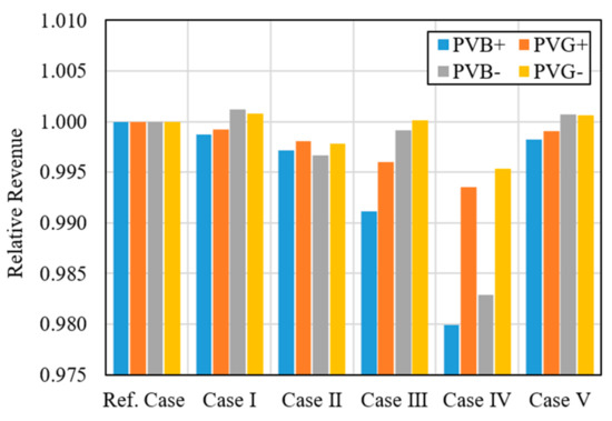
Figure 5.
Average revenue of each PV in each group according to imbalance pricing schemes.
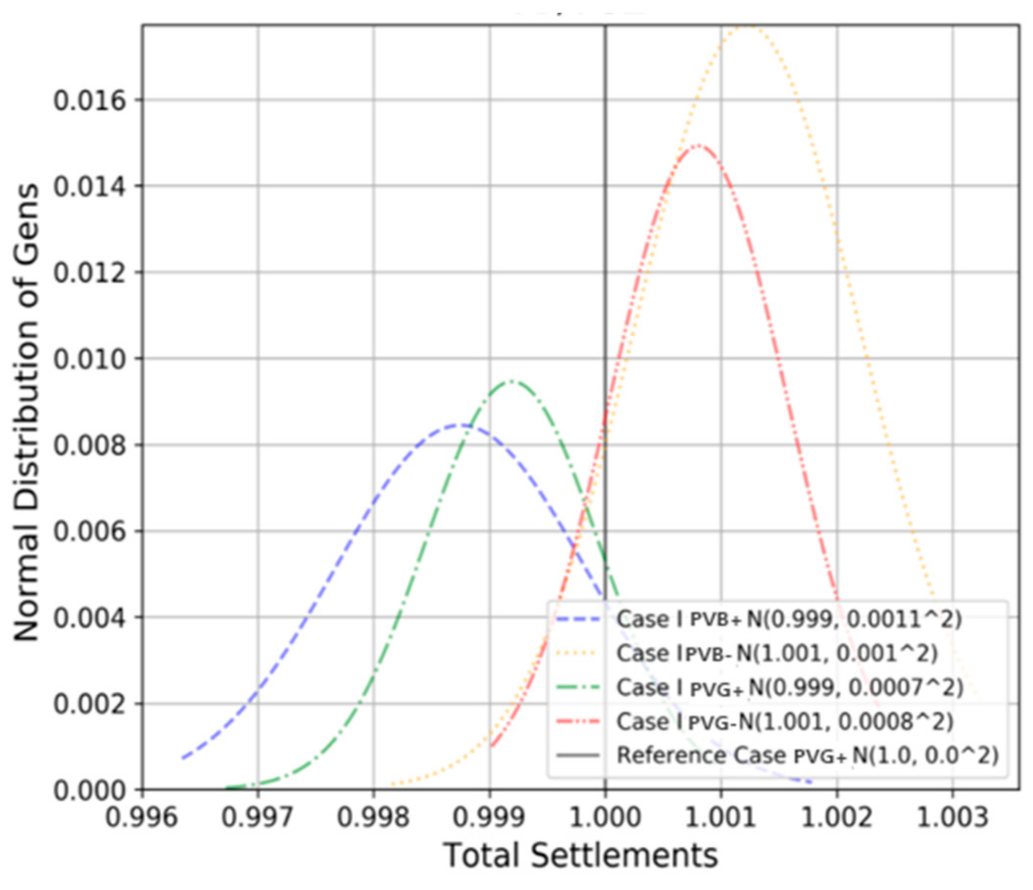
Figure 6 shows the distribution of the revenue of each PV in each group in Case I, and the solid black vertical line denotes the revenue in the reference case. The average revenue of each group is PVB- > PVG- > reference case > PVG+ > PVB+. This is because the groups whose imbalances decrease the system imbalance prefer the RTM price against the DAM price. On the other hand, groups whose imbalances decrease the system imbalance prefer the DAM price against the RTM price. This is furthered in the comparison of PVB- and PVG-, groups that reduce more system imbalance earn more revenue, and similar in the comparison between PVB+ and PVG+, groups that increase more system imbalance earn less revenue.
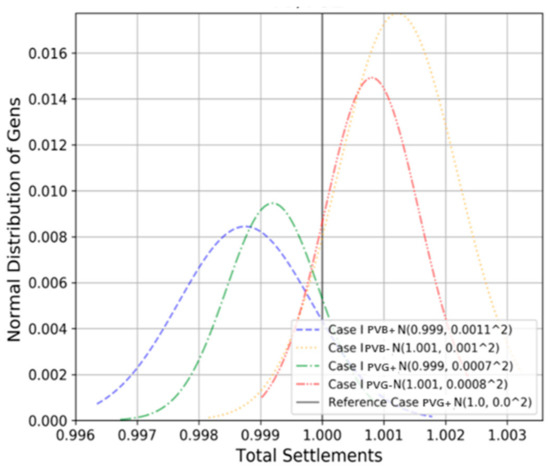
Figure 6.
Distribution of PVs revenue in each group under Case I.
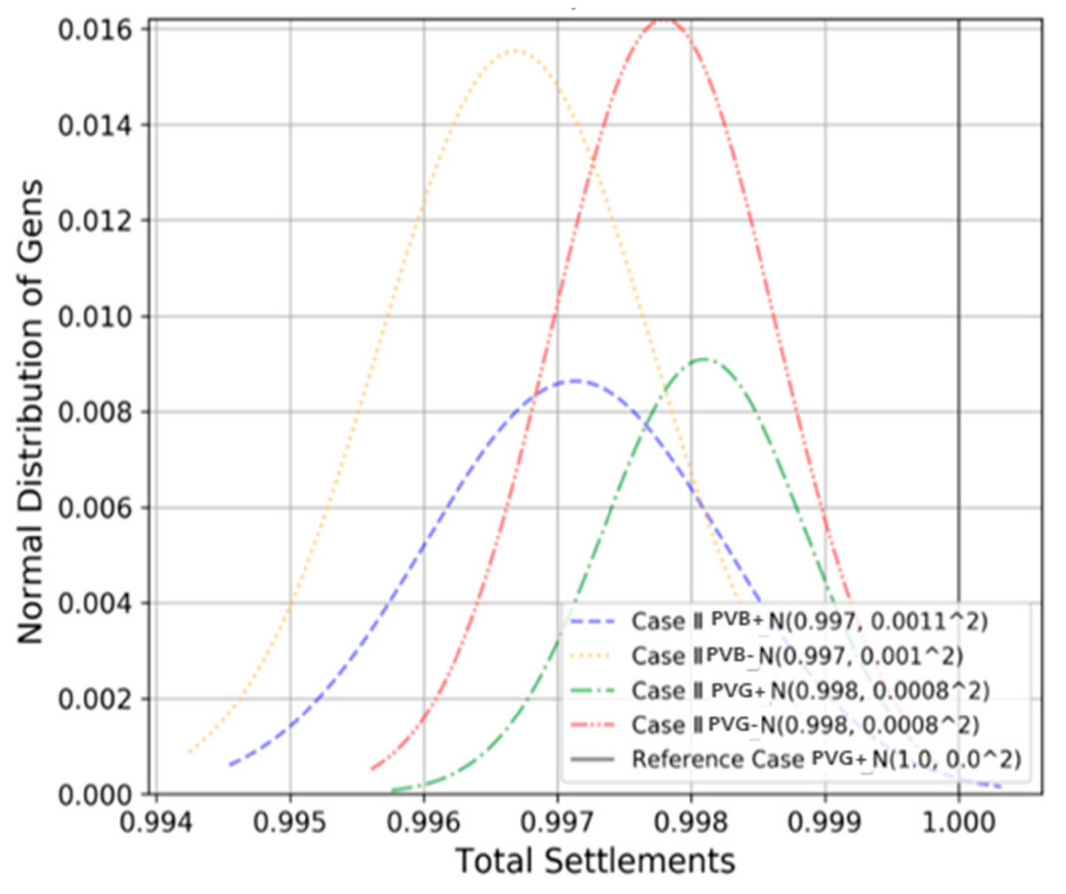
Figure 7 shows the revenue distribution of PV groups in Case II. The revenue in the reference case is larger than any other group, followed by PVG+, PVG-, PVB+, and PVB-. As shown in Case I, the imbalance of aggrading PV groups (PVG+, PVB+) is settled at an unfavorable RTM price. In Case I, the non-aggravating PV groups (PVG-, PVB-) receive greater revenue than the reference case. However, in Case II, there is a penalty for non-aggravating PV groups (PVG-, PVB-) to settle at an unfavorable price among the DAM and RTM prices. Therefore, PVG- and PVB- cannot obtain a higher settlement than the reference case.
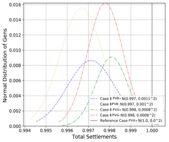
Figure 7.
Distribution of PVs revenue in each group under Case II.
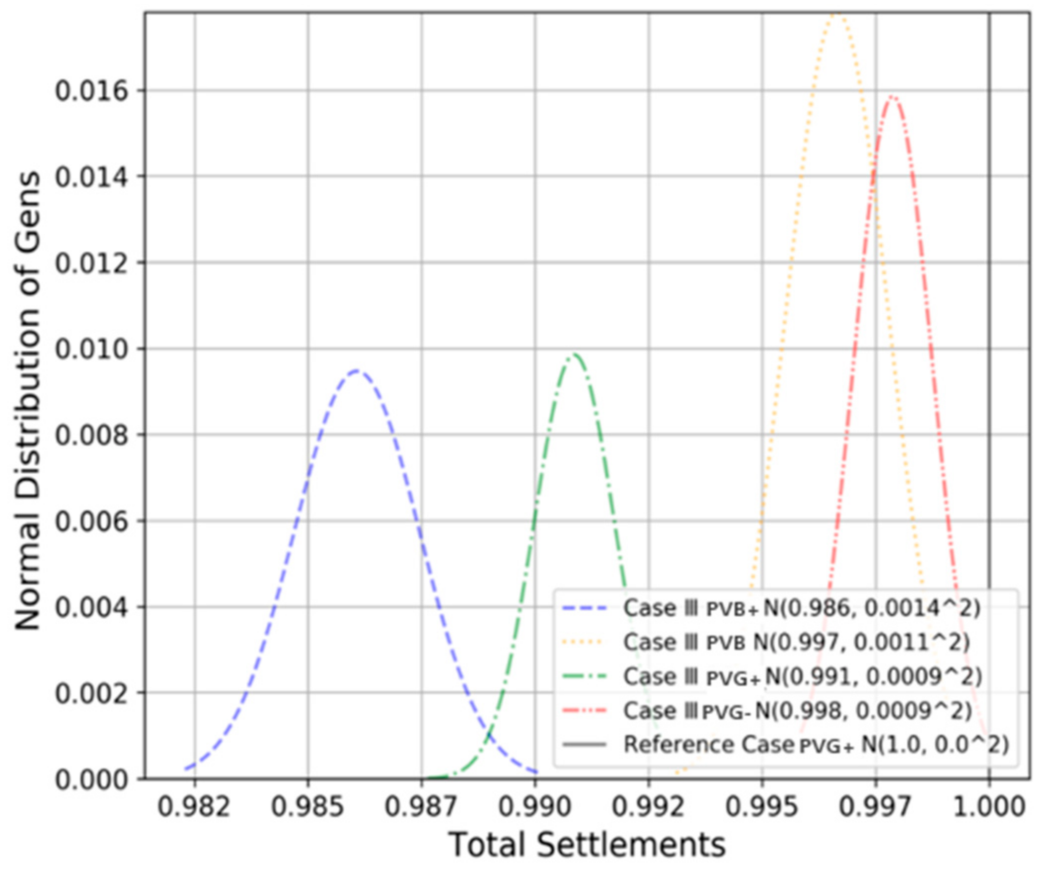
Figure 8 shows the revenue distribution of PV groups in Case III. The average revenues of PVB+ and PVG+ are significantly lower than those of PVB- or PVG-. This is because, in Case III, the penalty price is applied to the aggravating groups when their imbalance exceeds the threshold. In addition, because the forecast error of PVB+ is larger than that of PVG+, PVB+ obtains less profit than PVG+.
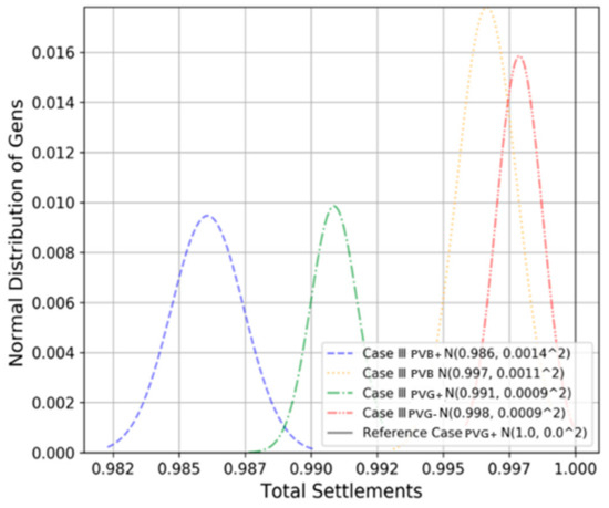
Figure 8.
Distribution of PVs revenue in each group under Case III.
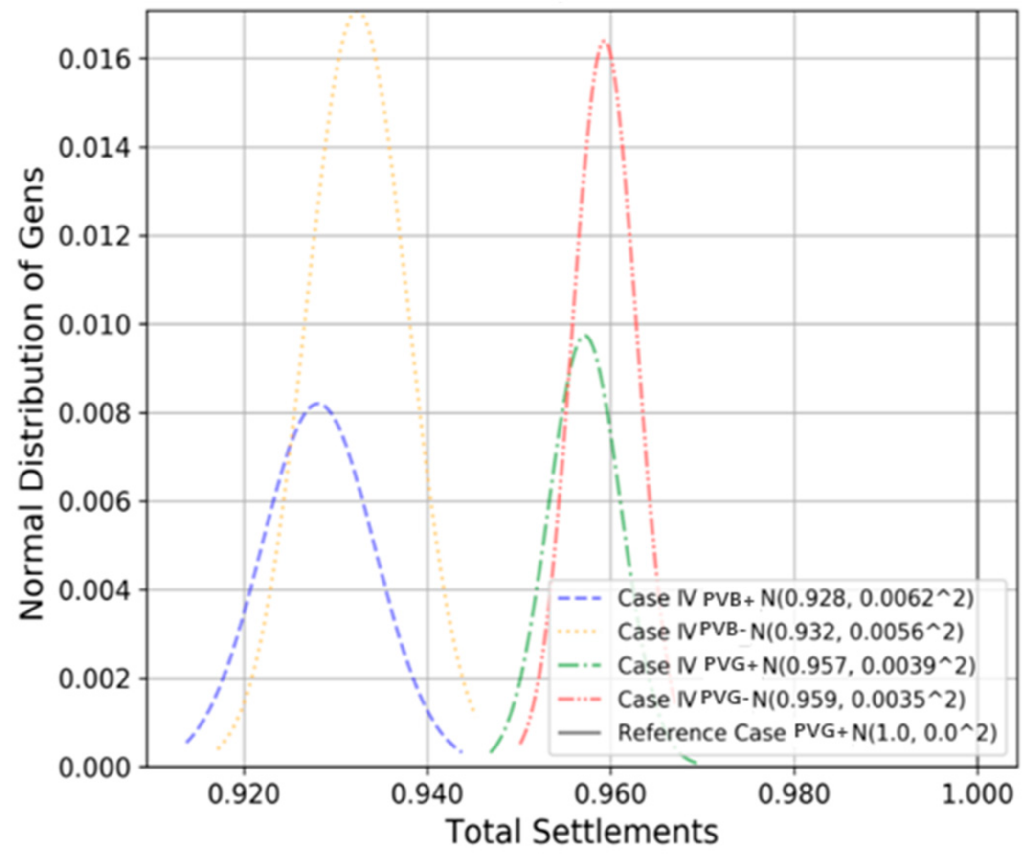
Figure 9 shows the revenue distribution of each PV group in Case IV. The average profits of the inaccurate forecasting groups (PVB+, PVB-) are very low compared to those of the accurate forecasting groups (PVG+, PVG-). In this case, the oversupply above the threshold is not paid, and therefore, the accuracy of the forecast is a major factor that affects the average profit for each group. The rule of not paying for excessive oversupply is a rule aimed at conventional generators. If the rule is applied to VRE, the VRE is intended to over-forecast to avoid oversupply.

Figure 9.
Distribution of PVs revenue in each group under Case IV.
The revenue distribution of each PV group in Case V is shown in Figure 10. The average profits of all groups are higher in Case V than in Case IV. In addition, because the revenue of non-aggravating groups is higher than that of the aggravating groups, the effect of the penalty is reduced in Case V compared to that in Case IV. This is because, unlike Case IV, which did not pay for the imbalance exceeding the threshold, Case V settles at the lower price between the DAM price and RTM price. Specifically, because penalties are not applied to undersupply imbalance, PVG- and PVB- can benefit from the RTM price, which is favorable to them. Similarly, in Case IV, the penalty rule is aimed at conventional generators. Thus, if the rule is applied to VRE, the VRE has an incentive to over-forecast to avoid oversupply.
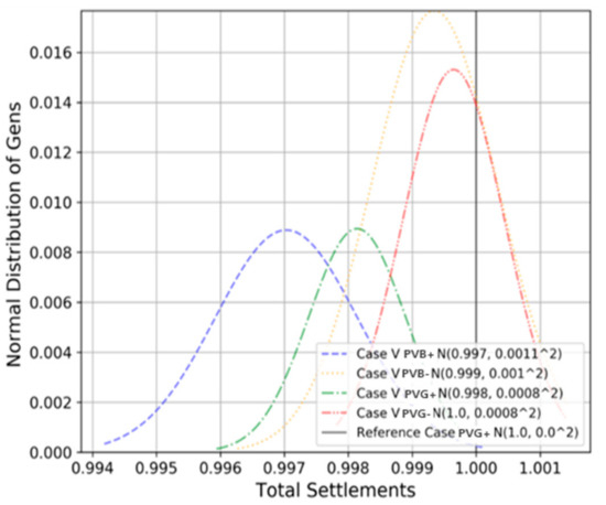
Figure 10.
Distribution of PVs revenue in each group under Case V.
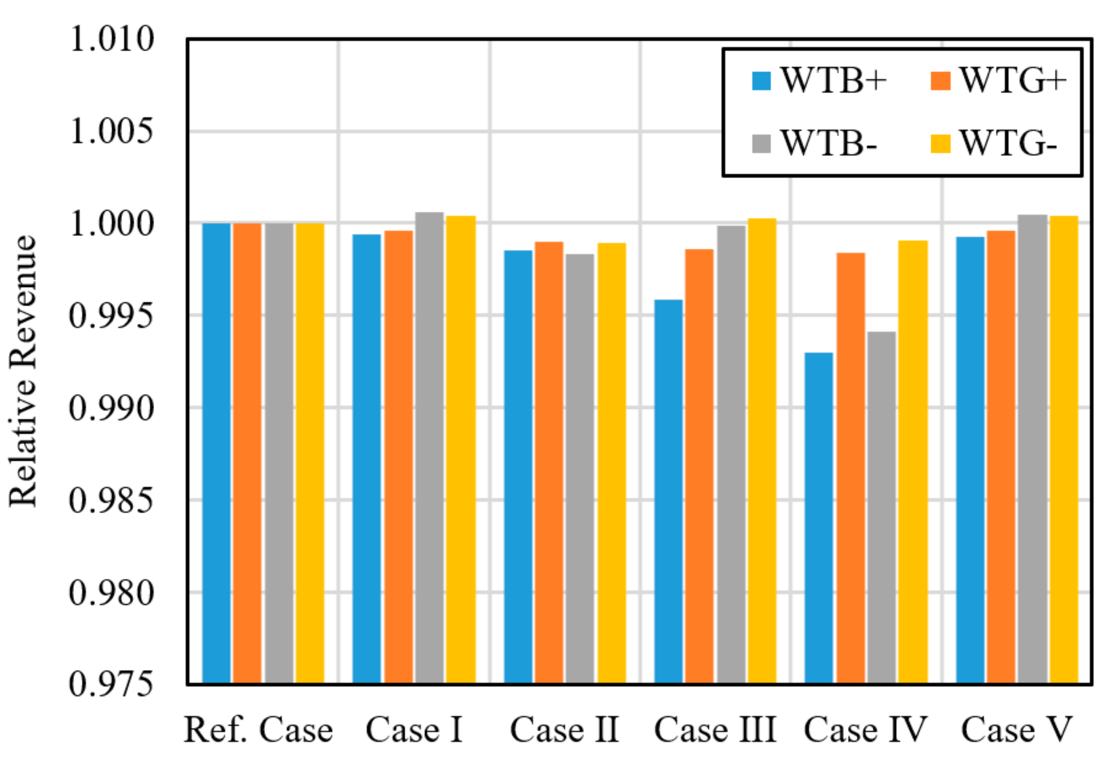
The average revenue of each WT group (WTB+, WTB-, WTG+, and WTG-) in each case is shown in Figure 11. The relative revenue in each case is denoted based on KRW 3691 million (approximately USD 3.1 million), which is the settlement of WT in the reference case. The WT group’s revenue trend in each case shows a similar trend to that of PV groups. However, because it is assumed that the prediction accuracy of the WT groups is higher than that of PVs, the effect of the imbalance on revenue is less; thus, the revenues are closer to 1.

Figure 11.
Average revenue of each WT in each group according to imbalance pricing schemes.
5.2. Comparison of Settlement Results According to the Degree of Imbalance
In the preceding subsection, the revenue for each group was compared for each case. The groups are divided regarding their power source, forecast accuracy, and imbalance direction between system imbalances. However, in the real world, various uncertainty factors exist, and thus, whether a specific generator increases the system imbalance can be determined without any specific tendency. Therefore, PVBavg, PVGavg, WTBavg, and WTGavg are newly defined by considering only the power source and forecast accuracy. The revenue of the average group is the average of that of the aggravating group and that of the non-aggravating group. For example, the settlement of PVBavg is the average of the revenues of PVB+ and PVB-.
The settlement results for each group in all cases are shown in Figure 12. The result of the reference case is set to 1.0, as in the previous case. The revenue of all PV and WT groups in Case I is 1.0. On the other hand, in Case II to Case V, for the PV groups, the revenue of the reference case is followed by PVGavg and PVBavg. This trend is also shown for the WT groups, as the revenue of the reference case is followed by WTGavg and WTBavg. This means that Case I cannot provide the VREs the incentive to improve their forecast accuracy. On the other hand, other cases can provide the VREs the incentives to make accurate predictions, because a more accurate forecast leads to higher revenue.
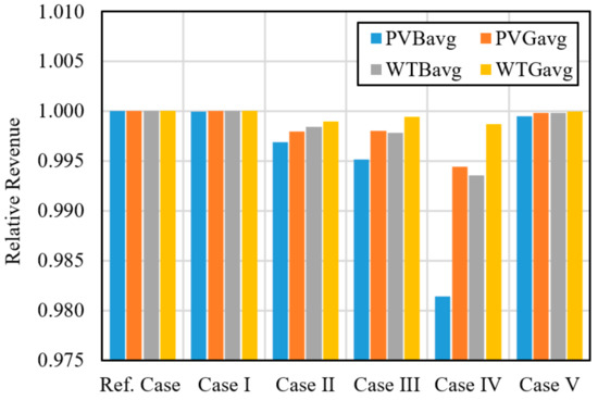
Figure 12.
Average revenue of PVB avg, PVGavg, WTBavg, and WTGavg groups according to imbalance pricing schemes.
In Case II, there are no adjustable parameters for rule-makers to regulate the incentives for reducing forecast errors for each VRE. On the other hand, for Cases III to V, the rule makers can regulate the incentive through the adjustment of the threshold ratio or penalty ratio. In Cases IV and V, the penalty price is applied only when an oversupply imbalance occurs. As noticed previously, these rules have limitations in that they lead the VREs to over-predict. On the other hand, Case III imposes the penalties for both directions and can even adjust the penalty ratio. Therefore, simulations are conducted for Case III under the parameter sets listed in Table 5.
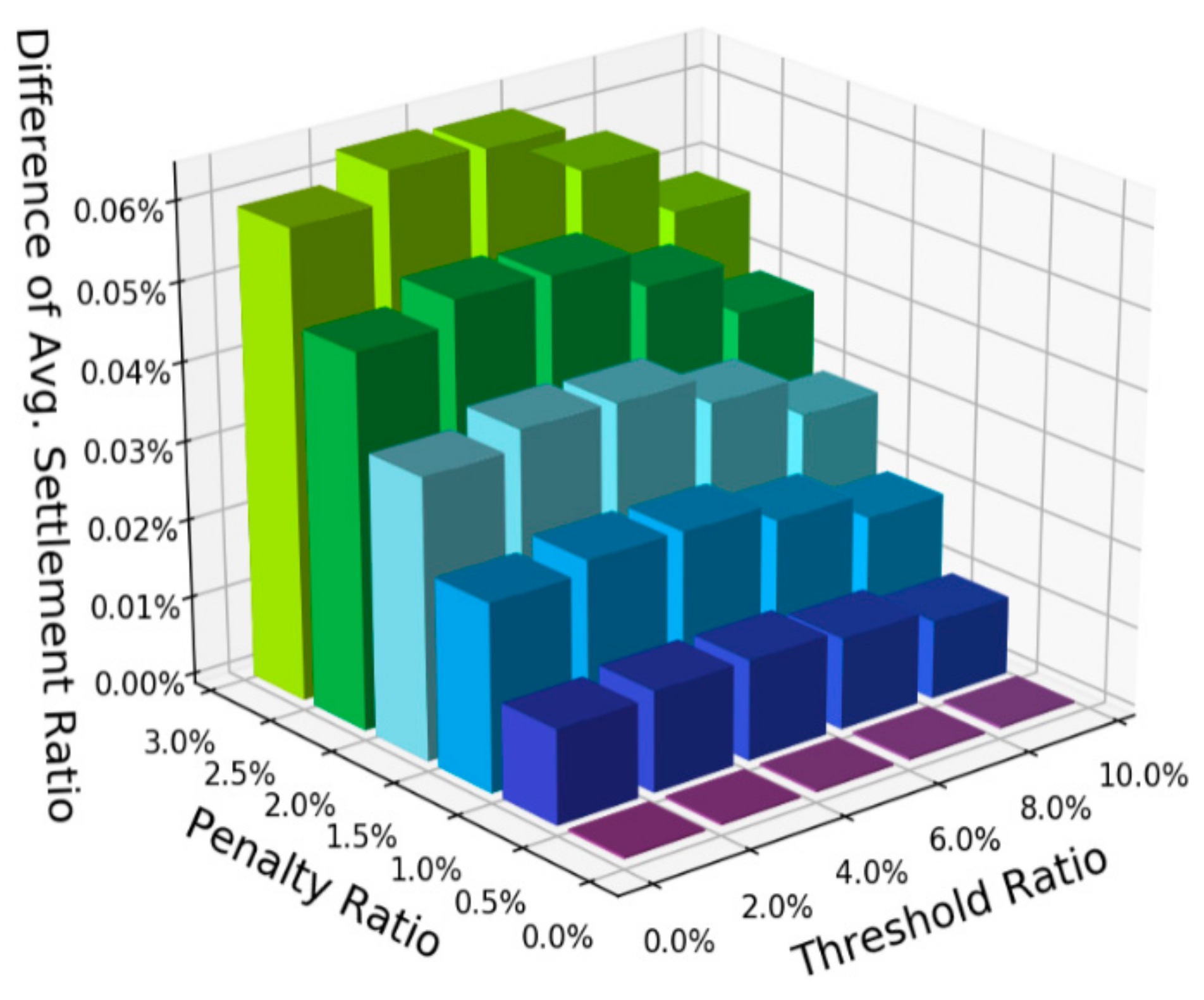
To see the impact of the pricing on the incentive to improve the forecast accuracy., the revenue differences between PVGavg and PVBavg, WTGavg, and WTBavg are compared. As in the previous results, the size of the settlement in the reference case is set at 1. Figure 13 shows a graph of the revenue difference between PVGavg and PVBavg under each parameter set. The cases where the penalty ratio is 0 are the same as Case I, which have no differences between the two groups. As the penalty ratio increases, the difference between the two groups (PVGavg–PVBavg) increases linearly. Although the penalty price applied to both groups is the same, the penalty amount applied to PVBavg is larger, and, thus, PVBavg has a lower revenue than PVGavg.

Figure 13.
Average revenue of each PV in each group according to imbalance pricing schemes.
The mean of PVGavg’s RTM error is 5.6%, and that of PVBavg’s RTM error is 8.4%. As the threshold ratio increases to 8%, the difference in revenues also increases, because the imbalances included in the threshold ratio are more in PVGavg than in PVBavg. However, as the threshold ratio exceeds 8%, the difference in revenues slightly decreases, because the imbalances newly included in the threshold ratio are higher in PVBavg compared with PVGavg.
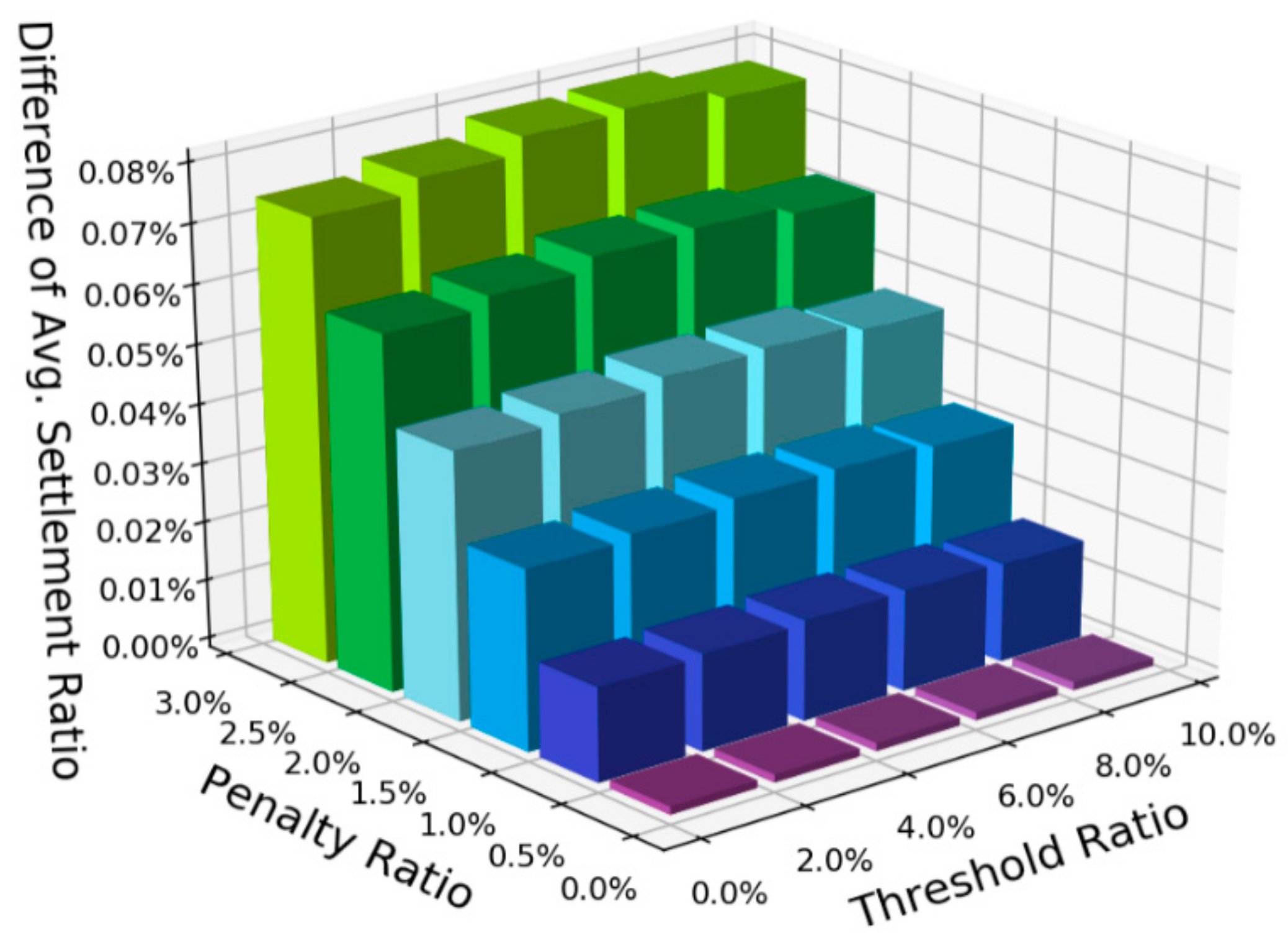
This trend is more prominent in the case of the WT groups, as shown in Figure 14. The trend regarding the penalty rate is similar to that of the PV groups. However, regarding the threshold ratio, the point at which WTGavg–WTBavg decreases is between 6% and 8%, which is between 8% and 10% in the PV group. This is because the mean of the WTGavg’s RTM error is 4.5%, and that of the WTBavg’s RTM error is 6.7%. By adjusting the penalty ratio and the threshold ratio, the rule maker can adjust the incentives for the groups with different forecast errors.

Figure 14.
Average revenue of each WT in each group according to imbalance pricing schemes.
5.3. Results Summary
For PVB+ and PVG+, the reference case is the best option, followed by Cases I, V, II, III, and IV. For PVB- and PVG-, Case I is the best option, followed by Case V, the reference case, Case III, Case II, and Case IV. In Cases II and V, PVB- and PVG- earn greater revenue compared to the reference case. Case IV is harsher than any other case, because all the groups earn the lowest revenue in this case. It is also shown that these trends are similarly shown in the WT groups. From the results of the average groups, Cases II, III, IV, and V can give differences in the revenue according to their size of uncertainties. Among the cases, Case III only imposes the penalties for both directions and can even adjust the penalty ratio. In Case III, further results comparing the revenue differences between PVGavg and PVBavg and between WTGavg and WTBavg show that the rule-maker can target the exemption groups and adjust the intensity of the incentives.
6. Discussion
6.1. Type I: Not Effective in Reducing the System Imbalance Compared to Other Cases
The results presented in Figure 5, Figure 6, and Figure 11 show that Case I can encourage the VREs to make imbalances in the direction that reduces the system imbalance. However, for the VREs of which the imbalances are not intended but inevitable, the imbalance in real world will be more similar to the results presented in Figure 12. Figure 12 shows that Type I cannot give incentives for the VREs to predict more accurately. Figure 6 shows that a higher imbalance leads to a higher risk of VRE revenue. Thus, Type I may encourage the VREs to increase their forecast accuracy to some extent but as much as other types of imbalance pricing schemes.
6.2. Type IV and V: Not appropriate for the VREs
In Cases IV and V, the penalty prices are only applied to oversupply imbalances. These rules are designed to apply to traditional generators. The purpose was to prevent obtaining excess profits from intentional oversupply imbalances and reduce the uncertainties in the system. As shown in the simulations, if these rules are applied to VREs as they are, VREs have an incentive to overestimate their output forecasts. This is because it is more advantageous for the VREs to be settled at the RTM price instead of penalty prices. Therefore, there are limitations to apply these rules to the VREs. Therefore, if the regulator uses imbalance pricing to increase the accuracy of VRE, Type II or Type III is more effective than Type IV or Type V.
6.3. Type III: A Nice Tool for the Regulators to Encourage More Accurate Forecasts
Because imbalance settlement pricing can give penalties to VREs that are bad at forecasts, it can be used as a means of encouraging the development of forecasting technology. However, despite advances in forecasting technologies, there will inevitably be errors in the forecasts under the rule that the forecasts are submitted before the real-time. If the threshold size is set below the technically achievable error level, the VREs will be excessively penalized. Therefore, it is necessary to set the threshold size at or a little higher than the technically achievable error level. Even though the threshold is equal to or greater than the mean value of the technically achievable level of error, the forecast error rate appears as a probabilistic distribution, which can motivate advances in forecasting technologies.
In Figure 14, with the same penalty ratio, when the threshold ratio is 6%, that is, between WTGavg’s RTM error (4.5%) and WTBavg’s RTM error (6.7%), the revenue between the two groups is the largest. This result is because most imbalances of WTGavg are not subject to penalty, and most imbalances of WTBavg are subject to penalty. The VREs with the forecast errors smaller than the threshold ratio will be less affected by the penalty than the VREs with the forecast errors bigger than that. Furthermore, by adjusting the penalty ratio, the regulators can adjust the intensity of incentives for the groups with different forecast errors.
7. Conclusions and Policy Implications
The increase in VRE will increase the uncertainty in the power system and power market and increase the balancing cost. Therefore, it is necessary to incentivize the VREs to reduce the uncertainty from their output. An imbalance settlement is one of the policy tools that can lead the VREs to reduce their imbalances by increasing their prediction accuracy. Previous studies only compared the effect of pricing schemes on single or a few VREs, which was not sufficient to figure out the impact of pricing schemes on VREs with different forecast accuracies including the risks. In this study, multiple VREs are defined, and the impacts of each pricing type on each VRE group are compared. Through the methodology used in this study, it is possible to analyze whether the regulators can give incentives to the potential VRE investors.
The current Korean electricity market has limitations, such as the absence of a price that reflects the real-time value and the lack of incentives to submit accurate forecasts by VREs. To overcome these limitations, the ISO announced a plan to introduce the RTM, which is denoted as Type I. However, the effectiveness of the introduction regarding the incentive on the VREs seems limited. The result shows that Type I pricing on the imbalance does not make a difference in the revenues of VRE groups with different forecast accuracies. On the other hand, Types II–V can provide an incentive to the VRE groups. However, it is difficult for the rule maker to adjust the intensity of incentives in Type II. In Types IV and V, the VREs are prone to submitting overestimated forecasts.
In contrast, the Type III benchmarking pro forma OATT is demonstrated as a useful settlement rule. Type III can determine the difference in revenue between the groups with different forecast accuracies by adjusting two parameters: the penalty ratio and threshold ratio. The increase in the penalty leads to a larger gap in revenues between the groups. The larger the difference, the greater the incentive for accurate predictions. However, the difference decreases when the threshold ratio passes the mean of the bad forecasting group’s forecast error. The results confirm that the difference in incentives for accurate forecasts can be adjusted by adjusting the penalty ratio and the threshold ratio. The introduction of the imbalance settlement has an impact on the profitability of VRE and is, therefore, dependent on policy judgment by regulatory authorities. However, in the process of introducing RTM, it is possible to create an imbalance settlement that includes sufficient exemptions for the VREs. By creating rules that include sufficient exemptions, regulators can provide VREs ample time to invest in forecasting and control technologies. In the future, as the VREs reach grid parity, it is expected that practical application will be possible by gradually activating the rules.
Author Contributions
Conceptualization, Y.Y. and S.K.; methodology, H.M. and S.K.; software, D.L., J.H., and H.M.; investigation, D.L. and J.H.; writing—original draft preparation, H.M.; writing—review and editing, S.K.; visualization, D.L.; supervision, S.K.; project administration, Y.Y. and S.K.; funding acquisition, S.K. All authors have read and agreed to the published version of the manuscript.
Funding
This research received no external funding.
Institutional Review Board Statement
Not applicable
Informed Consent Statement
Not applicable
Acknowledgments
This work has been financially supported by the R&D project of Korea Power Exchange, which has a title of “A feasibility study of the imbalance settlement according to the increase in variable renewable energy”.
Conflicts of Interest
The authors declare that they have no known competing financial interests or personal relationships that could have appeared to influence the work reported in this paper.
References
- Murdock, H.E.; Gibb, D.; André, T.; Appavou, F.; Brown, A.; Epp, B.; Sawin, J.L. Renewables 2019 Global Status Report; REN 21: Paris, France, 2019. [Google Scholar]
- 3020 Renewable Energy Plan; Ministry of Trade, Industry, and Energy (MOTIE): Sejong, Korea, 2017. Available online: http://www.motie.go.kr/motiee/presse/press2/bbs/bbsView.do?bbs_seq_n=159996&bbs_cd_n=81 (accessed on 3 June 2021).
- Jónsson, T.; Pinson, P.; Madsen, H. On the market impact of wind energy forecasts. Energy Econ. 2010, 32, 313–320. [Google Scholar] [CrossRef] [Green Version]
- Goodarzi, S.; Perera, H.N.; Bunn, D. The impact of renewable energy forecast errors on imbalance volumes and electricity spot prices. Energy Policy 2019, 134, 110827. [Google Scholar] [CrossRef]
- Annual Report on the Results of Monitoring the Internal Electricity and Natural Gas Markets in 2017—Electricity Wholesale Markets Volume. 2018. Available online: https://www.acer.europa.eu/Official_documents/Acts_of_the_Agency/Publication/MMR%202017%20-%20ELECTRICITY.pdf (accessed on 3 June 2021).
- Herrero, I.; Rodilla, P.; Batlle, C. Enhancing intraday price signals in us iso markets for a better integration of variable energy resources. Energy J. 2018, 39. [Google Scholar] [CrossRef]
- Karanfil, F.; Li, Y. The role of continuous intraday electricity markets: The integration of large-share wind power generation in Denmark. Energy J. 2017, 38. [Google Scholar] [CrossRef]
- Hodge, B.M.; Florita, A.; Sharp, J.; Margulis, M.; Mcreavy, D. Value of Improved Short-Term Wind Power Forecasting; (NREL/TP-5D00-63175); National Renewable Energy Laboratory (NREL): Golden, CO, USA, 2015. [Google Scholar]
- Kirschen, D.S.; Strbac, G. Fundamentals of Power System Economics; John Wiley and Sons: Hoboken, NJ, USA, 2018. [Google Scholar]
- De Vos, K.; Driesen, J.; Belmans, R. Assessment of imbalance settlement exemptions for offshore wind power generation in Belgium. Energy Policy 2011, 39, 1486–1494. [Google Scholar] [CrossRef]
- Wan, Y.H.; Milligan, M.; Kirby, B. Impact of Energy Imbalance Tariff on Wind Energy; (NREL/CP-500-40663); National Renewable Energy Laboratory (NREL): Golden, CO, USA, 2007. [Google Scholar]
- Brunetto, C.; Tina, G. Wind generation imbalances penalties in day-ahead energy markets: The Italian case. Electr. Power Syst. Res. 2011, 81, 1446–1455. [Google Scholar] [CrossRef]
- Chaves-Ávila, J.P.; Hakvoort, R.A.; Ramos, A. The impact of European balancing rules on wind power economics and on short-term bidding strategies. Energy Policy 2014, 68, 383–393. [Google Scholar] [CrossRef]
- Haring, T.W.; Kirschen, D.S.; Andersson, G. Incentive compatible imbalance settlement. IEEE Trans. Power Syst. 2015, 30, 3338–3346. [Google Scholar] [CrossRef]
- Wu, Z.; Zhou, M.; Zhang, T.; Li, G.; Zhang, Y.; Liu, X. Imbalance settlement evaluation for China’s balancing market design via an agent-based model with a multiple criteria decision analysis method. Energy Policy 2020, 139, 111297. [Google Scholar] [CrossRef]
- Alexander, G.J.; Baptista, A.M. A comparison of VaR and CVaR constraints on portfolio selection with the mean-variance model. Manag. Sci. 2004, 50, 1261–1273. [Google Scholar] [CrossRef] [Green Version]
- Ahlqvist, V.; Holmberg, P.; Tangerås, T. Central-versus Self-Dispatch in Electricity Markets. SSRN Electr. J. 2018, 1257. [Google Scholar] [CrossRef] [Green Version]
- Song, Y.; Kim, H.; Kim, S.; Jin, Y.; Yoon, Y. How to find a reasonable energy transition strategy in Korea? Quantitative analysis based on power market simulation. Energy Policy 2018, 119, 396–409. [Google Scholar] [CrossRef]
- The Manual of Korean Power Market Operation; Korea Power Exchange (KPX): Naju-si, Korea, 2020. Available online: https://www.kpx.or.kr/www/selectBbsNttView.do?key=29&bbsNo=114&nttNo=20914&searchCtgry=&searchCnd=all&searchKrwd=&pageIndex=1&integrDeptCode (accessed on 3 June 2021).
- Ela, E.; Milligan, M.; Bloom, A.; Botterud, A.; Townsend, A.; Levin, T. Evolution of Wholesale Electricity Market Design with Increasing Levels of Renewable Generation; (NREL/TP-5D00-61765); National Renewable Energy Laboratory (NREL): Golden, CO, USA, 2014. [Google Scholar]
- Commission Regulation (EU) 2017/2195 Establishing a Guideline on Electricity Balancing (Text with EEA Relevance); European Commission: Brussels, Belgium, 2017. Available online: https://eur-lex.europa.eu/legal-content/EN/TXT/?uri=CELEX%3A32017R2195 (accessed on 3 June 2021).
- Imbalance Pricing Guidance: A Guide to Electricity Imbalance Pricing in Great Britain; Elexon: London, UK, 2016. Available online: https://www.elexon.co.uk/documents/training-guidance/bsc-guidance-notes/imbalance-pricing/ (accessed on 3 June 2021).
- Manual 28: Operating Agreement Accounting (Revision 82); PJM: Norristown, PA, USA, 2019. Available online: https://www.pjm.com/-/media/documents/manuals/archive/m28/m28v82-operating-agreement-accounting-07-25-2019.ashx (accessed on 3 June 2021).
- Nordic TSOs Discussion Paper on Imbalance Pricing; Nordic Balancing Model (NBM); Svenska Kraftnät: Sundbyberg, Sweden, 2019. Available online: https://nordicbalancingmodel.net/wp-content/uploads/2019/11/Discussion-paper-on-imbalance-pricing.pdf (accessed on 3 June 2021).
- All TSOs’ Proposal to Further Specify and Harmonise Imbalance Settlement in Accordance with Article 52(2) of the Commission Regulation (EU) 2017/2195 of 23 November 2017 Establishing a Guideline on Electricity Balancing; ENTSO-E: Brussels, Belgium, 2018. Available online: https://eepublicdownloads.blob.core.windows.net/public-cdn-container/clean-documents/nc-tasks/EBGL/EB GL_A52.2_191030_All_TSOs_ISHP_imbalance_settlement_harmonisation_amended_proposal_for_submission.pdf (accessed on 3 June 2021).
- FERC Order 888; FERC: Washington, DC, USA, 1996. Available online: https://www.ferc.gov/industries-data/electric/industry-activities/open-access-transmission-tariff-oatt-reform/history-oatt-reform/order-no-888 (accessed on 3 June 2021).
- FERC Order 890; FERC: Washington, DC, USA, 2007. Available online: https://www.ferc.gov/sites/default/files/2020-05/E-1fr890.pdf (accessed on 3 June 2021).
- Accounting and Billing Manual; NYISO: New York, NY, USA, 2020. Available online: https://www.nyiso.com/documents/20142/2923231/acctbillmnl.pdf/ (accessed on 3 June 2021).
- Post Operating Processor 5 Minutes Calculation Guide; MISO: Carmel, IN, USA, 2020. Available online: https://cdn.misoenergy.org/POP%20Guide%20Changes%20-%20MRD%20FERC%20205%20filing%20Docket%20No.%20ER21-239-000490698.pdf (accessed on 3 June 2021).
- Market Settlements 5 Minutes Calculation Guide; MISO: Carmel, IN, USA, 2020. Available online: https://www.misoenergy.org/markets-and-operations/notifications-overview/market-settlements-notifications/5-minute-settlements/ (accessed on 3 June 2021).
- The 8th the Electricity Supply and Demand Plan (ESDP); Korea Power Exchange (KPX): Naju-si, Korea, 2017. Available online: https://www.kpx.or.kr/www/contents.do?key=92 (accessed on 3 June 2021).


Publisher’s Note: MDPI stays neutral with regard to jurisdictional claims in published maps and institutional affiliations. |
© 2021 by the authors. Licensee MDPI, Basel, Switzerland. This article is an open access article distributed under the terms and conditions of the Creative Commons Attribution (CC BY) license (https://creativecommons.org/licenses/by/4.0/).