Validation of Modified Algebraic Model during Transitional Flow in HVAC Duct

Abstract

Airflow occurring in a ventilation duct is characterized by low velocity and hence low Reynolds number. In these conditions, either a laminar, transitional or turbulent flow will occur. Different flow conditions result in different values of the friction coefficient. To achieve the transitional flow in numerical simulation, a modified algebraic model for bypass transition (modified $k-\omega$) was used. Numerical simulation was validated using Particle Tracking Velocimetry (PTV) in the circular channel. The modified algebraic model consists of only two partial differential equations, which leads to much faster calculation than the shear stress transport model. Results of the modified algebraic model are largely consistent with either the measurement and shear stress transport model considering laminar and transitional flow. Consistency slightly decreased in turbulent flow in relation to the model using shear stress transport method.

1. Introduction

One of the elements of the heat ventilation and air condition (HVAC) system design is to determine the ventilation duct velocity. To achieve this part of design, computational fluid mechanics (CFD) are used [1]. However, CFD in HVAC mainly is used to determine flow parameters in a specific room, not the ventilation duct [2,3,4]. Airflow velocity in HVAC system is one of the most important parameters of the HVAC system, which determines the comfort of room inhabitants, i.e., thermal comfort [4,5], CO${}_2$ concentration [3]. Flow through HVAC ducting system also consumes energy and it is crucial to balance the comfort and energy consumed by the system, especially when automatic control is applied [6].

In this paper, the authors propose a modified turbulence model applied in CFD simulation to determine the channel velocity profile for model validation by measuring specific velocity profiles in a circular channel with steady flow. Airflow through the ventilation duct characterizes with low velocity [3], which induces low Reynolds Number. At low Reynolds number, the flow can be either laminar, transitional, or turbulent [7,8]. This leads to differences between the flow friction factor and energy losses during the flow through channel. Different friction factor leads also to different heat transfer coefficient [9]. Errors induced by the poor choice of CFD modelling method may have an influence on the simulations of the recuperator, where heat exchange occurs in a gaseous medium.

There are many numerical models to simulate transitional flows available today. There is a set of models based on Reynolds Average Simulation (RAS), models based on Large Eddy Simulation (LES) and Direct Numerical Simulation (DNS). DNS is the most accurate model, but is very time consuming. LES are less accurate but also less time consuming [10]. The fastest are RAS, but is accuracy depends on case. In laminar flow simulations are relatively easy to perform, for turbulent flow when using RAS, there are a set of models that solve turbulence. The most popular turbulence model is $k-\omega SST$ [11]. For simulating the transitional flow between laminar and turbulent, there is no universal model. The transitional flow can be simulated with, for example, LOTRAN package which is part of the commercial software ANSYS [12]. In the literature, there are comparisons of different RAS models for transitional flow [13]. In the paper, there are results for Spalart-Allmaras, low-Re $k-ϵ$, Re-Normalisation Group (RNG), Low-Re Shear Stress Transport, $k-\omega SST$, and V-SA [14] model. The comparisons shows that for transitional flow the best result are obtained with $k-\omega SST$ and V-SA model. Recently, for the transitional flow was proposed modified model based on standard $k-\omega$ [15,16,17]. The model proposed in [15] was originally developed for turbomachinery, the model from [17] is for flow around airfoils. Only model proposed in [16] which is a modification of [15] model can be applied for internal duct flow, however it was validated only with literature data, not in particular for HVAC ducts. Therefore, in this paper, a validation of this model is performed using PTV measurement method.

The model presented in this work is an algebraic turbulence model based on the standard $k-\omega$ [18,19]. Algebraic model was originally developed in [15]. Because this algebraic model was developed for high Reynolds number flow, a modification proposed in [20] was applied.

To validate the algebraic model used in this work, a measurement using particle tracking velocimetry (PTV) was used. This method is widely used in the measurement of velocity field in fluids and in validate the numerical simulation results [21,22,23,24,25].

2. Governing Equations

The numerical model used in this study for describing statistically steady fluid flow contains a system of partial differential equations. These equations represent the mass and momentum balance. Balance equation system includes the continuity equation and Reynolds-averaged Navier-Stokes equations (RANS) [16]:

$$\frac{\partial u_j}{\partial x_j}=0,$$

(1)

$$\rho \left(\frac{\partial }{\partial x_j}{u}_j{u}_i\right)=-\frac{\partial p}{\partial x_i}+\frac{\partial }{\partial x_j}\left(t_{ij}+\rho {\tau }_{ij}\right)i,j=1,2,3.$$

(2)

Tensor components $t_{ij}$ and ${\tau }_{ij}$ are determined by:

$$t_{ij}=2\rho \nu S_{ij},\rho {\tau }_{ij}=2\rho {\nu }_t{S}_{ij}-\frac{2}{3}\rho k{\delta }_{ij},$$

(3)

$$S_{ij}=\frac{1}{2}\left(\frac{\partial u_i}{\partial x_j}+\frac{\partial u_j}{\partial x_i}\right)-\frac{1}{3}\frac{\partial u_k}{\partial x_k}{\delta }_{ij}.$$

(4)

The algebraic turbulence model used for simulation in this study is a modified $k-\omega$ model formulated in [15]. It bases on the standard $k-\omega$ model by Wilcox [18,19]. New model developed in [15] was originally implemented in FLUENT commercial CFD framework. This model introduce factor $\gamma$ which is a multiplier of the production term in the k-equation. As shown in [15,16,20,26] it enables more accurate description of the flow in the laminar, transitional, and turbulent range. The k and $\omega$ equations are defined:

$$\rho \frac{\partial }{\partial x_j}\left(u_{j}k\right)=\rho \gamma {\nu }_s{S}^2-\rho {\beta }^{\ast }k\omega +\rho \frac{\partial }{\partial x_j}\left[\left(\nu +{\sigma }^{\ast }\frac{k}{\omega }\right)\frac{\partial k}{\partial x_j}\right],$$

(5)

$$\rho \frac{\partial }{\partial x_j}\left(u_j\omega \right)=\rho \alpha \frac{\omega }{k}{\nu }_s{S}^2-\rho \beta {\omega }^2+\rho \frac{\partial }{\partial x_j}\left[\left(\nu +\sigma \frac{k}{\omega }\right)\frac{\partial \omega }{\partial x_j}\right]+\rho \frac{{\sigma }_d}{\omega }\frac{\partial k}{\partial x_j}\frac{\partial \omega }{\partial x_j},$$

(6)

where:

$${\nu }_t={\nu }_s+{\nu }_l,{\nu }_s=\frac{k_s}{{\tilde{\omega }}_1},{\nu }_l=\frac{k_l}{{\tilde{\omega }}_2},k_s=f_{ss}k,k_l=k-k_s,$$

(7)

$${\tilde{\omega }}_1=\max \left[\omega ,C_{lim}\frac{\sqrt{2S_{ij}{S}_{ij}}}{a_1}\right],{\tilde{\omega }}_2=\max \left[\omega ,C_{lim}\frac{\sqrt{2S_{ij}{S}_{ij}}}{a_2}\right],$$

(8)

$$f_{ss}=\exp \left[-{\left(\frac{C_{SS}\nu \mathsf{\Omega }}{k}\right)}^2\right].$$

(9)

The factor $\gamma$ (intermittency factor) is a multiplier of the production term in k-Equation (5). It is defined as:

$$\gamma =\min \left(\frac{{\zeta }_T}{A_T},1\right),{\zeta }_T=\max \left(\frac{\sqrt{k}y}{\nu }-C_T,0\right).$$

(10)

The intermittency factor $\gamma$ can be described as a starting function for the turbulence [15]. When $\gamma =0$ the production term $\rho \gamma {\nu }_s{S}^2$ from Equation (5) is also equals to zero. Therefore there is no production of turbulent kinetic energy $k,$ which corresponds with the laminar flow. For the inlet the assumption of $\gamma =0$ was made. When $0<\gamma <1$ production term has non zero which indicates intermittent flow. The values of $\gamma =1$ leads to fully turbulent flow [16].

Originally, the algebraic intermittency model formulated in [15] was developed to simulate the transition flow in turbomachines. Due to the slightly different flow characteristics in pipes, especially due to different pressure gradient, it was necessary to tune the model constants. As shown in [26], the following model constants shown in

Table 1. Modified constants of algebraic intermittency $k-\omega$ model.

${\mathit{C}}_{\mathit{T}}$	${\mathit{A}}_{\mathit{T}}$	${\mathit{C}}_{\mathit{S}\mathit{S}}$	${\mathit{C}}_{\mathit{l}\mathit{i}\mathit{m}}$	${\mathit{a}}_1$	${\mathit{a}}_2$	${\mathit{\beta }}^{★}$	$\mathit{\alpha }$	$\mathit{\sigma }$	${\mathit{\sigma }}^{★}$
15.5	10	6.8	0.875	0.3	0.55	0.09	0.52	0.5	0.6

are suitable for simulating flow in pipes, especially the inlet section where transition phenomena between laminar and turbulent flow occurs. Proposed model is applicable to transient simulations [15], however in terms of research conducted in this paper there is no need to perform time-accurate simulations. It stems from fact that the performed measurements are steady state.

To compare the results from the algebraic intermittency model, a simulation using $k-\omega SST$ (shear-stress transport) where performed. Formulation of this model was presented in [27,28]. Additional transition equations for intermittency ($\gamma$) and transition momentum thickness Reynolds number (${\mathrm{Re}}_{\theta t}$) are:

$$\frac{\partial \left(\rho \gamma \right)}{\partial t}+\frac{\partial \left(\rho u_i\gamma \right)}{\partial x_i}=P_{\gamma ,1}-E_{\gamma ,1}+P_{\gamma ,2}-E_{\gamma ,2}+\frac{\partial }{\partial x_i}\left[\left(\mu +\frac{{\mu }_t}{{\sigma }_{\gamma }}\right)\frac{\partial \gamma }{\partial x_i}\right],$$

(11)

$$\frac{\partial \left(\rho {\mathrm{Re}}_{\theta t}\right)}{\partial t}+\frac{\partial \left(\rho u_i{\mathrm{Re}}_{\theta t}\right)}{\partial x_i}=P_{\theta t}+\frac{\partial }{\partial x_i}\left[{\sigma }_{\theta t}\left(\mu +{\mu }_t\right)\frac{\partial {\mathrm{Re}}_{\theta t}}{\partial x_i}\right].$$

(12)

It was developed for external flows so it has to be adapted for use for internal flows [29]: the constant $c_{\gamma ,2}$ form the multiplier of $E_{\gamma ,2}$ in the Equation (11), was changed from 50 to 70. Additionally, in the Equation (12), the constant $c_{\theta ,t}$, was reduced from 0.03 to 0.015. Original definition of $E_{\gamma }$ and $P_{\gamma }$ was presented in [28].

3. Numerical Simulations

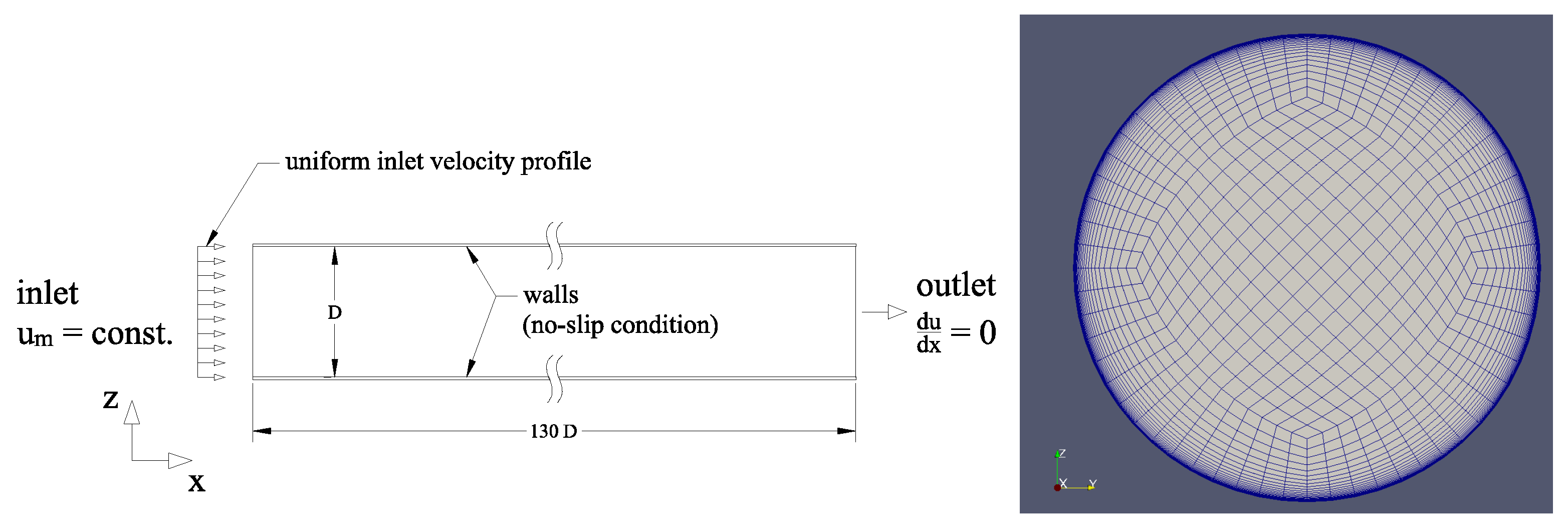
The presented method and its equations were solved using OpenFOAM (Open-source Field Operation And Manipulation) framework. OpenFOAM can be applied to simulate the condition occuring in HVAC systems [30]. It is open-source software with full access to the source code, thus facility the implementation of a subordinate models like the modified algebraic intermittency $k-\omega$ turbulence model [16]. The flow domain was a straight pipe with a length of $130D$. To perform the calculation a solver simpleFoam was used. All simulations have the same convergence criteria for velocity, pressure, turbulent kinetic energy, and specific dissipation rate, equals to ${10}^{-4}$.

3.1. Mesh

Computational domain was divided into a finite volume with the shape of hexahedra. The mesh was fully parametric with no automatic algorithm applied. To create a mesh suitable for OpenFOAM framework, a tool called blockMesh which is part of OpenFOAM was used. The frame of reference and mesh shape (No. 5 according to

Table 2. Results of ${\tau }_w/\rho$$\left[{\mathrm{m}}^2/{\mathrm{s}}^2\right]$ at the end of simulated duct for different meshes (modified $k-\omega$ model).

Mesh No.	Elements	$\mathbf{Re}=630$	$\mathbf{Re}=1680$	$\mathbf{Re}=2058$	$\mathbf{Re}=3108$
1	2,340,000	0.0002839	0.0007702	0.00096762	0.00294555
2	3,135,000	0.0002811	0.0007716	0.00102617	0.00221557
3	4,095,000	0.0002799	0.0007740	0.00131656	0.00257593
4	4,788,000	0.0002785	0.0007780	0.00143378	0.00283741
5	5,535,000	0.0002772	0.0007821	0.00145272	0.00288723
6	6,336,000	0.0002772	0.0007888	0.00147504	0.00292444

and

Table 3. Results of ${\tau }_w/\rho$$\left[{\mathrm{m}}^2/{\mathrm{s}}^2\right]$ at the end of simulated duct for different meshes ($k-\omega SST$ model).

Mesh No.	Elements	$\mathbf{Re}=630$	$\mathbf{Re}=1680$	$\mathbf{Re}=2058$	$\mathbf{Re}=3108$
1	2,340,000	0.0002871	0.0011365	0.00114578	unstable
2	3,135,000	0.0002869	0.0009390	0.00154990	0.00315847
3	4,095,000	0.0002869	0.0009146	0.00146410	0.00313742
4	4,788,000	0.0002873	0.0008736	0.00138051	0.00302111
5	5,535,000	0.0002873	0.0008679	0.00136535	0.00299605
6	6,336,000	0.0002874	0.0008523	0.00135157	0.00297665

) were presented in Figure 1.

Near the pipe wall, the size of elements was decreased. The $y^{+}$ value for a specific flow condition for the mesh No. 5 (according to Table 2 and Table 3) were presented in

Table 4. Mesh $y^{+}$ values.

Re	${\mathit{y}}^{+}$
630	0.016
1680	0.026
2058	0.036
3108	0.051

.

To calculate $y^{+}$ values, following equation was used:

$$y^{+}=\frac{y·\sqrt{{\tau }_w/\rho }}{\nu },$$

(13)

where ${\tau }_w$ (wall shear stress value) was determined according to the theoretical value of wall shear stress under steady-state conditions at the end of pipe:

$${\tau }_w=\mathsf{\Delta }p·\frac{D}{4·L}.$$

(14)

where $\mathsf{\Delta }p/L$ is a pressure loss according to the Darcy-Weisbach equation. The y length in Equation (13) was the height of the near wall element measured perpendicular to the wall face.

The mesh quality of mesh No. 5 was evaluated using OpenFOAM tool checkMesh. Maximum aspect ratio was equalled to 183.787. This value was determined by near wall elements. Maximum mesh skewness equals 0.5907 and the average mesh non-orthogonality was 4.4997. The maximum value of mesh non-orthogonality was 38.573. The mesh consist of 5,535,000 volume elements. To perform mesh independency study different meshes was generated. Result of simulation with these meshes was presented in Table 2 and Table 3. The value of steady wall shear stress was picked to show mesh independency [16]. The mesh No. 5 was choose because the relative difference between previous (No. 4) and next (No. 6) mesh according to steady wall shear stress value was less than $2\%$.

3.2. Boundary Conditions

Simulations were further compared with measurements performed for 4 different Reynolds numbers (Table 4). Reynolds number was defined as following:

$$\mathrm{Re}=\frac{u_m·D}{\nu }.$$

(15)

The inlet velocity $u_m$ was assumed as uniform at the inlet with a specific turbulence intensity $Tu$. The inlet turbulence intensity was estimated using correlation in CFD software like FLUENT:

$$Tu=0.16·R{e}^{-0.125}.$$

(16)

Turbulent intensity Formula (16) is sufficient for CFD simulations [31] and used for nonturbulent flow in tubes [32,33]. For the laminar flow, there is no need to define the turbulent intensity because the results are independent from $Tu$ values. Therefore, $Tu$ values are only calculated for the Reynolds number where transitional flow is suspected.

Turbulent kinetic energy k and specific dissipation rate $\omega$ for the inlet was calculated using following correlations [18]:

$$k=\frac{3}{2}{\left(u_m·Tu\right)}^2,\omega =\frac{\sqrt{k}}{l},$$

(17)

where l is turbulent length scale defined by $l=0.07·D$.

For the $k-\omega SST$ turbulence model, an additional boundary condition needs to be applied. The value of ${\mathrm{Re}}_{\theta t}$ at the inlet cross section is calculated using the correlations presented in [34] for $Tu>1.3$:

$${\mathrm{Re}}_{\theta t}=331.50·{[Tu-0.5658]}^{-0.671}·F\left({\lambda }_{\theta }\right),$$

(18)

where

$$F\left({\lambda }_{\theta }\right)=1;{\lambda }_{\theta }=0.$$

(19)

Estimated ${\mathrm{Re}}_{\theta t}$ and $Tu$ values for different Reynolds numbers ware presented in

Table 5. Flow parameters used in numerical simulations.

Re	Inlet $\mathit{Tu}$ [%]	${\mathbf{Re}}_{\mathit{\theta }\mathit{t}}$
1680	6.3	102.4
2058	6.2	104.3
3108	5.9	108.4

. Other boundary conditions were:

• inlet k and $\omega$ calculated using inlet turbulence intensity $Tu$;
• no slip velocity on walls;
• no wall function for k, $\omega$ and ${\nu }_t$ fields;
• constant pressure at the outlet;
• no velocity change at the outlet.

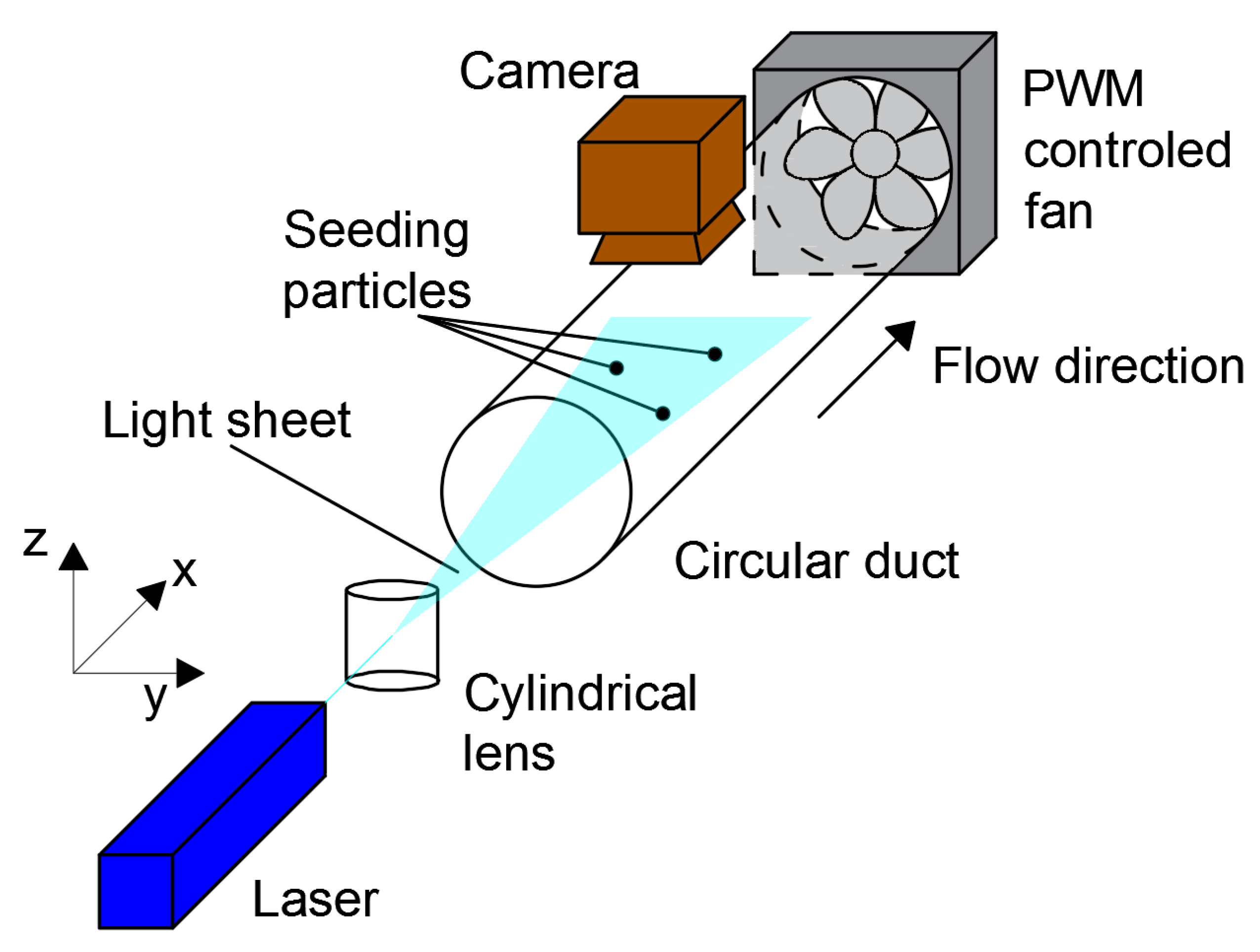
4. Experiment Setup

To perform model validation, a measurement using 2-dimensional PTV method was made. Authors decided to measure the velocity profile in one section ($x=32D$) of the pipe with different Reynolds numbers, because in this section can be observed the greatest change in velocity profile in pipe as pointed in [20,29]. Moreover in this section for Reynolds number $\mathrm{Re}=630$, the velocity profile was close to parabolic due to laminar flow. For greater Reynolds number, like $\mathrm{Re}=1680$ and $\mathrm{Re}=2058$, initial stadium of intermittent flow was observed. While for $\mathrm{Re}=3108$ starts of the turbulent flow can be seen. Therefore in a specific pipe cross-section ($x=32D$) with different Reynolds number, it can be observed different types of flow. Measurement setup was presented in Figure 2. In this setup, a laser with regulated pulse frequency and light intensity with a wavelength of 450 nm was used. To control PTV measurement process, the mean velocity was measured using CTA (Constant Temperature Anemometer). The anemometer probe was located in the duct near the end before fan, where the flow conditions are steady.

The CTA measurement was performed using BABUC/A device (manufacturer LSO Lastem s.r.l.) with hot wire anemometric probe BSV101 attached. Specification for BSV101 is given in

Table 6. CTA measurement parameters.

Range	0–45 m/s
Accuracy	0–0.5 m/s: $\pm 5$ cm/s
	0.5–1.5 m/s: $\pm 10$ cm/s
	>1.5 m/s: 4%
Response time	10 ms
Resolution	0.01 m/s
Sensing element	platinum wire $18\mathsf{\mu }$m

.

Temperature of the air in the experiment equals to 24.8 ${}^{\circ }$C and its dynamic viscosity was $1.739\times {10}^{-5}$ [Pa s].

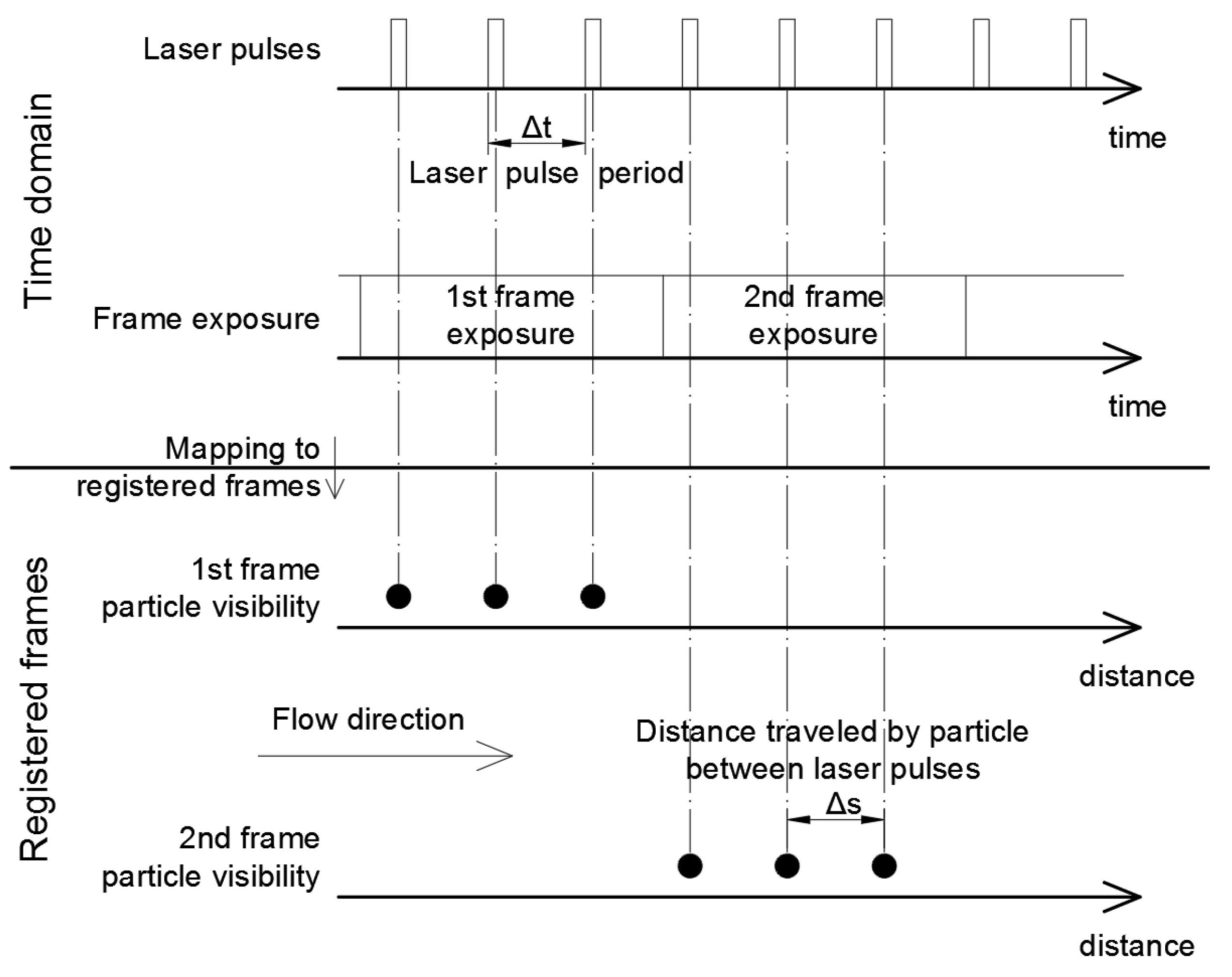
4.1. Measurement Method

General principle of the measurements was to obtain the velocity profile inside the tested pipe using PTV single-frame/multiple pulse method [35]. This was achieved by recording the moving particles inside the tested pipe and calculating the mentioned velocity profile based on the distance between given particle locations $\mathsf{\Delta }s$ along the pipe width and known frequency of laser pulse $1/\mathsf{\Delta }t$, where $\mathsf{\Delta }t$ is the laser pulse period. This method required low concentration of seeding particles and stable flow conditions during measurement.

4.2. Image Calibration

In order to provide valid values for measured $\mathsf{\Delta }s$ length, proper calibration using image scaling in length and height of the measured pipe was conducted. Image distortion due to light refraction through the pipe wall and other distortions was also taken into account. It was done by inserting the measure reference plane into the pipe fitted with laser sheet, and making the reference photography as seen in Figure 3 with the same parameters as in the image acquisition process with seeding particles. After obtaining the calibration image the reference plane was removed from the test duct.

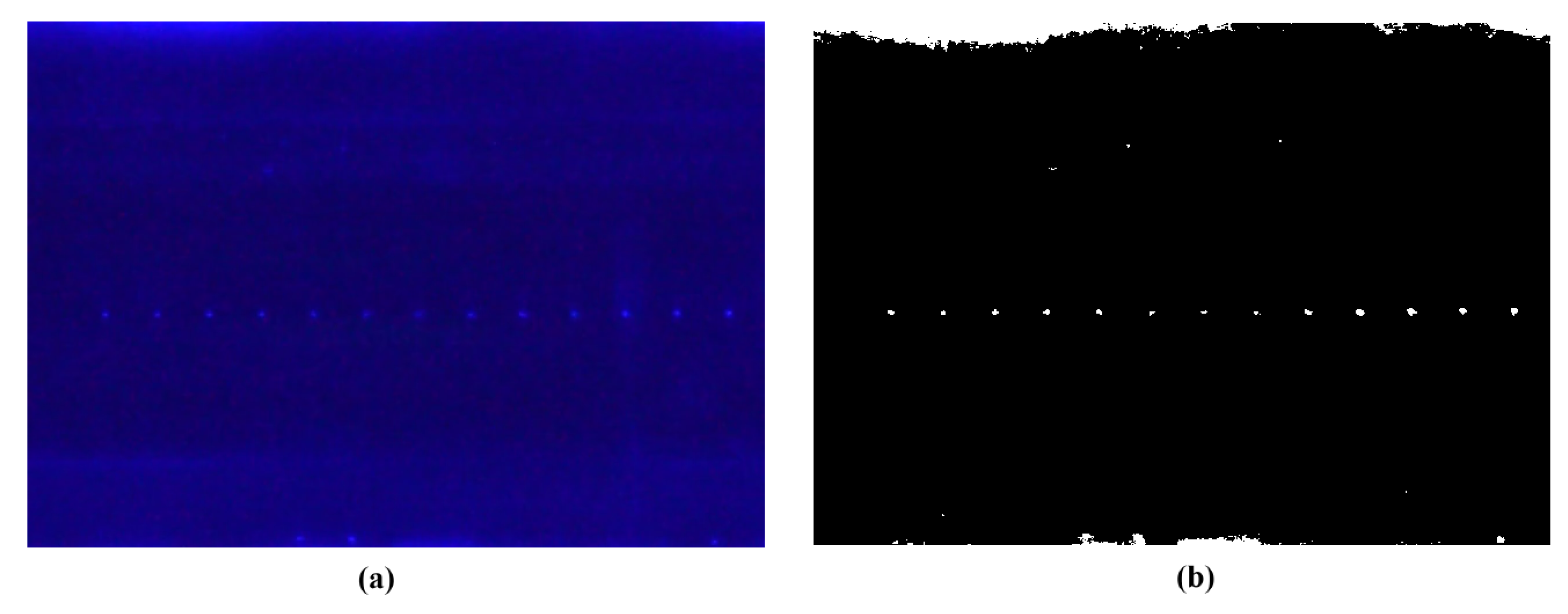
4.3. Image Processing

Image acquisition using PTV method was conducted by recording a movie with a duration of 60 s with 25 frames per second. Exposure time for each frame was equal to frame duration. Shutter setting was set to provide proper visibility of the tracked particles without the occurrence of motion blur of the recorded particles. Recording method was presented in Figure 4.

Value of 25 frames per second is dictated by the fact that in the measurement procedure $\mathsf{\Delta }s$ (which is the distance of a single particle travelled between the subsequent lasers pulses) is registered (as presented in Figure 4). Increase in frame exposure, thus a decrease in frame rate to 25 frames per second gives sufficient quantity in laser pulses—and distinct particle locations. Duration of image acquisition stems from the preliminary analysis of the convergence of coefficients A, B, C for the fitting curve given in Formula (20). The analysis of convergence of A, B, C consisted of 10 measurements of PTV for $\mathrm{Re}=3108$ for each given duration (5 s, 10 s, 15 s, ⋯ up to minimal duration meeting the requirements) for a fixed value of 25 frames per second. The requirements for this article were assumed to be as follows—average value of the coefficient is varying less than 0.5% two times in a row, the standard deviation value of the coefficient is less than 2% of the average coefficient value two times in a row. Minimal measurement duration is shown in

Table 7. CTA measurement parameters.

	Minimal Measurement Duration [s]
Coefficient of Equation (20)	A	B	C
Following average value of coefficient is varying less than 0.5% two times in a row	45	60	35
Following standard deviation value is for coefficient is less than 2% of average two times in a row	45	60	35

. The maximum value from the table below resulted in the measurement duration time. Convergence analysis was presented in Figure 5.

Method of recording seeding particle forces to ensure that the laser pulse frequency occurs at least twice during frame exposure. For practical purposes, during measurements the laser frequency was set to a constant value in range 100–400 Hz, so pulses occurred at least four times to avoid mistaking two different particles with a single one within two laser pulses. Exemplary seeding particle registration during measurement was presented in Figure 6.

4.4. Seeding Particle Type

Seeding particle diameter used in the measurements presented in this paper was approximately 10 $\mathsf{\mu }$m. The source of particles used in this measurement was the vapour of glycol triethylene. This size of the particle is good for the measurement type used in this study [36]. The device used for seeding particle was a fog generator Antari model F-80Z (with 0.7 kW heater) which heat up glycol triethylene to generate its vapor.

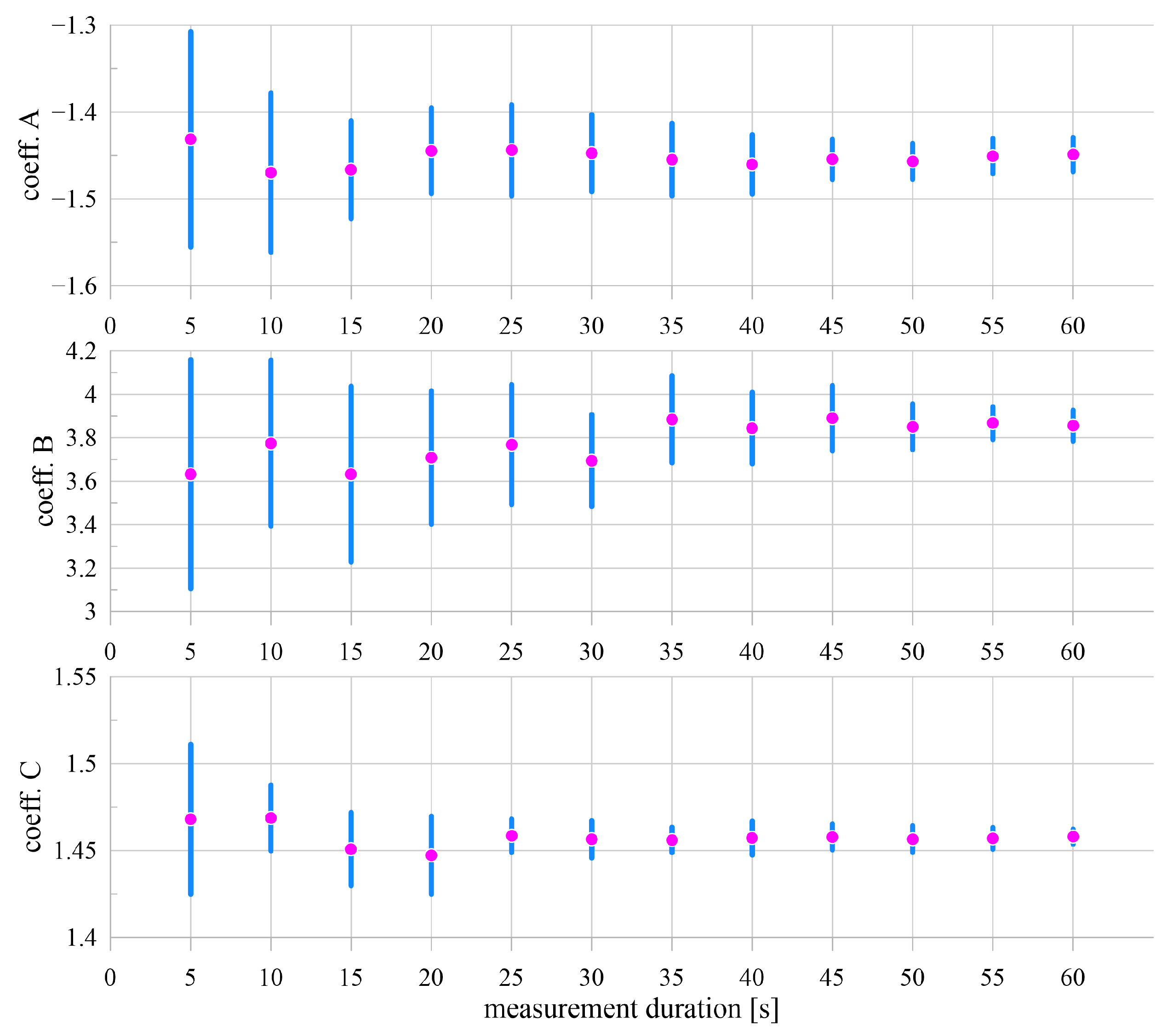
4.5. Image Analysis and Velocity Profile Calculation

Image analysis was done using MATLAB software. In general, PTV seeding particle localization using single frame/multiple pulse method is done by finding the next positions of seeding particles [35]. In this case, flow is stable and horizontal, method can be simplified as presented below. Threshold filter used in Matlab was built-in function imbinarize using adaptive threshold method on image (frame) converted to greyscale. Foreground polarity was set as bright to indicate that the foreground is brighter than background and sensitivity was set to manually (0.2–0.4).

After applying the threshold filter, the specific MATLAB script found the seeding particles first position starting from the left side of the analysed frame. The next step was to find the closest similar particle in the horizontal direction, which is in fact the same particle but in different position due to the subsequent laser pulse as described in Figure 4. Knowing the distance between these two particle locations, the next particle location is sought horizontally in the same direction using the previously calculated distance within 10% distance increase. This algorithm is applied for each seeding particle 1st position. After finding a group of particle positions (see Figure 6), the distances between the seeding particle positions were averaged. This method was done for each of the analysed frames (1500 frames in total). It is worth to underline that not every movie frame had a particle registered due to the low concentration of particles.

5. Results and Comparison

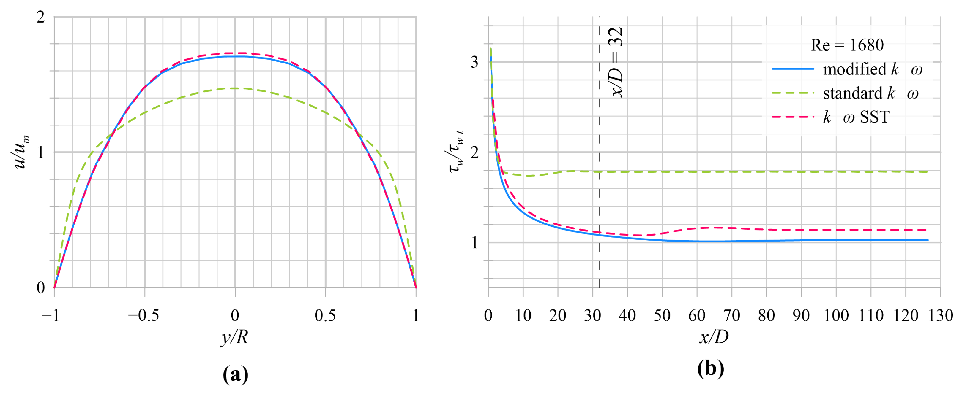
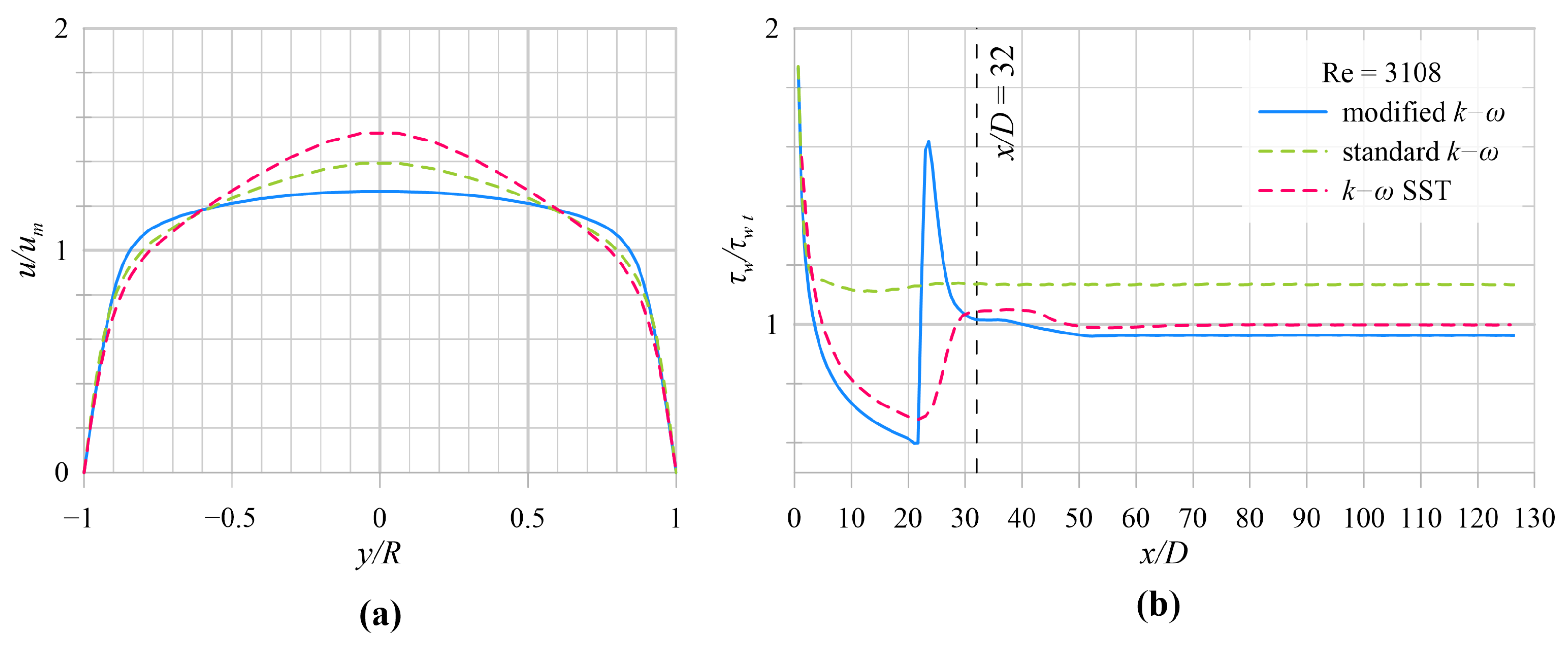
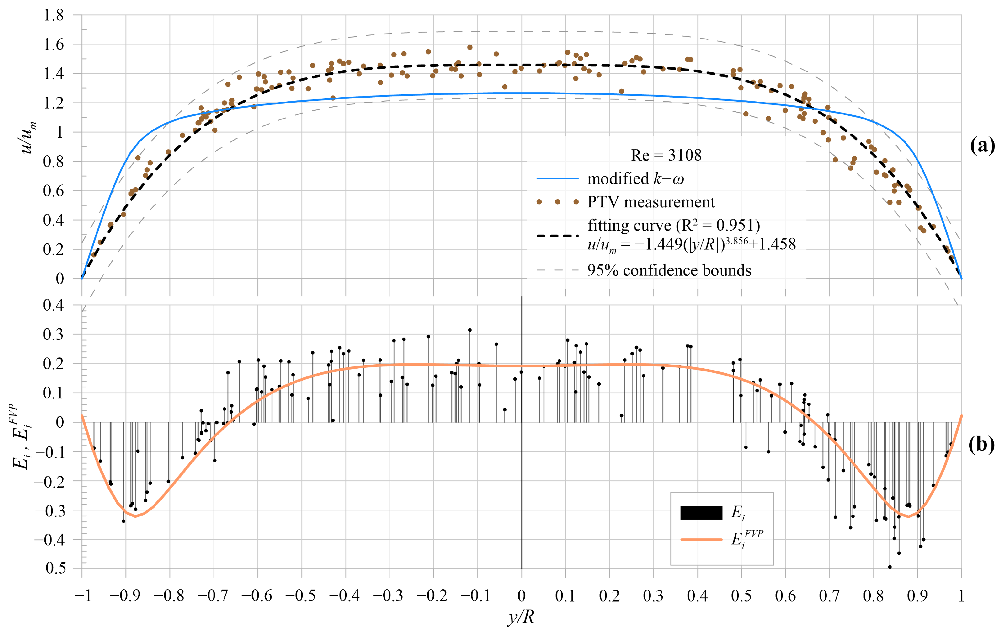
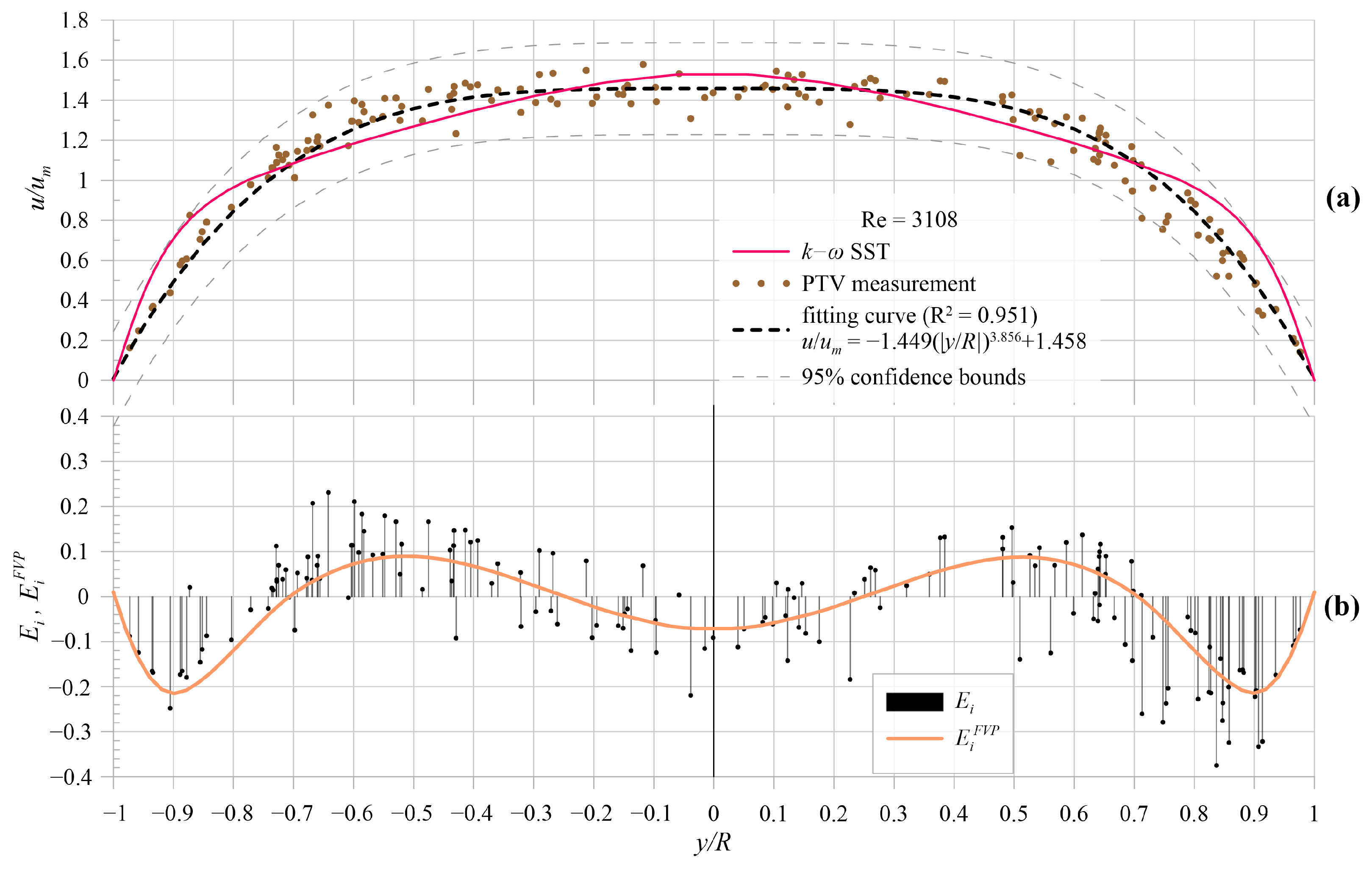
To validate the results obtained from model, a comparison with the experiment data was made. Three turbulence model results were presented: modified algebraic $k-\omega$ model, $k-\omega SST$ and standard $k-\omega$ by Wilcox [18,19]. First, to test the model usability steady-state fully-developed turbulent flow was modelled. Results of friction factor $\lambda$ were presented in Figure 7 with theoretical values of $\lambda$ for laminar $64/\mathrm{Re}$ and turbulent flow using Colebrook formula ${(1.8\times lo{g}_{10}\mathrm{Re}-1.51)}^{-2}$ [37].

As seen in Figure 7, standard $k-\omega$ is not suitable for transitional flow at all. However, with higher Reynolds number it gives the correct results. Better fitting is observed for the modified algebraic $k-\omega$ and $k-\omega SST$. Only significant differences but less than 10% are seen in the transitional flow near Reynolds number equals to 2000.

5.1. Model Results

The main purpose of numerical simulation was to obtain the velocity profiles in the specific cross-section of the analysed pipe. The section was located, as mentioned before, in $x=32D$ from the pipe inlet. In this section, for all four analysed values of the Reynolds number, different types of flow can be observed. In Figure 8, Figure 9, Figure 10 and Figure 11 the relative velocity profile (for cross-section $x=32D$) and relative wall shear stress are shown. Relative velocity is defined as the ratio of absolute velocity to the mean velocity of the flow ($u/u_m$). While the relative shear stress is obtained by dividing the absolute wall shear stress by shear stress calculated using theoretical friction factor values (${\tau }_w/{\tau }_{wt}\left(\lambda \right)$). The theoretical values of the shear stress was calculated using Equation (14).

Results obtained from the standard $k-\omega$ model show unphysical results—it was shown only for reference.

In Figure 8a, the velocity profiles for $k-\omega SST$ and modified $k-\omega$ are similar. Profiles do not reach theoretical values of 2 for laminar flow because in the analysed section the laminar flow is not fully developed. This can be observed from the shear stress curves in Figure 8b.

In Figure 9a, the velocity profiles start to show intermittent flow but only in the inlet section of pipe. Results from model $k-\omega SST$ and modified $k-\omega$ are similar as previously. Slight difference can be observed in the fully developed flow where $k-\omega SST$ shows increase of wall shear stress due to start of the transitional flow (Figure 9b). Modified $k-\omega$ model still show fully developed laminar flow without observed breakdown.

For Reynolds number equals to 2058, the differences between velocity profiles (Figure 10a) from the turbulence model $k-\omega SST$ and modified $k-\omega$ are significant. Laminar breakdown according to wall shear stress profiles (Figure 10b) occurs in section $x\approx 27D$. Extreme values of shear stress between the two models are different but the localisation of breakdown coincide. Shape of wall shear stress results from the modified $k-\omega$ model are sharpener due to the fact of the model formulation—it was also described in [20,26]. For $k-omegaSST$ shape of wall shear stress is compatible with [29]. In a specific cross-section $x=32D$, the velocity profiles near the wall have different velocity gradient which is correlated with the wall shear stress values.

The last analysis for $\mathrm{Re}=3108$ shows results similar to the previous Reynolds number. Velocity profile differs mainly in the centre of the pipe (Figure 11a), but near the wall the gradient of velocity is similar just like the wall shear stress values presented in Figure 11b. Laminar breakdown location for the modified $k-\omega$ and $k-\omega SST$ model is in the same location near $x\approx 21D$. Moreover the fully developed flows for these models occurs in the approximate region $x\approx 50D$.

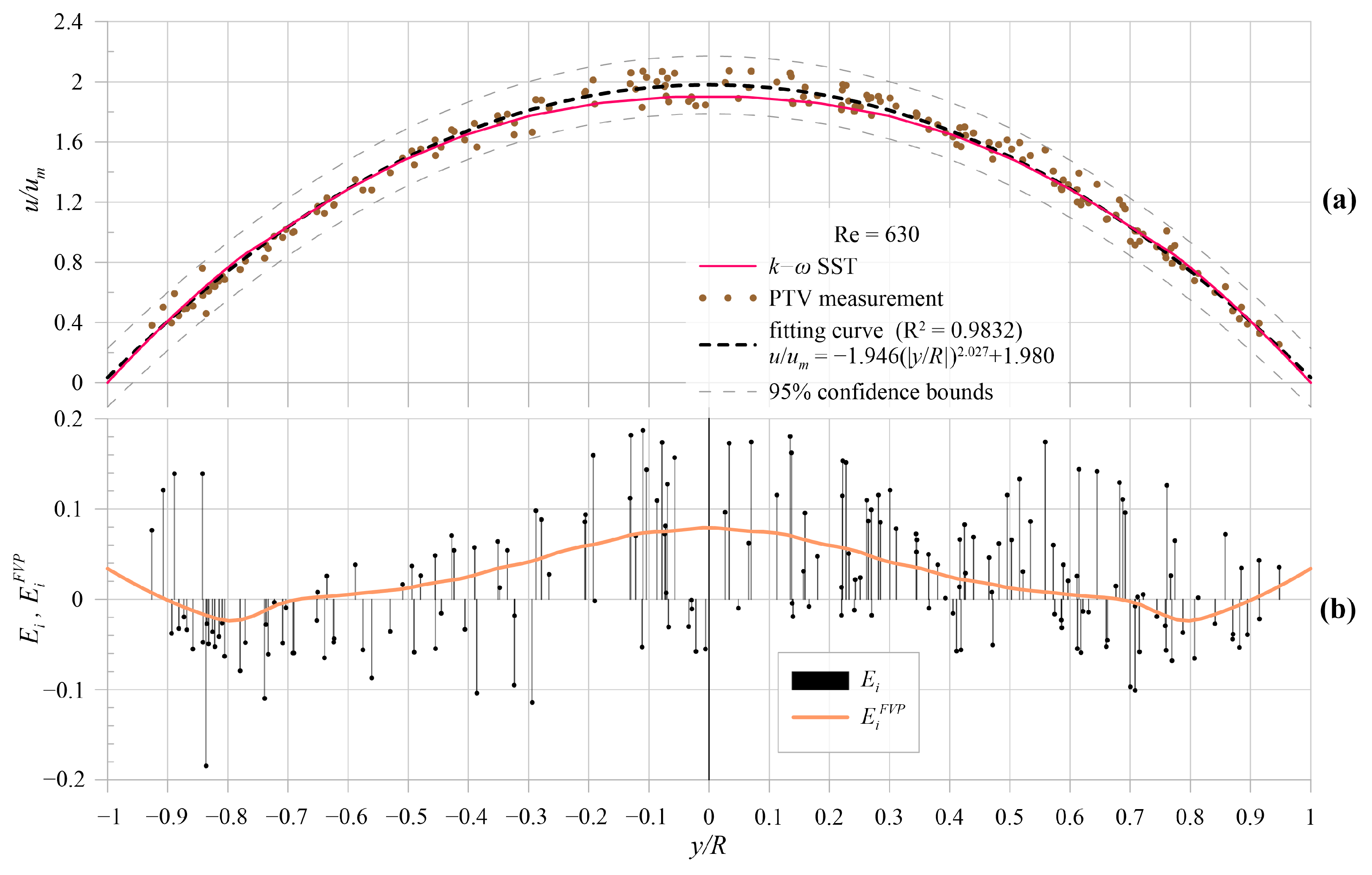
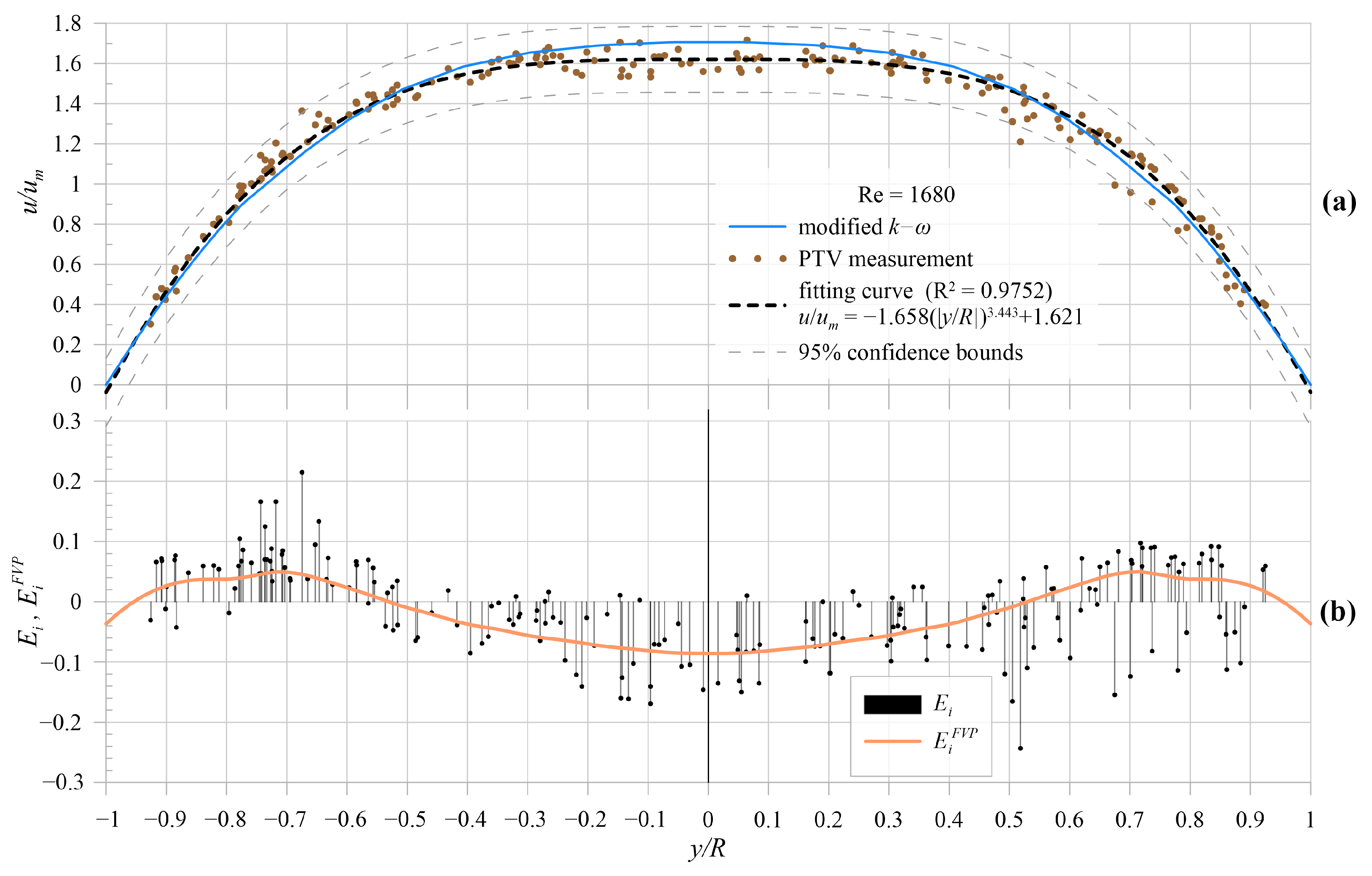
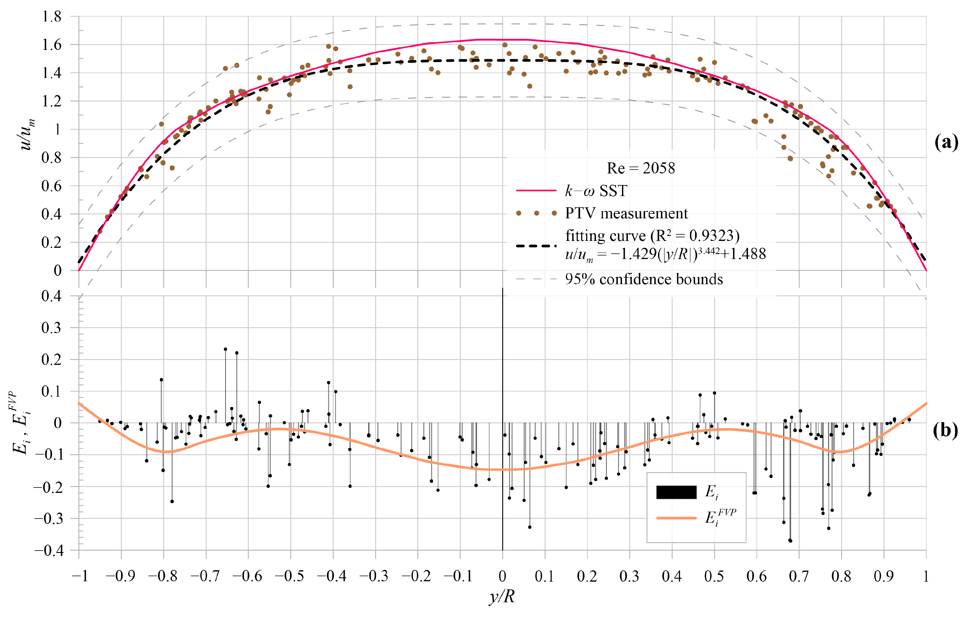
5.2. Experimental Model Validation

To validate the model results, a comparison with PTV measurement values was performed. All velocity profiles ware measured in the section at $x=32D$ of the pipe. Each measurement profile was fitted to a curve based on power law velocity profile [38]:

$$\frac{u}{u_m}{|}_{FVP}=A·{\left(\left|\frac{y}{R}\right|\right)}^B+C,$$

(20)

where A, B, and C are constants which were obtained during the regression analysis process.

For all Reynolds numbers, the validation of the modified $k-\omega$ model and $k-\omega SST$ was presented in Figure 12, Figure 13, Figure 14, Figure 15, Figure 16, Figure 17, Figure 18 and Figure 19. In each figure, a plot of error for each measurement point was presented. The error is defined as:

$$E_i=\frac{u_i{|}_{\mathrm{measurement}}}{u_m}-\frac{u_i{|}_{\mathrm{model}}}{u_m}.$$

(21)

Additionally, an error between the fitted velocity profile (FVP) and model results was presented:

$${E_i}^{FVP}=\frac{u}{u_m}{|}_{FVP}-\frac{{u|}_{\mathrm{model}}}{u_m}.$$

(22)

For $\mathrm{Re}=630$ in Figure 12, the measurement profile (a) with error (b) between measurement and the modified $k-\omega$ model was presented. This is a profile similar to the parabolic velocity distribution for laminar flow as mentioned before. In Figure 13 corresponding analysis for $k-\omega SST$ model was presented. It is worth mentioning that the profile of the standard $k-\omega$ model is not able to describe the laminar flow.

When laminar flows starts to breakdown in the inlet section of the flow for $\mathrm{Re}=1680$ velocity profile for both (modified $k-\omega$ and $k-\omega SST$) models, the velocity profile is flattened in the middle section of the pipe. This is shown in Figure 14a for modified $k-\omega$ and in Figure 15a for $k-\omega SST$. Errors are presented in (b) of corresponding figures.

For the transitional flow with $\mathrm{Re}=2058$, the modified $k-\omega$ model starts to underestimate the maximum velocity with a slight overestimate of velocity values near wall. This was shown in Figure 16a with error presentation in Figure 16b. The difference between the modified $k-\omega$ model and the measurement could be explained with the rapid increase of wall shear stress near the measured section as shown in Figure 10b. For $k-\omega SST$ analysis of the corresponding Reynolds number, results (a) with errors (b) are shown in Figure 17.

For the start of turbulent flow with $\mathrm{Re}=3108$, the modified $k-\omega$ model in the measured section of $x=32D$ shows an overestimation of velocity values in the middle section of the pipe while increasing the velocity in the near wall section. This was presented in Figure 18a,b where errors are shown. Velocity profile for the fully turbulent flow modelled and its comparison with measurement data was presented in [16]. Results for $k-omegaSST$ model are presented in Figure 19a,b.

To show the goodness of fitting for the model results with measurement, the root mean square error (RMSE) was calculated for each analysis using the following equation:

$$RMSE=\sqrt{\frac{{\sum }_{i=1}^N{E}_i^2}{N}},$$

(23)

where N is the number of measurements performed for each condition with the corresponding Reynolds number.

Value of RSME ware presented in

Table 8. Root Mean Square Error (RMSE) of compared results.

Re	Modified $\mathit{k}-\mathit{\omega }$	$\mathit{k}-\mathit{\omega }\mathbf{SST}$
630	0.072	0.078
1680	0.076	0.086
2058	0.151	0.119
3108	0.199	0.128

.

6. Discussion and Conclusions

To describe the laminar turbulent transition in the flowing fluid in HVAC circular channel, a modified algebraic model for by-pass transition was adapted. The model was tuned to satisfy the flow conditions specific for pipe flow. Numerical results were compared with the corresponding measurements of air flow through a circular channel using PTV method. Furthermore, the modified $k-\omega$ model was compared with widely used in these types of application model $k-\omega SST$. The main difference between modified $k-\omega$ and $k-\omega SST$ is the number of equations that solve turbulence. Modified $k-\omega$ consists of standard $k-$ and $\omega -$ equations with algebraic equations for the intermittency factor $\gamma$. Model $k-\omega SST$ consists of four partial differential equations for turbulent kinetic energy k, specific dissipation rate $\omega$, intermittency factor $\gamma$, and transition momentum thickness Reynolds number ${\mathrm{Re}}_{\theta t}$.

Measurement was performed for specific flow conditions for laminar, transitional, and turbulent flow. Modified $k-\omega$ shows good results in laminar and transitional flow. For turbulent flow the velocity profile of the model results show slightly higher error than other types of flow. It is due to the fact that the transition area modelled with algebraic model has a rapid change of wall shear stress and velocity profile. However, the location of transition corresponds to the correct values and the steady state fully developed turbulent flow also leads to correct wall shear stress values and correct velocity profile.

One of the advantages of the modified model is its calculation time. In comparison with $k-\omega SST$ simulation with the modified model needs approximately 50% less time to compute. Therefore, designing HVAC systems using the proposed model reduces the need for computing power.

The modified model can also be applied for other flow conditions that appear in HVAC systems - flow-through a pipe heat exchanger where the wall shear stress is crucial because of the dependence on the flow friction factor and heat transfer coefficient. However, the analysis of heat transfer coefficient with transitional flow needs further studies.

References

1. Shao, L.; Riffat, S. Accuracy of CFD for predicting pressure losses in HVAC duct fittings. Appl. Energy 1995, 51, 233–248. [Google Scholar] [CrossRef]
2. Zhong, W.; Zhang, T.; Tamura, T. CFD Simulation of Convective Heat Transfer on Vernacular Sustainable Architecture: Validation and Application of Methodology. Sustainability 2019, 11, 4231. [Google Scholar] [CrossRef] [Green Version]
3. Ren, C.; Cao, S.J. Development and application of linear ventilation and temperature models for indoor environmental prediction and HVAC systems control. Sustain. Cities Soc. 2019, 51, 101673. [Google Scholar] [CrossRef]
4. Pichurov, G.; Stankov, P.; Markov, D. Hvac control based on CFD analysis of room airflow. IFAC Proc. Vol. 2006, 39, 213–218. [Google Scholar] [CrossRef]
5. Tian, W.; Han, X.; Zuo, W.; Wang, Q.; Fu, Y.; Jin, M. An optimization platform based on coupled indoor environment and HVAC simulation and its application in optimal thermostat placement. Energy Build. 2019, 199, 342–351. [Google Scholar] [CrossRef]
6. Adegbenro, A.; Short, M.; Angione, C. An Integrated Approach to Adaptive Control and Supervisory Optimisation of HVAC Control Systems for Demand Response Applications. Energies 2021, 14, 2078. [Google Scholar] [CrossRef]
7. Taler, D. Determining velocity and friction factor for turbulent flow in smooth tubes. Int. J. Therm. Sci. 2016, 105, 109–122. [Google Scholar] [CrossRef]
8. Abraham, J.; Sparrow, E.; Tong, J. Heat transfer in all pipe flow regimes: Laminar, transitional/intermittent, and turbulent. Int. J. Heat Mass Transf. 2009, 52, 557–563. [Google Scholar] [CrossRef]
9. Rup, K.; Duda, P.; Danys, L. Determination of heat transfer coefficients on the surfaces of plastic tubes. Heat Mass Transf. 2002, 39, 89–95. [Google Scholar] [CrossRef]
10. Fernando, N.; Narayana, M. Limiting value of Reynolds Averaged Simulation in numerical prediction of flow over NACA4415 airfoil. In Proceedings of the 2016 Moratuwa Engineering Research Conference (MERCon), Moratuwa, Sri Lanka, 5–6 April 2016. [Google Scholar] [CrossRef]
11. Boiko, A.V.; Demyanko, K.V.; Inozemtsev, A.A.; Kirilovskiy, S.V.; Nechepurenko, Y.M.; Paduchev, A.P.; Poplavskaya, T.V. Determination of the laminar-turbulent transition location in numerical simulations of subsonic and transonic flows past a flat plate. Thermophys. Aeromech. 2019, 26, 629–637. [Google Scholar] [CrossRef]
12. Kirilovskiy, S.V.; Boiko, A.V.; Demyanko, K.V.; Ivanov, A.V.; Nechepurenko, Y.M.; Poplavskaya, T.V. Numerical simulation of the laminar-turbulent transition on a swept wing in a subsonic flow. J. Phys. Conf. Ser. 2019, 1359, 012070. [Google Scholar] [CrossRef]
13. Abdollahzadeh, M.; Esmaeilpour, M.; Vizinho, R.; Younesi, A.; Pàscoa, J. Assessment of RANS turbulence models for numerical study of laminar-turbulent transition in convection heat transfer. Int. J. Heat Mass Transf. 2017, 115, 1288–1308. [Google Scholar] [CrossRef]
14. Vizinho, R.; Páscoa, J.; Silvestre, M. Turbulent transition modeling through mechanical considerations. Appl. Math. Comput. 2015, 269, 308–325. [Google Scholar] [CrossRef]
15. Kubacki, S.; Dick, E. An algebraic model for bypass transition in turbomachinery boundary layer flows. Int. J. Heat Fluid Flow 2016, 58, 68–83. [Google Scholar] [CrossRef]
16. Nering, K.; Rup, K. An improved algebraic model for bypass transition for calculation of transitional flow in parallel-plate channel. Int. J. Therm. Sci. 2019, 135, 471–477. [Google Scholar] [CrossRef]
17. Bernardos, L.; Richez, F.; Gleize, V.; Gerolymos, G.A. Algebraic Nonlocal Transition Modeling of Laminar Separation Bubbles Using k-ω Turbulence Models. AIAA J. 2019, 57, 553–565. [Google Scholar] [CrossRef]
18. Wilcox, D. Turbulence Modeling for CFD; DCW Industries: La Canada, CA, USA, 2006. [Google Scholar]
19. Wilcox, D.C. Formulation of the k-w Turbulence Model Revisited. AIAA J. 2008, 46, 2823–2838. [Google Scholar] [CrossRef] [Green Version]
20. Nering, K.; Rup, K. Modified algebraic model of laminar-turbulent transition for internal flows. Int. J. Numer. Methods Heat Fluid Flow 2019, 30, 1743–1753. [Google Scholar] [CrossRef]
21. You, H.; Tinoco, R.O. Quantifying the Response of Grass Carp Larvae to Acoustic Stimuli Using Particle-Tracking Velocimetry. Water 2021, 13, 603. [Google Scholar] [CrossRef]
22. Özdemir, O.Ç.; Conahan, J.M.; Müftü, S. Particle Velocimetry, CFD, and the Role of Particle Sphericity in Cold Spray. Coatings 2020, 10, 1254. [Google Scholar] [CrossRef]
23. Wang, R.; Duan, R.; Jia, H. Experimental Validation of Falling Liquid Film Models: Velocity Assumption and Velocity Field Comparison. Polymers 2021, 13, 1205. [Google Scholar] [CrossRef]
24. Yang, T.; Liu, Z.; Chen, Y.; Yu, Y. Real-Time, Inexpensive, and Portable Measurement of Water Surface Velocity through Smartphone. Water 2020, 12, 3358. [Google Scholar] [CrossRef]
25. Ma, J.; Niu, X.; Liu, X.; Wang, Y.; Wen, T.; Zhang, J. Thermal Infrared Imagery Integrated with Terrestrial Laser Scanning and Particle Tracking Velocimetry for Characterization of Landslide Model Failure. Sensors 2019, 20, 219. [Google Scholar] [CrossRef] [PubMed] [Green Version]
26. Nering, K.; Rup, K. An improved algebraic model for by-pass transition for calculation of transitional flow in pipe and parallel-plate channels. Therm. Sci. 2019, 23, 1123–1131. [Google Scholar] [CrossRef] [Green Version]
27. Menter, F.R.; Langtry, R.B.; Likki, S.R.; Suzen, Y.B.; Huang, P.G.; Völker, S. A Correlation-Based Transition Model Using Local Variables: Part I — Model Formulation. In Proceedings of the ASME Turbo Expo 2004: Power for Land, Sea, and Air, Vienna, Austria, 14–17 June 2004. [Google Scholar] [CrossRef] [Green Version]
28. Langtry, R.B.; Menter, F.R.; Likki, S.R.; Suzen, Y.B.; Huang, P.G.; Völker, S. A Correlation-Based Transition Model Using Local Variables—Part II: Test Cases and Industrial Applications. J. Turbomach. 2004, 128, 423–434. [Google Scholar] [CrossRef]
29. Abraham, J.P.; Sparrow, E.M.; Tong, J.C.K. Breakdown of Laminar Pipe Flow into Transitional Intermittency and Subsequent Attainment of Fully Developed Intermittent or Turbulent Flow. Numer. Heat Transf. Part B Fundam. 2008, 54, 103–115. [Google Scholar] [CrossRef]
30. Rabani, M.; Madessa, H.B.; Nord, N. Building Retrofitting through Coupling of Building Energy Simulation-Optimization Tool with CFD and Daylight Programs. Energies 2021, 14, 2180. [Google Scholar] [CrossRef]
31. Russo, F.; Basse, N.T. Scaling of turbulence intensity for low-speed flow in smooth pipes. Flow Meas. Instrum. 2016, 52, 101–114. [Google Scholar] [CrossRef]
32. Badar, A.; Buchholz, R.; Lou, Y.; Ziegler, F. CFD based analysis of flow distribution in a coaxial vacuum tube solar collector with laminar flow conditions. Int. J. Energy Environ. Eng. 2012, 3, 24. [Google Scholar] [CrossRef] [Green Version]
33. García-Guendulain, J.; Riesco-Avila, J.; Elizalde-Blancas, F.; Belman-Flores, J.; Serrano-Arellano, J. Numerical Study on the Effect of Distribution Plates in the Manifolds on the Flow Distribution and Thermal Performance of a Flat Plate Solar Collector. Energies 2018, 11, 1077. [Google Scholar] [CrossRef] [Green Version]
34. Langtry, R. Extending the Gamma-Rethetat Correlation based Transition Model for Crossflow Effects (Invited). In Proceedings of the 45th AIAA Fluid Dynamics Conference, Dallas, TX, USA, 22–26 June 2015. [Google Scholar] [CrossRef]
35. Cierpka, C.; Lütke, B.; Kähler, C.J. Higher order multi-frame particle tracking velocimetry. Exp. Fluids 2013, 54. [Google Scholar] [CrossRef] [Green Version]
36. Hadad, T.; Gurka, R. Effects of particle size, concentration and surface coating on turbulent flow properties obtained using PIV/PTV. Exp. Therm. Fluid Sci. 2013, 45, 203–212. [Google Scholar] [CrossRef]
37. Colebrook, C.F. Turbulent flow in pipes, with particular reference to the transition region between the smooth and rough pipe laws. J. Inst. Civ. Eng. 1939, 11, 133–156. [Google Scholar] [CrossRef]
38. Afzal, N.; Seena, A.; Bushra, A. Power Law Velocity Profile in Fully Developed Turbulent Pipe and Channel Flows. J. Hydraul. Eng. 2007, 133, 1080–1086. [Google Scholar] [CrossRef]
Figure 1. Geometrical model with boundary conditions.
Energies 14 03975 g001
Figure 2. Measurement setup.
Energies 14 03975 g002
Figure 3. Reference calibration image in pipe middle cross-section.
Energies 14 03975 g003
Figure 4. Principle of image processing during the measurement.
Energies 14 03975 g004
Figure 5. Convergence analysis of A, B, C coefficient (from Equation (20)) using mean value from 10 measurements (dots) with standard deviation (vertical lines) against measurement duration time.
Energies 14 03975 g005
Figure 6. Seeding particle recorded during the measurement process (a) raw frame image, and (b) frame image with applied threshold filter.
Energies 14 03975 g006
Figure 7. Variation of the fully developed friction factor, λ , for pipe flow.
Energies 14 03975 g007
Figure 8. Modelled velocity profile for x = 32 D (a) and relative wall shear stress in pipe (b) for Re = 630 .
Energies 14 03975 g008
Figure 9. Modelled velocity profile for x = 32 D (a) and relative wall shear stress in pipe (b) for Re = 1680 .
Energies 14 03975 g009
Figure 10. Modelled velocity profile for x = 32 D (a) and relative wall shear stress in pipe (b) for Re = 2058 .
Energies 14 03975 g010
Figure 11. Modelled velocity profile for x = 32 D (a) and relative wall shear stress in pipe (b) for Re = 3108 .
Energies 14 03975 g011
Figure 12. Comparison between PTV measurement and simulation with modified k ω model for Re = 630 (a) with error values (b).
Energies 14 03975 g012
Figure 13. Comparison between PTV measurement and simulation with k ω S S T model for Re = 630 (a) with error values (b).
Energies 14 03975 g013
Figure 14. Comparison between PTV measurements and simulations with modified k ω model for Re = 1680 (a) with error values (b).
Energies 14 03975 g014
Figure 15. Comparison between PTV measurements and simulations with k ω S S T model for Re = 1680 (a) with error values (b).
Energies 14 03975 g015
Figure 16. Comparison between PTV measurements and simulations with modified k ω model for Re = 2058 (a) with error values (b).
Energies 14 03975 g016
Figure 17. Comparison between PTV measurements and simulations with k ω S S T model for Re = 2058 (a) with error values (b).
Energies 14 03975 g017
Figure 18. Comparison between PTV measurements and simulations with modified k ω model for Re = 3108 (a) with error values (b).
Energies 14 03975 g018
Figure 19. Comparison between PTV measurements and simulations with k ω S S T model for Re = 3108 (a) with error values (b).
Energies 14 03975 g019