Article

On the Optimization of Electrical Water Heaters: Modelling Simulations and Experimentation

1
Energy and Thermo-Fluid Group, Lebanese International University LIU, Bekaa 1803, Lebanon
2
Energy and Thermo-Fluid Group, International University of Beirut BIU, Beirut 146404, Lebanon
3
Faculty of Technology, Lebanese University, Saida 1600, Lebanon
*
Author to whom correspondence should be addressed.
Energies 2021, 14(13), 3912; https://doi.org/10.3390/en14133912
Submission received: 20 May 2021 / Revised: 16 June 2021 / Accepted: 25 June 2021 / Published: 29 June 2021

Abstract

:
In the context of a world energy crisis, the only solution to control the situation is in the management of energy. One of the most important management keys is the optimization of electrical components. This article presents a complete numerical and experimental study aiming for the optimization of electrical water heaters for household use. The optimization conceives the minimization of energy consumption simultaneously with the minimization of time to heat water. Firstly, a thermal model well adapted for the case of heaters is constructed and validated experimentally and then a parametric study is conducted covering all the input power, the volume and the external area of the heater. Results are promising, showing significant energy savings are possible with an optimum setting of these parameters, thus presenting a firm tool for the optimization of heaters.

1. Introduction

Due to the aggravation of an energy crisis, Scientists recommend exploiting renewable sources of energy [1,2,3] and to simultaneously manage the energy consumption as a last step to reduce the severity of this problem [4,5,6,7]. The energy management field is under continuous development nowadays due to the diversity and complexity of components involved in modern thermal systems. Particularly, household water heating is one of the most energy consuming applications, especially in countries with cold winter. It is commonly known that electrical resistance is the worst means to heat water, particularly in terms of wasting energy. Scientists recognize that replacing electrical heaters with more efficient systems such as heat pumps can recover heat even from wastewater [8]. However, electrical water heaters are still being manufactured in large quantities all around the world and face almost no purchasing resistance. Reasons behind the persistent presence of this device in the market are numerous, but the ultimate reason is the practicality of installing and using the device. This paper presents a parametric study on electrical water heaters aiming to optimize the design in order to reduce supplementary energy losses and potentially increase user comfort.
Before starting discussions about specific details of electrical water heaters, a brief historical review on alternative solutions is necessary. Many studies have been carried out on heat recovery systems or waste burning systems in order to reduce the use of electricity [9,10,11,12,13]. Other alternative systems are based on solar energy which is completely a renewable energy. Nowadays, commercial solar heaters are used all around the world [14,15,16]. However, flame-based systems are relatively complicated systems, while solar heaters have a difficult requirement which is available space in a solar-exposed location. Moreover, their efficiency is influenced by several parameters, such as shadings and weather conditions, in addition to their passivity during nighttime [17]. Therefore, these heaters are usually equipped with an electric resistance to heat the water when the solar irradiance is insufficient, thus giving a supplementary reason for the use of electricity.
A recent survey was conducted on several groups of people in different countries with the purpose of investigating how people interact with the energy crisis. One of the principal objectives was to quantify the awareness and energy-saving measures concerning the use of electric water heaters. In USA and South Africa, the majority of participants responded with curtailment actions, such as taking showers with minimum water, while in Japan, consumers proposed energy-saving actions, such as installing solar water heaters [18].
More specific studies were carried out on electrical heaters themselves in order to check the possibility of enhancing their performance. For instance, to rate the performance of dwelling electric water heaters, an experimental program was carried out in 2016 testing ten boilers with different capacities and different potencies [19]. The time needed to heat the whole quantity of water in each tank was shown to be in direct relation with both the tank’s volume and electrical power. Other works focus on system monitoring and underline its benefits in terms of energy management. In 2013, Booysen et al. showed that for a typical hot water consumption of 75 L per day, a savings of 1.4 kWh can be obtained each day just by turning monitoring on [20]. In 2002, Sateikis [21] studied the effects of temperature distribution inside the tank on energetic efficiency. He presented an experiment on vertical boilers with diameter dimensions of 0.3 and 0.9 m and heights of 1.6 and 2 m in function to determine the capacity of thermal energy preserved inside the boilers.
Examining the literature, although many technologies can replace classical water heaters equipped with electrical resistances, these heaters are still needed worldwide. These types of heaters are energy consuming and their energy consumption is highly dependent on many important parameters such as the input power, the volume and the shape and area of the heater tank. Minimal studies investigate the influence of the relevant parameters in a parametric way and optimize the heater operation accordingly. In this context, the present manuscript presents a parametric study of electrical water heating using validated simplified modular thermal modeling.
This study represents an energetic investigation of some parameters of residential water heaters and how they affect the efficiency of these heaters. To proceed, thermal modeling of a typical water heater is first presented, as well as a relevant experimental method for determining the overall heat transfer coefficient. Then a parametric study is presented showing the effects of the tank’s volume, power and shape on the heater’s performance. This work presents an important tool for the optimization of water heaters for better energy management in buildings.
Concerning energy management, the literature is replete with algorithms and tools for simulation and optimization in regard to efficient energy management in building heating systems [22]. An investigation on the specific issue of advanced control system design for energy efficient buildings was presented by Ma et al. in 2012 [23].
In 2016, O’Dwyer et al. proposed a novel spatio-temporal filtering technique for disturbance estimation and employed metaheuristic search methods to permit derivation of models through data where typical disturbances are present [24]. Due to this disturbance estimation, low-order models suited in an optimization-based Model Predictive Control MPC strategy could be derived. The modelling concepts were set with real building data and a potential MPC formulation was assessed.
One year later, O’Dwyer et al. presented an MPC-based building heating strategy where energy savings and thermal comfort were optimized in a prioritized manner [25].
Having balanced weights in the objective function is not required, making the strategy design simpler. Moreover, high-order linear optimization is separated from low-order, non-linear optimization by dividing the problem into supply and demand problems.
In the same year (2017), Fiorentini et al. presented a hybrid MPC strategy, providing the development and experimental testing. The strategy aimed to control a heating, ventilating and air conditioning (HVAC) system which was solar assisted [26]. It aimed to optimize the utilization schedule of thermal energy resources to maintain comfort conditions by presenting a comprehensive technique for residential building thermal management.
In 2019, Kuboth et al. [27] investigated an economic MPC of residential energy systems of a complex nature, electrically coupled with the public grid. The system is composed of a building model, thermal energy storage, an air-to-water heat pump, a photovoltaic power generation and a battery energy storage system. The generated power supplies electrical loads, space heating and water heating. The energy system is managed by MPC through non-linear global optimization, in which system dynamics are reflected by a time-varying state space model. As a result of the system being highly complex, two algorithms for distributed MPC are obtained.
As shown above, MPC techniques for building energy system controls have been extensively investigated and their advantages are well demonstrated. A pivotal necessity for successful realization of these techniques is that the control strategies are formulated such that they are suitable for a variety of buildings with little commissioning effort.
The objective of the current manuscript examines optimization of building energy operation, particularly heating systems, but differs from the studies presented above in the following way:
  • Most of the studies consider complex systems of building operation, while the present paper is focused only on water tank heating systems and their thermal behavior.
  • Most of the studies develop very complex predictive optimization techniques that simultaneously treat the effect of several parameters to sort out optimized configurations, while the present manuscript constitutes simplified thermal modeling and its associated numerical tool which permits it to easily perform parametric studies of effects separately and jointly (as detailed in the manuscript).
  • Most of the studies concentrate on the mathematical side of the optimization, while the present paper concentrates on the thermal-energy side towards optimization.
  • Finally, the present work constitutes a solid basis for the future development of new optimization techniques by using the simulation tool presented as part of an overall optimization algorithm, especially when it comes to the water heating and the time of power utilization.
The originality of this work resides in the following points:
  • It proposes an appropriate simplified and modular thermal modeling of electrical water heater that facilitates performing parametric studies with low computational time.
  • The study presents a significant material in which the performance of electrical water heaters is investigated by undergoing a viable thermal modeling and performing parametric analysis.
  • It provides useful modeling and parametric analysis for the electrical water heater community. This benefit is achieved when the conducted thermal model is utilized in investigations aimed at energy management of the operation of electrical water heaters. It also facilitates studying the effects on system performance of a large range of parameters, especially when investigating the feasibility of new concepts or configurations.

2. Thermal Modeling

2.1. Energy Balance and Governing Equations

An electrical water heater is usually sized by its electrical power P and its tank’s volume V. The energy equation applied to the water inside the tank can be written as follows [12]:
E ˙ i n E ˙ o u t + E ˙ g = E ˙ s t
where E ˙ i n is the rate of the energy input transfer from the surrounding to the system (volume of water), E ˙ o u t is the rate of the energy transfer out from the system to the surrounding, E ˙ g is the rate of energy generated within the system (electric power P), and E ˙ s t is the rate of the change of energy stored within the system.
There is no energy input to the system from the surrounding. The output energy from the system to the surrounding is determined by convection and is expressed as:
E ˙ o u t = U A T w T a
where U is the overall heat transfer coefficient, A is the contact surface area, T w is water temperature through the control volume, and T a is the ambient air temperature.
The rate of energy stored within the control volume responsible for increasing the water temperature to a specified value during a specific period of time is expressed as:
E ˙ s t = ρ C p V T t
where ρ is the water density (997 kg/m3), C p the water specific heat (4178 J/Kg.K), V is the volume of the tank, T is the water temperature, and t is the time.
Applying Equation (1) to the control volume of Figure 1, this requirement takes the form:
E ˙ o u t + E ˙ g = E ˙ s t
By combining this equation with Equations (2) and (3), we get:
U A T w T a + P = ρ C p V T t
Introducing a temperature difference θ = T T a , where d θ / d t = d T / d t , Equation (5) reduces to a linear, first-order, nonhomogeneous differential equation of the form:
d θ d t + a θ + b = 0
where   a = U A / ρ C p V and b = P / ρ C p V . Although Equation (6) may be solved by summing its homogenous and particular solutions, an alternative approach is to eliminate the non-homogeneity by introducing the transformation:
θ = θ b a
Recognizing that d θ / d t = d θ / d t , Equation (7) may be substituted into (6) to yield:
d θ d t + a θ = 0
Separating variables and integrating with respect to time from 0 to t ( θ i to θ ) leads to:
θ θ i   = exp a t
Substituting for θ i and θ :
T T a b / a T w i T a b / a = exp a t
where T w i is the water initial temperature.
Hence:
T t = T w , i exp U A t ρ V C p + T a + P U A 1 exp U A t ρ V C p

2.2. Experimental Determination of the Overall Heat Transfer Coefficient

One of the important parameters of Equation (11) is the overall heat transfer coefficient (U). The overall heat transfer coefficient is the absolute heat transfer coefficient among the inside and the outside of the system. This coefficient takes into consideration convection between the external surface of the heater tank with ambient air, conductions in the tank material and insulation, and convection between the internal surface of the heater tank and water. Therefore, the accuracy of determination of the U is highly dependent on the determination of the convective and conductive thermal resistances, which is usually performed using correlations that do not have high precision. In this context, an experimental method for determination of U is suggested in this section. This method is based on experimental data and permits to obtain U with high accuracy. This coefficient obtained experimentally will be then incorporated in the thermal modeling to increase its accuracy.
Temperature measurements were achieved on a cylindrical water tank of 35 L, vertical with a height of 1 m and equipped with a 1200 W electrical resistance. The experiment consists of measuring the water temperature at the top of the tank every 2 min starting from activating the electrical resistance until the measured temperature reaches 80 °C. The initial temperature of water (Twi) and the ambient temperature (Ta) were both 20 °C. Equation (11) was used where the parameters (A, V, P, Ta, Twi) were replaced by the real values used in the experiment.
To proceed with the determination of U, as a first step U is considered known. In this case, the water temperature variation as per the modeling is:
T m o d e l i n g t = T w , i , e c p exp U A e x p t ρ V e x p C p + T a , e x p + P e x p U A e x p 1 exp U A e x p t ρ V e x p C p
where the subscript exp refers to experimental data.
Then, the value of U will be adjusted in an iterative way so that the magnitude of the error vector is minimized:
E = T e x p t i T m o d e l i n g
The registered overall heat transfer coefficient was 8.5 W/m2·K.

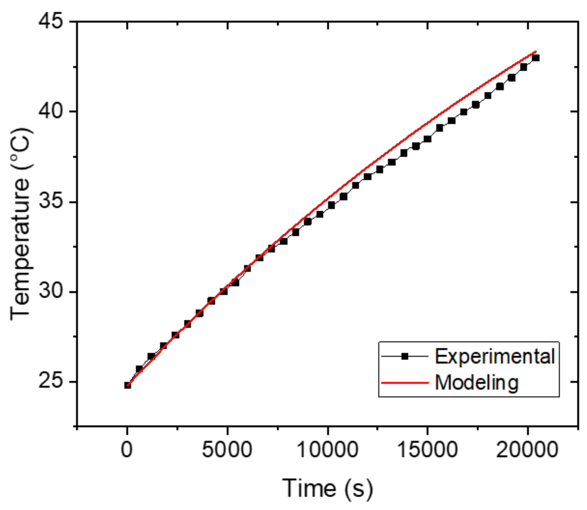
2.3. Experimental Validation

In this section, water temperature variation obtained with the modeling presented in Section 2.1 and Section 2.2 is compared to experimental variation using the same parameters. To proceed, temperature measurements were achieved on a cylindrical water tank of 100 L, vertical with a height of 1.05 m and diameter of 350 mm and equipped with a 500 W electrical resistance. The experiment consists of measuring the water temperature at the top of the tank every 5 min starting from activating the electrical resistance. The initial temperature of water (Twi) and the ambient temperature (Ta) were both 24.8 °C.
Figure 1 shows the water temperature variations obtained with the modeling and the experiment.
As shown in Figure 1, numerical values are close to their experimental counterparts. The relative error of temperature prediction with the modeling with respect to the experimental measurement is calculated throughout the entire period of experiment. A maximum relative error of 2.32% and an average relative error of 1.17% were obtained. Therefore, the modeling has sufficient accuracy to be used for temperature prediction, especially when it comes to performing parametric and case studies.

3. Parametric Study

Optimization of electrical water heating in terms of design can be defined by three main objectives: (1) minimizing the time of heating for more productivity, (2) minimizing the required power and (3) reducing losses. This optimization can be done by varying one of the parameters present in the Equation (11). This variation is associated with a change in the thermal behavior inside and across the boundaries of the heater tank, which was considered as a vertical cylindrical in all cases. Three parameters were studied as shown in Table 1: the electric power, the volume and the external area of the tank. For all simulations, the initial temperature of water (Twi) and the ambient temperature (Ta) were both fixed at 20 °C.
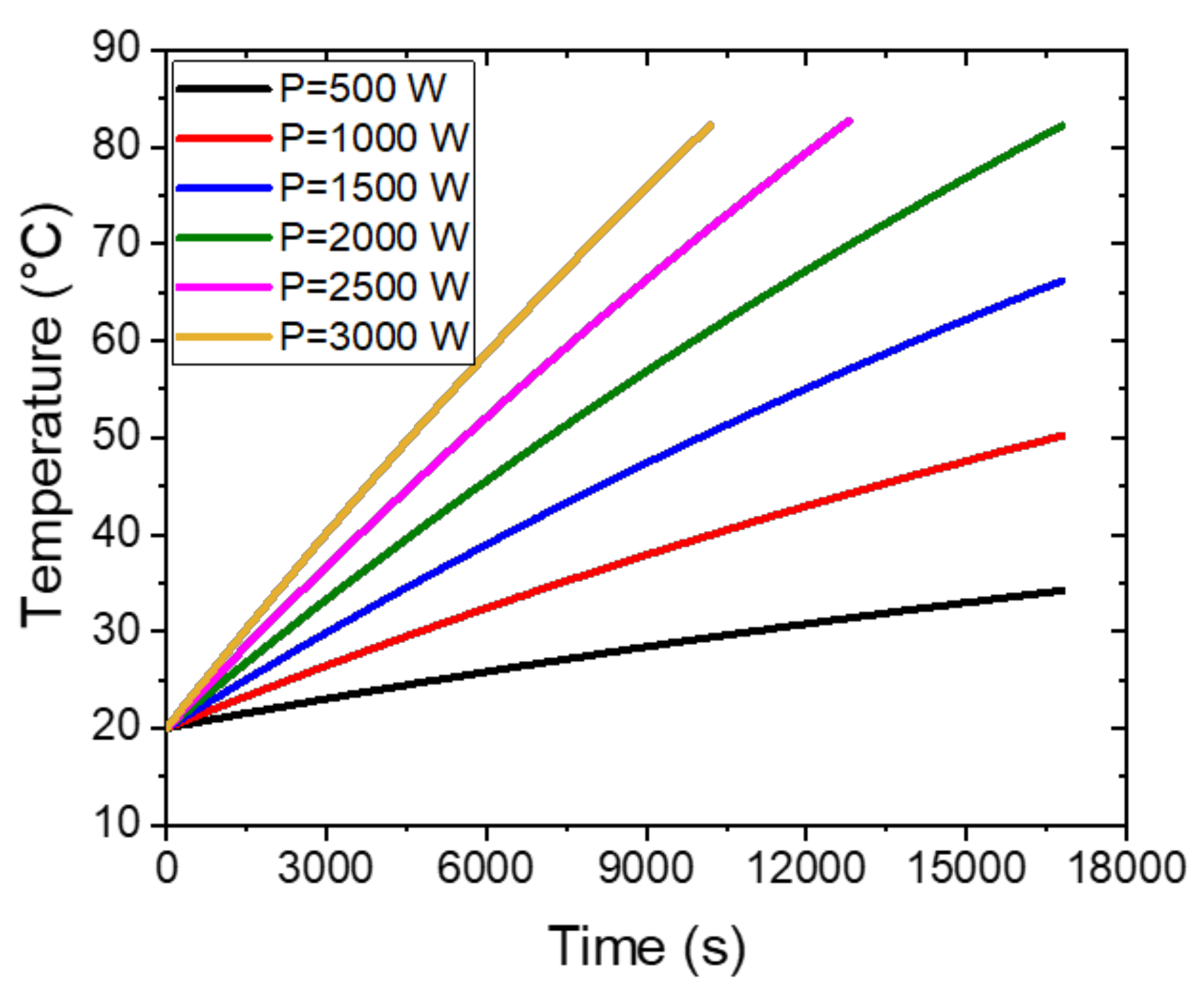
  • The first simulation was achieved with six different electric powers (500, 1000, 1500, 2000, 2500 and 3000 W). The tank had a fixed volume of 100 L with a height of 1050 mm. This choice was made to simulate a typical size of commercial heaters.
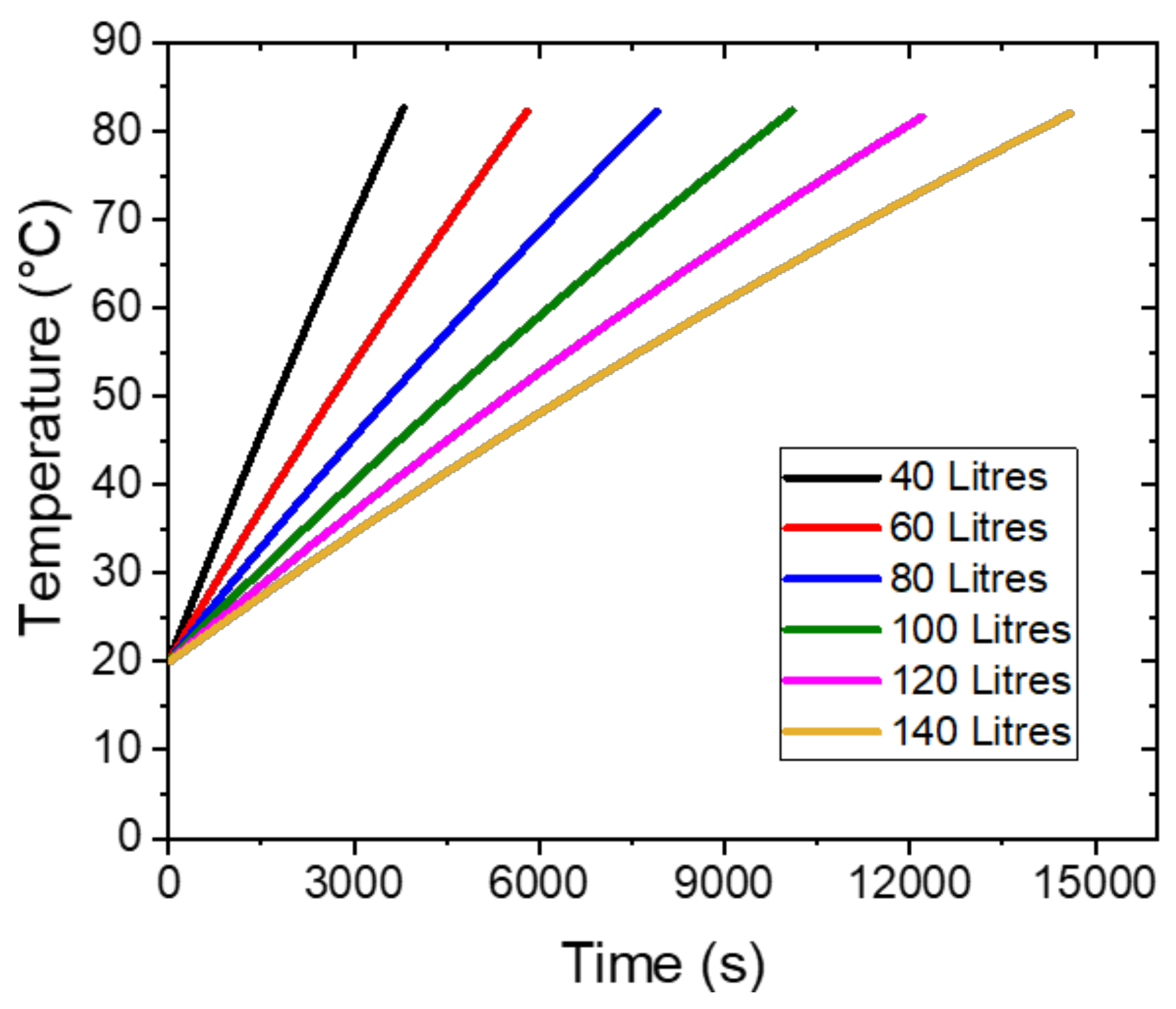
  • The second parameter was the volume of the tank which was varied according to six levels: between 40 and 140 L, conserving a fixed height of 1050 mm. The electrical power was fixed at 3000 Watt. The objective of this study was to quantify the heat losses associated with the change of volume.
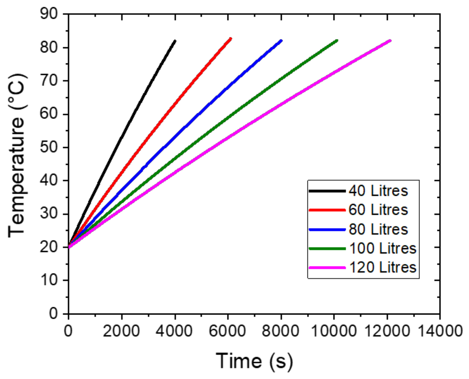
  • The third simulation was designed later and was inspired by the results of the second study which are presented and analyzed in the next paragraph. However, the simulation was based on a variable volume with a constant area of the tank which was fixed at 1.35 m2. This value corresponds to the area of the commercial tank simulated in the first study.
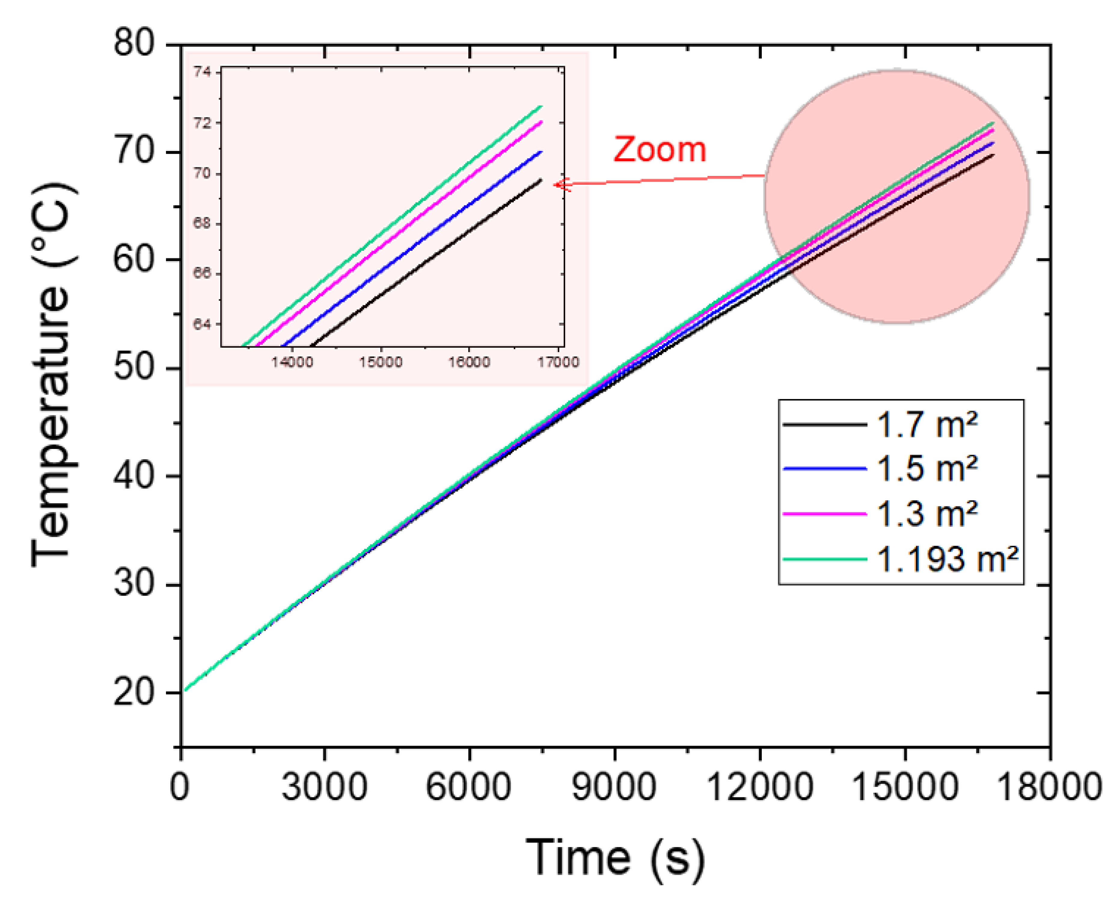
  • The fourth case was done using a fixed power of 3000 W and a fixed volume of 100 L, but with different diameters and heights. The height and diameters were calculated in a manner to obtain 7 different levels of the external area of the tank which were, respectively: 1.193, 1.20, 1.25, 1.30, 1.35, 1.40 and 1.45 m2. The value of 1.193 corresponds to the minimum area which could be obtained for a cylindrical tank of 100 L capacity.

4. Results and Analysis

4.1. Effect of Power

Figure 2 shows the results of the first configuration; it presents the variation of the water temperature in time at different electrical powers. As shown by this figure, when the electrical power increases, the temperature rises faster than expected.
To quantify the effect of the power on the heat losses, one should compare the quantity of heat required to obtain the same thermal state of the tank, namely the same temperature, and this should be done by multiplying the power by the time of heating. Thus, the energy consumption needed to rise the temperature of water to 50 °C for each power is summarized in Table 2.
This table clearly shows that using less power is more energy consuming than using more power. Savings up to 49.7% can be ensured if the heating power is 3 kW instead of 500 W. Furthermore, the desired temperature (50 °C) can be reached in around 1 h and 17 min instead of 15.25 h for the case of 500 Watts. Thus, the optimization can be done according to these observations by increasing the heating power which reduces both heat losses and the time needed to heat the water. However, electric power should be limited with respect to the house installation and to safety standards.
Concerning the heat loss reduction due to increasing the power, it can be explained by two different reasons: First, the reduction of time required to heat the water in the case of rapid heating has a direct effect of the losses which do not have enough time to occur, as in the case of slow heating.
The second reason is behind the performance of the heat exchange itself, which is more powerful in the case of higher heating power due to the higher difference between the water temperature (between 20 °C and 50 °C) and the maximum temperature of water expected at steady state if the time of heating is large enough. For example, the curve of temperature corresponding to 500 W seems to have a maximum not so far from 40 °C, while the curve of 3 kW seems able to reach 200 °C easily. The variable slope of their parts before reaching 50 °C then has to be examined. Indeed, these slopes are globally increased by a factor which is bigger than 3000/500 times when the 500 Watts are replaced by 3000 Watts and this is due to the exponential nature of these curves. This effect explains why the time needed to reach 50 °C in the case of 500 Watts is 3000/500 times larger than the time needed in the case of 3 kW, which explains the higher losses for the case of 500 Watts.

4.2. Effect of Volume

The results of the second configuration are shown in Figure 3. This figure clearly shows that for small volumes the temperature rises faster.
After checking the time needed and the energy consumed to reach a given temperature, i.e., 50 °C, as shown in Table 3, one can compare the case of 40 L and the case of 120 L. More precisely, the consumed energy in the case of 120 L (16,470 kJ) should be compared to the energy consumed in the case of 40 L (5250 kJ). This comparison shows that an energy saving of 4.4% can be obtained if the volume of the tank is divided by three. This result is consistent with the literature [19] but still needs more analyses.
The reason behind higher energy losses in larger tanks can be explained two different ways. The first one is associated with the exponential nature of the ttemperature curves, as explained in the previous paragraph. The second reason is related to the change in the external area of the cylinder. Indeed, the variation of volume with a fixed height of cylinder, as it is the case in this simulation, leads to different external areas. This is why the following simulation was made with a variable volume but a fixed area as a trial to eliminate any interactions between parameters and to show the effect of each parameter independently.

4.3. Effect of Volume under Constant Area

Figure 4 shows the temperature variations with time for the different studied volumes at a constant external area. The same tendencies are observed as in Figure 3 and differences for a same volume cannot be detected easily. Comparisons of time and energy needed to reach 50 °C are shown in Table 4. Comparing the case of 40 L to the case of 120 L, we conclude that the energy saving is now 0.7% instead of 4.4%, as calculated previously. This is an important result showing that the effect of volume on energy losses is mostly an indirect effect due to the variation of cylinder area. However, the volume still has a slight effect on energy losses and small volumes are still recommended.

4.4. Effect of Heater’s External Area

The results of the third configuration are presented in Figure 5. It is clearly shown that the temperature curves of smaller areas are higher than curves of higher areas, and this effect was expected due to the increase of heat losses with the increase of area. A comparison of the consumed energy to reach 50 °C in the case of an area of 1.193 m2 to the case of 1.7 m2 shows that 7.3% of energy can be saved due to the reduction of heat losses.
However, it is fairer to compare the case of minimized area to the case of the commercial heater, as simulated in Section 4.1. The minimized area was obtained for a diameter of 500 mm and a height of 509 mm, whereas the commercial tank has a diameter of 350 mm and a height of 1050 mm. The comparison is given in Figure 6 showing the energy savings that can be obtained if the area is minimized. For instance, by reaching 60 °C a savings of 2.1% can be obtained.
To summarize the effect of the three main studied parameters of power, capacity and external areas, one can compare the energy required to heat 1 Liter of water from 20 °C to 50 °C, as presented in Table 5. Consequently, all these three parameters have a main effect on heater efficiencies and should be taken into consideration when optimizing electrical heaters.

5. Conclusions

The present work concerns an energy investigation related to residential water heating using electricity. A thermal modeling of a typical water heater as well as a relevant experimental method for determining the overall heat transfer coefficient was presented. Calculations with the developed modeling were performed and a parametric study was presented, showing the effects of electric power, tank capacity and tank external area on the efficiency of the heater. It was shown that significant energy savings could be obtained if the power was maximized and the volume was minimized. In the studied intervals of power and volume, energy saving tendencies were shown to have no limits. This means that the saving probably continues to increase until the heater becomes an instantaneous heater when the volume is minimized to its limits and the power is maximized. Finally, the effect of the external area was also quantified, and the study gives a relevant reason to minimize this area for a given volume of the tank.

Author Contributions

Conceptualization, M.K.; methodology, W.S. and M.K.; validation, W.S.; formal analysis, W.S., J.F., E.H., R.M., and M.K.; investigation, W.S., J.F., E.H., R.M., and M.K.; data curation, W.S.; writing—original draft preparation, W.S.; writing—review and editing, J.F., E.H., R.M., and M.K.; supervision, M.K.; project administration, M.K. All authors have read and agreed to the published version of the manuscript.

Funding

The APC was funded by Lebanese International University.

Institutional Review Board Statement

Not applicable.

Informed Consent Statement

Not applicable.

Conflicts of Interest

The authors declare no conflict of interest.

References

  1. Karacan, R.; Mukhtarov, S.; Barış, İ.; İşleyen, A.; Yardımcı, M.E. The impact of oil price on transition toward renewable energy consumption? Evidence from Russia. Energies 2021, 14, 2947. [Google Scholar] [CrossRef]
  2. Sun, R.; Abeynayake, G.; Liang, J.; Wang, K. Reliability and economic evaluation of offshore wind power dc collection systems. Energies 2021, 14, 2922. [Google Scholar] [CrossRef]
  3. Kishore, T.S.; Patro, E.R.; Harish, V.S.K.V.; Haghighi, A.T. A comprehensive study on the recent progress and trends in development of small hydropower projects. Energies 2021, 14, 2882. [Google Scholar] [CrossRef]
  4. Korkeakoski, M. Towards 100% renewables by 2030: Transition alternatives for a sustainable electricity sector in Isla de la Juventud, Cuba. Energies 2021, 14, 2862. [Google Scholar] [CrossRef]
  5. Mehta, K.; Ehrenwirth, M.; Trinkl, C.; Zörner, W.; Greenough, R. The energy situation in Central Asia: A comprehensive energy review focusing on rural areas. Energies 2021, 14, 2805. [Google Scholar] [CrossRef]
  6. Lourenço, J.M.; Aelenei, L.; Sousa, M.; Facão, J.; Gonçalves, H. Thermal behavior of a BIPV combined with water storage: An experimental analysis. Energies 2021, 14, 2545. [Google Scholar] [CrossRef]
  7. Elmouatamid, A.; Ouladsine, R.; Bakhouya, M.; El Kamoun, N.; Khaidar, M.; Zine-Dine, K. Review of control and energy management approaches in micro-grid systems. Energies 2021, 14, 168. [Google Scholar] [CrossRef]
  8. Nall, D. An engineering approach to evaluating energy technology. ASHREA J. 2019, 61, 60–68. [Google Scholar]
  9. Agll, A.A.A.; Hamad, Y.M.; Hamad, T.A.; Sheffield, J.W. Study of energy recovery and power generation from alternative energy source. Case Stud. Therm. Eng. 2014, 4, 92–98. [Google Scholar] [CrossRef] [Green Version]
  10. Chiemchaisri, C.; Juanga, J.P.; Visvanathan, C. Municipal solid waste management in Thailand and disposal emission inventory. Environ. Monit. Assess. 2007, 135, 13–20. [Google Scholar] [CrossRef] [PubMed]
  11. Khaled, M.; Ramadan, M. Heating fresh air by hot exhaust air of HVAC systems. Case Stud. Therm. Eng. 2016, 8, 398–402. [Google Scholar] [CrossRef] [Green Version]
  12. Ramadan, M.; Gad El Rab, M.; Khaled, M. Parametric analysis of air-water heat recovery concept applied to HVAC systems: Effect of mass flow rates. Case Stud. Therm. Eng. 2015, 6, 61–68. [Google Scholar] [CrossRef] [Green Version]
  13. Khaled, M.; Ramadan, M.; Chahine, K.; Assi, A. Prototype implementation and experimental analysis of water heating using recovered waste heat of chimneys. Case Stud. Therm. Eng. 2015, 5, 127–133. [Google Scholar] [CrossRef] [Green Version]
  14. Wannagosit, C.; Sakulchangsatjatai, P.; Kammuang-Lue, N.; Terdtoon, P. Validated mathematical models of a solar water heater system with thermosyphon evacuated tube collectors. Case Stud. Therm. Eng. 2018, 12, 528–536. [Google Scholar] [CrossRef]
  15. Teo, H.G.; Lee, P.S.; Hawlader, M.N.A. An active cooling system for photovoltaic modules. Appl. Energy 2012, 90, 309–315. [Google Scholar] [CrossRef]
  16. Kelly, N.; Strachan, P.A. Modeling enhanced performance inte-grated PV modules. In Proceedings of the 16th European PV SolarEnergy Conference, Glasgow, UK, 1–5 May 2000. [Google Scholar]
  17. Arnaout, M.; Salameh, W.; Assi, A. Impact of solar radiation and temperature levels on the variation of the series and shunt resistors in photovoltaic modules. Int. J. Res. Eng. Technol. 2016, 5, 295–301. [Google Scholar]
  18. Sowmy, D.S.; Prado, R.T.A. Assessment of energy efficiency in electric storage water heaters. In Energy and Buildings; Elsevier B.V.: Amsterdam, The Netherlands, 2008; Volume 40, pp. 2128–2132. [Google Scholar]
  19. Maghami, M.R.; Hizam, H.; Gomes, C.; Radzi, M.A.; Rezadad, M.I.; Hajighorbani, S. Power loss due to soiling on solar panel: A review. Renew. Sustain. Energy Rev. 2016, 59, 1307–1316. [Google Scholar] [CrossRef] [Green Version]
  20. Booysen, M.J.; Engelbrecht, J.A.A.; Molinaro, A. Proof of concept: Large-scale monitor and control of household water heating in near real-time. In Proceedings of the International Conference on Applied Energy, Pretoria, South Africa, 1–4 July 2013. [Google Scholar]
  21. Sateikis, I. Determination of the amount of thermal energy in the tanks of buildings heating systems. In Energy and Buildings; Elsevier: Amsterdam, The Netherlands, 2002; Volume 34, pp. 357–361. [Google Scholar]
  22. Cupelli, L.; Schumacher, M.; Monti, A.; Mueller, D.; De Tommasi, L.; Kouramas, K. Simulation tools and optimization algorithms for efficient energy management in neighborhoods. In Energy Positive Neighborhoods and Smart Energy Districts; Academic Press: Cambridge, MA, USA, 2017; pp. 57–100. [Google Scholar]
  23. Ma, Y.; Kelman, A.; Daly, A.; Borrelli, F. Predictive control for energy efficient buildings with thermal storage: Modeling, stimulation, and experiments. IEEE Control Syst. Mag. 2012, 32, 44–64. [Google Scholar]
  24. O’Dwyer, E.; De Tommasi, L.; Kouramas, K.; Cychowski, M.; Lightbody, G. Modelling and disturbance estimation for model predictive control in building heating systems. In Energy and Buildings; Elsevier: Amsterdam, The Netherlands, 2016; Volume 130, pp. 532–545. [Google Scholar]
  25. O’Dwyer, E.; De Tommasi, L.; Kouramas, K.; Cychowski, M.; Lightbody, G. Prioritised objectives for model predictive control of building heating systems. Control Eng. Pract. 2017, 63, 57–68. [Google Scholar] [CrossRef]
  26. Fiorentini, M.; Wall, J.; Ma, Z.; Braslavsky, J.H.; Cooper, P. Hybrid model predictive control of a residential HVAC system with on-site thermal energy generation and storage. Appl. Energy 2017, 187, 465–479. [Google Scholar] [CrossRef] [Green Version]
  27. Kuboth, S.; Heberle, F.; König-Haagen, A.; Brüggemann, D. Economic model predictive control of combined thermal and electric residential building energy systems. Appl. Energy 2019, 240, 372–385. [Google Scholar] [CrossRef]
Figure 1. Temporal variation of water temperature obtained with the modeling and experiment.
Energies 14 03912 g001
Figure 2. Temporal variation of water temperature for different heat inputs.
Energies 14 03912 g002
Figure 3. Temporal variations of water temperature for different tank capacities.
Energies 14 03912 g003
Figure 4. Temporal variation of water temperature for different tank capacities at a constant area.
Energies 14 03912 g004
Figure 5. Temporal variation of water temperature for different external areas.
Energies 14 03912 g005
Figure 6. Temporal variation of water temperature for tanks with the same capacities and different areas.
Energies 14 03912 g006
Table 1. Parameters of the study.
ConfigurationFixed ParametersVarying Parameters
1 V = 100   L
H = 1050   mm
d = 350   mm
A = 1.35   m 2
500   W P 3000   W
2 P = 3000   W
H = 1050   mm
40   L V 140   L
220   mm d 412   mm
0.803   m 2 A 1.626   m 2
3 P = 3000   W
A = 1.35   m 2
40   L V 120   L  
120   mm d 551   mm
505   mm H 3521   mm
4 P = 3000   W
V = 100   L
1.193   m 2 A 1.450   m 2
307   mm d 500   mm
509   mm H 1347   mm
Table 2. Parameters of the study.
Power
(W)
Time Needed to Reach 50 °C (Seconds)Energy
(kJ)
50054,90027,450
100016,60016,600
150010,00015,000
2000720014,400
2500560014,000
3000460013,800
Table 3. Energy consumption for different tank capacities.
Volume
(Liters)
Time Needed to Reach 50 °C (Seconds)Energy
(kJ)
4017505250
6026507950
80358010,950
100451013,530
120549016,470
140645019,350
Table 4. Energy consumption for different tank capacities.
Volume
(Liters)
Time Needed to Reach 50 °C (Seconds)Energy
(kJ)
4018005400
6027208160
80358010,740
100453013,590
120544016,320
Table 5. Summary of results: potential energy savings.
Energy Required to Reach 50 °CEnergy Savings
Reference configuration:
P = 3000 W
V = 100 L
A = 1.35 m2
138 kJ/L-
P = 500 W
V = 100 L
A = 1.35 m2
274.5 kJ/L−98.9% (losses)
P = 3000 W
V = 40 L
A = 1.35 m2
135 kJ/L2.2% (saving)
P = 3000 W
V = 100 L
A = 1.193 m2
135.1 kJ/L2.1% (saving)
Publisher’s Note: MDPI stays neutral with regard to jurisdictional claims in published maps and institutional affiliations.

