Abstract
The negative impact of transport on climate has led to incentives to increase the amount of renewable fuels used in internal combustion engines (ICEs). Oxygenated, liquid biofuels are promising alternatives, as they exhibit similar combustion behaviour to gasoline. In this article, the effect of the different biofuels on engine efficiency, combustion propagation and emissions of a gasoline-optimised direct injected spark ignited (DISI) engine were evaluated through engine experiments. The experiments were performed without any engine hardware modifications. The investigated fuels are gasoline, four alcohols (methanol, ethanol, n-butanol and iso-butanol) and one ether (MTBE). All fuels were tested at two speed sweeps at low and mid load conditions, and a spark timing sweep at low load conditions. The oxygenated biofuels exhibit increased efficiencies, even at non-knock-limited conditions. At lower loads, the oxygenated fuels decrease CO, HC and NOx emissions. However, at mid load conditions, decreased volatility of the alcohols leads to increased emissions due to fuel impingement effects. Methanol exhibited the highest efficiencies and significantly increased burn rates compared to the other fuels. Gasoline exhibited the lowest level of PN and PM emissions. N-butanol and iso-butanol show significantly increased levels of particle emissions compared to the other fuels.
1. Introduction
The impact of transportation on climate change has caused both global and national incentives to increase the amount of renewable fuels used in internal combustion engines (ICEs) [1,2,3,4,5,6,7]. Liquid biofuels show advantages compared to gaseous alternatives as they exhibit higher energy density and are compatible with current infrastructure [7,8,9]. For utilisation in direct-injected spark-ignited (DISI) engines, oxygenated biofuels (such as alcohols and ethers) are promising as they exhibit similar combustion behaviour to gasoline. Therefore, these fuels require less adaptation for utilisation in existing spark-ignited (SI) engines [7,9,10]. Moreover, the oxygenated biofuels can be blended with gasoline, both at low and high ratios, facilitating the transition from fossil fuels to renewable fuels as production increases [11].
In a previously conducted literature review, it was established that the use of light alcohols, such as ethanol and methanol, in SI engines is well-established and has been investigated for a long time [12]. Light alcohols offers advantages compared to more complex molecules as they can be derived from a variety of process pathways and feedstocks [13,14]. Longer alcohols, such as n-butanol and iso-butanol, have gained interest as a fuel alternative in recent years [12]. Butanols offer similar benefits like the lighter alcohols, but provide higher energy density [15]. Other oxygenated biofuel alternatives are ethers, for example methyl tert-butyl ether (MTBE). MTBE has been used in gasoline as an octane enhancer [16,17] and is produced from methanol and iso-butylene [13]. It is an interesting fuel since its octane ratings are high without a big difference in energy density compared to gasoline. However, MTBE has been restricted in many countries due to its high resistance to biodegradation which affects groundwater aquifers [18]. The above mentioned fuels have been thoroughly investigated for port fuel injected (PFI) SI engines. However, their effect on combustion and emissions in DISI engines is less known. DISI engines have enabled increased engine efficiencies, but they also introduce challenges associated with homogeneous fuel and air mixture preparation, which could lead to increased emission rates of particles [19].
There are several benefits to the utilisation of biofuels in DISI engines, aside from decreased impact on the climate. The main benefit is the increased knock resistance of oxygenated biofuels in comparison with commercial gasoline [3,20,21]. Knock is a major constraint that limits compression ratio (CR), and therefore the efficiency of DISI engines. Biofuels will permit further downsizing and increase in engine efficiency. Most of the oxygenated biofuels exhibit higher octane numbers (RON and MON) compared to gasoline [3,10]. Researchers also report that light alcohols exhibit increased heat of vaporisation (HOV) [9,22,23,24,25] and laminar flame speed (SL) [3,26,27], properties known to benefit knock resistance in engines. Furthermore, gasoline exhibits a negative temperature coefficient (NTC) region, while light alcohols do not [24,28]. The occurrence of an NTC-region facilitates auto-ignition, hence gasoline is more prone to knock compared to alcohols, especially at boosted operation.
Several researchers conclude that biofuels can lead to increased engine efficiency [5,9,11,23,29], increased combustion stability [2,6,30,31], and lower exhaust temperatures [23,32,33] in SI engines. Moreover, due to the increased knock resistance, higher boost pressures can be used to increase peak load of the engine if the engine is optimised for biofuel combustion. Brewster achieved a 13% higher load with ethanol compared to gasoline [34]. Nakata et al. achieved an 11% higher load with ethanol compared to gasoline when the valve timing was optimised [35]. Moreover, several researchers report brake thermal efficiency for ethanol and methanol of 36 to 40% compared to 27 to 36% for gasoline [15,34]. Methanol and ethanol have also shown potential as fuels for heavy-duty (HD) SI application, where similar load and efficiency as HD diesel combustion could be reached with lean combustion of methanol and ethanol [36]. Sileghem et al. showed increased efficiency in comparison to gasoline in a DISI engine fuelled with iso-butanol [15]. The efficiency (brake thermal efficiency) was at the same level as ethanol except for at the highest investigated load (150 Nm). Szwaja and Naber showed that pure n-butanol increased burn rates and indicated efficiency in a single-cylinder CFR engine compared to gasoline [37]. Topgül showed that low level blends of MTBE in gasoline (10% to 30 %) increased brake thermal efficiency, where the highest efficiency was seen for 10% MTBE [38].
It has also been shown that biofuels may lead to decreased emissions from SI engines, such as carbon monoxide (CO) and hydrocarbons (HC) [5,32,39,40]. Masum et al. showed that CO and HC emissions decreased noticeably even at low levels of ethanol and methanol (20%) in the fuel, while a slight decrease was seen for 20% iso-butanol [32]. Sileghem et al. showed that iso-butanol decreased CO, HC and nitrogen oxides (NOx) emissions compared to gasoline in a DISI engine [15]. However, emissions for iso-butanol were higher than for methanol and ethanol. Sandhu et al. showed decreased levels of CO and HC emissions for n-butanol compared to gasoline both at lean and exhaust gas recirculation (EGR) diluted combustion [41]. Schifter et al. concluded that HC and NOx emissions decreased as the volume of MTBE in the fuel increased [33].
Several researchers report the possibility of oxygenated fuels to decrease both particle mass (PM) emissions and particle number (PN) emissions in DISI engines [42,43,44]. The high levels of embedded oxygen in oxygenated biofuels, compared to gasoline, leads to a dilution effect at the flame front. The dilution effect decreases soot formation and increases oxidation rates [45,46,47]. However, oxygenated fuels also exhibit properties that could lead to increased levels of particle emissions, such as decreased volatility, increased HOV and increased viscosity [48]. Thus, early injection could cause increased rates of fuel impingement and pool fires and increase particle emissions compared to gasoline instead [49,50].
Previously conducted research shows great potential for biofuels in future optimised engines. However, the impact of introducing biofuels into already existing gasoline optimised engines needs to be established to facilitate the transition from fossil to renewable fuels. Moreover, the effect of different renewable fuels on engine performance and emissions in different operating points (not only during knock-limited conditions) should be further evaluated to establish their potential as future fuels. Many biofuel alternatives have been tested only as blends with gasoline and not as pure components, and only compared to methanol and/or ethanol. As MTBE has been used mainly as an octane enhancer in gasoline, research evaluating MTBE has focused mainly on blended fuel. Research on MTBE has also decreased, hence few studies on MTBE in DISI engines exist. Furthermore, few studies focus on comparing closely related biofuels, such as iso-butanol and n-butanol, as pure components in production SI engines.
In this article, the engine performance of five pure, liquid, oxygenated biofuels have been evaluated and compared to gasoline through engine experiments. The investigated biofuels are four alcohols (methanol, ethanol, n-butanol and iso-butanol) and one ether (MTBE). The effect of these fuels on engine efficiency, combustion propagation and emissions in a gasoline-optimised DISI engine was investigated under a wide range of engine operating conditions.
2. Materials and Methods
2.1. Experimental Setup
The experiments were conducted on a Volvo Cars T6 DISI engine. The specifications of the test engine can be seen in Table 1. The experiments were performed without any engine hardware modifications. A schematic of the experimental setup can be seen in Figure 1. To measure fuel consumption, an AVL fuel balance (733S) was used for gasoline, ethanol, and n-butanol, and an OHAUS Ranger 7000 scale was used for methanol, iso-butanol, and MTBE.

Table 1.
Specifications of the test engine used, a Volvo Cars T6 DISI engine.
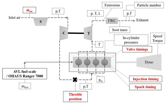
Figure 1.
Schematic of the experimental setup. The dashed boxes are measured using the LabVIEW-system and the variables in red text are measured using signals from the engine control unit. p denotes the measured pressure and T denotes the measured temperature.
Test Fuels
The investigated fuels are gasoline (without any oxygenated additives or compounds) and five single-component oxygenated fuels: ethanol, methanol, n-butanol (nButanol), iso-butanol (iButanol) and methyl tert-butyl ether (MTBE). The properties for these fuels can be seen in Table 2.
Table 2.
Properties of the tested oxygenated biofuels. (* indicates estimated values from [51]).
These fuels were analysed at a commercial laboratory to determine their octane number, lower heating value (LHV) and dry vapour pressure equivalent (DVPE). Research octane number (RON) and motor octane number (MON) for MTBE were estimated using octane numbers from reference [51] since the measured water content was only 0.03%. The gasoline and MTBE were provided by Preem AB, the ethanol by Lantmännen Agroetanol AB, the methanol from Swed Handling AB, and the n-butanol and iso-butanol were provided by Brenntag.
2.2. Methodology
These fuels were tested through two speed sweeps, one at approximately 7.5 bar indicated mean effective pressure (IMEP), and one at approximately 13 bar IMEP. Furthermore, a spark timing sweep was performed at 2500 revolutions per minute (RPM) and approximately 7.5 bar IMEP, see Figure 2. The spark was swept in steps of 2° crank angles (CA) between 14 and 22 crank angle degrees (CAD) before top dead centre (bTDC). An initial stabilisation period of 45 min was applied every time the engine was started and when the fuel had been changed. For each operating point, the engine was stabilised for 15 min. The oil and coolant temperatures were kept at 90–115 °C. Excess air ratio () was kept at 1 ± 0.1. The data was sampled at steady-state, which was identified as the point when the exhaust gas temperature was steady within a range of ±10 °C. The injection duration and injection pressure were adjusted to reach the desired IMEP for each operating point and fuel. For the speed sweeps, the spark timing (ST) was swept until maximum brake torque (MBT) or the knock-limited spark advance (KLSA) was reached. KLSA was defined as the point where the engine control unit (ECU) retarded the spark timing more than 1° CA (using a knock sensor).
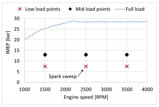
Figure 2.
Engine load in net IMEP (bar) and engine speed (RPM) for the test points.
2.3. Data Acquisition and Analysis
In-cylinder pressure was measured using piezoelectric pressure sensors from Kistler. For each test point, measurements of in-cylinder pressure and inlet gas pressure were retrieved for 150 engine cycles. Measurements of temperatures, pressures, , and emissions were retrieved at 2 Hz for 5 min. The signals from the ECU were collected for 1 min. All specific sensors used and their uncertainties can be seen in Table 3.
Table 3.
Range and uncertainty of the sensors used.
Measurement of exhaust emissions was performed before the three-way catalyst (TWC) using Horiba MEXA-7100 for CO, HC, and NOx, respectively. CO was measured at dry condition, while HC and NOx were measured at wet conditions. was measured using a Bosch wideband oxygen sensor (LSU 4.9).
Particle emissions were measured downstream of the TWC. Soot mass (PM) was measured using an AVL Micro Soot Sensor (MSS) with an internal dilution rate of 1:5. The particle number (PN) was measured using a condensation particle counter from TSI (CPC3010) with a cut-off size of 23 nm. Only non-volatile particle number emissions were measured. The CPC was connected to the exhaust using a two-stage ejector dilution system from Dekati (DI-1000) [52]. The diluter stages were placed in series, where the first diluter stage was heated by incoming dilution air (to approximately 345 °C), while the second diluter stage operated at ambient temperature. The dilution ratio for each diluter was 1:8.45, resulting in a total dilution ratio of 1:71.4. Particle measurements were collected at 1 Hz for 5 min.
The sensor signals were collected using hardware from National Instruments (NI) and a LabVIEW programme developed by the author. All results are presented as mean values. For regulated emissions and particle emissions, the error bars represent standard deviation ().
2.3.1. Calculation of Engine Efficiency and Engine Performance Parameters
The net indicated mean effective pressure (IMEP) is used to indicate the engine load, see Equation (1). The coefficient of variance (COV) and the indicated thermal efficiency (ITE) were both derived using IMEP (Equations (2) and (3)) [53,54].
where V is the calculated in-cylinder volume (m), p is the ensemble averaged in-cylinder pressure pegged against the intake pressure (Pa), is the displacement volume (m), N is the engine speed (rev/s), is the injected fuel mass (kg/s) and is the lower heating value of the fuel (J/kg).
Combustion efficiency () is the ratio between the supplied fuel energy and the released energy. was calculated using the measured concentrations of HC and CO in the exhaust gas. The hydrocarbon emissions reported by the flame ionisation detector (FID) in the exhaust gas analyser (Horiba MEXA-7100) were corrected for the oxygenated fuels to account for the weaker response. The correction factors used can be seen in Table 4 [56]. Combustion efficiency was calculated according to Equation (5) [54,55].
where is the molar mass of HC and CO (g/mol), is the molar mass of the products (g/mol), is the molar fraction of HC and CO, is the molar fraction of water, is the lower heating value of HC and CO, and AFR is the air–fuel ratio.
Table 4.
FID correction factors for HC-emission measurements [56].
2.3.2. Heat Release Analysis and Estimation of Combustion Phasing and Duration
The rate of heat release (ROHR) was calculated using Equation (6). The ratio of specific heats () was calculated using the 7-coefficient NASA polynomials for each fuel [57]. The in-cylinder mass was estimated using the mass flow of fuel and lambda, and the in-cylinder temperature was calculated using the ideal gas law.
ROHR was used to calculate the mass fraction burned (MFB) and find: the flame development angle (CA010), defined as the crank angle between spark and 10% MFB; the combustion duration (CA1090), defined as the crank angle between 10% MFB and 90% MFB; and combustion phasing (CA50), which is the crank angle degree at which 50% of the fuel mass has been burned [53]. In-cylinder pressure, CA010, CA1090, CA50 and ROHR are presented as the assembled average of the measured 150 cycles and based on measured values of cylinder 1 only.
where is the ratio of specific heats, is the rotation angle (CAD) and is the heat transfer to the cylinder walls.
Heat transfer () was estimated using the Woschni model. The heat transfer coefficient was estimated using see Equations (7) and (8) [58]. The average cylinder gas velocity, W (m/s) is given by Equation (9) [59].
where T is the estimated in-cylinder temperature (K), is the wall temperature estimated from the in-cylinder and coolant temperature (K), A is the surface area of the cylinder at the given (), and B is the engine bore (m).
where C1 and C2 are constants which have been calibrated to 1, is the piston speed, is the cylinder volume at inlet valve closing, is the motoring pressure for the engine at the given , is the in-cylinder pressure at inlet valve closing, and is the estimated in-cylinder temperature at inlet valve closing.
2.3.3. Energy Balance Calculation
Energy balance was calculated using Equation (10), where P was calculated using Equation (4), exhaust losses () were calculated using Equation (12), and combustion losses () were calculated using Equation (11) [55]. The specific heat capacity of the exhaust ( and ) was estimated using 7-coefficient NASA polynomials for the exhaust composition, assuming a fully burned stoichiometric fuel/air mixture [57]. Heat losses were assumed to be equal to the difference between the chemical energy of the fuel () and other energy factors (P, and ). The mass flow of air was estimated using the measured fuel consumption and the mean lambda value. The energy balance is based on measured values of cylinder 1 only.
where P, and , and are given in W, is the mass of air (kg/s), is the mean measured exhaust temperature (K), is the specific heat of the exhaust at (J/kg · K), is the specific heat of the exhaust at (J/kg · K) and is the reference temperature (300 K).
2.3.4. Estimation of Laminar Flame Speed
The laminar flame speed () of the test fuels was numerically estimated using CHEMKIN. Laminar flame speed was evaluated for stoichiometric air fuel mixture. Results are presented for a constant engine load and phasing. For this condition, the in-cylinder temperature and pressure were assumed to be constant in the vicinity of the spark plug (regardless of fuel), at 700 K and 10 bar, respectively. The mechanism from Sarathy et al. [60] was used for methanol, ethanol, n-butanol, and iso-butanol. A gasoline surrogate mixture of iso-octane/toluene/1-hexene (50%/35%/15%, respectively) was used with the detailed chemical kinetic mechanism from Mehl et al. [61]. No values of laminar flame speed for MTBE could be found in the literature, thus, values for MTBE have not been estimated.
3. Results and Analysis
3.1. Speed Sweeps at Low and Mid Load Conditions
3.1.1. Engine Efficiency and Engine Performance
The indicated mean effective pressure (IMEP in Figure 3a,b), indicated thermal efficiency (ITE in Figure 3c,d), the coefficient of variance (COV in Figure 3e,f), and the exhaust temperature ( in Figure 3g,h) for the tested fuels can be seen in Figure 3. Gasoline exhibits the lowest IMEP compared to the other fuels (Figure 3a,b). Engine conditions were slightly different when running MTBE tests compared to the other fuels, as MTBE was tested at a marginally higher IMEP than the others.
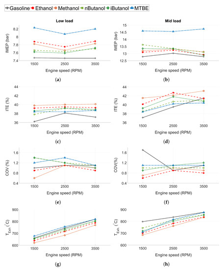
Figure 3.
(a,b) Indicated mean effective pressure (IMEP), (c,d) indicated thermal efficiency (ITE), (e,f) coefficient of variance (COV), and (g,h) exhaust gas temperature () for all tested fuels. Low load conditions to the left and mid load conditions to the right.
Efficiency is higher for the oxygenated fuels compared to gasoline at most tested operating conditions, even at low load when the engine is not limited by knock. Methanol displayed the highest ITE, followed by ethanol. Compared to gasoline, methanol and ethanol improved ITE by 2–4 and 1–3 percentage points, respectively, while n-butanol, iso-butanol and MTBE showed improvements of 1–2 percentage points at some of the tested operating points (the measurement uncertainty was estimated to 0.8 percentage points). The reason for the increased efficiency can be attributed to several properties of the oxygenated biofuels. Since the engine is not knock-limited at low load, the main efficiency gain is not expected to be attributed to the increased knock resistance of the oxygenated fuels compared to gasoline. However, as the alcohols show higher compared to gasoline, this is one of the probable reasons for the increased efficiency, as suggested by Sileghem et al. and Cairns et al. [9,29]. Moreover, an increased cooling effect of the alcohols could lead to lower in-cylinder temperature and thus, decreased heat loss [9].
All of the tested fuels show low levels of combustion instability, see COV in Figure 3e,f. At 1500 RPM and mid load conditions, gasoline exhibits increased COV due to spark retard caused by knock. The lowest COV is seen for methanol and ethanol, while MTBE exhibits the highest COV. As expected, the results indicate that the fuels exhibiting longer flame development time show higher COV, except for gasoline, which exhibits a lower COV than n-butanol. The burn duration also corresponds well to the COV of the different fuels, as supported by the findings of Daniel et al. [62].
The exhaust temperature is displayed in Figure 3g,h. The exhaust temperature increases as engine speed increases. The lowest exhaust temperature is seen from methanol, followed by ethanol, n-butanol, iso-butanol, gasoline and MTBE. This can be connected to the HOV of the fuels, which follows the same trend, with methanol exhibiting the highest heat of vaporisation. Gasoline and n-butanol exhibit higher when they are knock-limited due to retarded combustion phasing.
3.1.2. Combustion Phasing and Duration
Combustion progression for all fuels is represented by the combustion phasing (CA50 in Figure 4a,b), the flame development angle (CA010 in Figure 4c), and the combustion duration (CA1090 in Figure 4e). The results for low load conditions are shown in the left column, while the results at mid load conditions are presented in the right column.
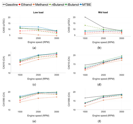
Figure 4.
(a,b) Combustion phasing (CA50), (c,d) flame development angle (CA010) and (e,f) combustion duration (CA1090) for all tested fuels. Low load conditions to the left and mid load conditions to the right.
For low load conditions, the CA50 advances slightly and is closer to TDC when engine speed increases. The increased in-cylinder turbulence at higher speeds may increase the burn rate and cause the advance in CA50. At mid load conditions, CA50 is close to constant at all engine speeds for all fuels except n-butanol and gasoline. At 1500 RPM, gasoline and n-butanol show increased CA50 compared to the other fuels as they were knock-limited at this operating point and MBT could not be achieved. Hence, the applied spark timing was retarded compared to the other fuels. Gasoline was more knock-limited than n-butanol. The other fuels were not knock-limited and MBT could be attained at all engine speeds. Methanol exhibited the lowest CA50 of all the fuels. However, the difference is slightly more pronounced at low load than at mid load conditions.
At both load conditions, CA010 and CA1090 increases as engine speed increases (see Figure 4c,e). However, when engine speed is higher the time per CA is lower. Hence, the longer CA010 and CA1090 could be due to constant combustion duration in time, and not CA, for the fuels.
The flame development angle and the combustion duration differ between fuels. Methanol shows faster combustion propagation compared to the other fuels. The difference is more pronounced at lower load and for CA1090. Methanol exhibits a higher laminar flame speed than gasoline and iso-butanol. However, the reported laminar flame speed (at atmospheric temperature and pressure) for methanol (at ) are at the level of those for ethanol and n-butanol [63,64,65]. Hence, the increased flame propagation of methanol seems to be attributed to other factors, such as in-cylinder conditions, increased injection pressures, and increased injection duration, as methanol exhibits the lowest LHV of all fuels. Another contributing factor could be that more oxygen is readily available in methanol, as the oxygen/carbon (O/C) ratio is high, which have been shown to increase flame propagation [62].
The combustion rates of the other fuels are consistent with the reported laminar flame speed. The burn rates for ethanol and n-butanol are at similar levels. At low load, CA010 at 3500 RPM for n-butanol is marginally shorter than for ethanol, while at 1500 RPM, CA010 is slightly shorter for ethanol. This can be attributed to small changes in the in-cylinder conditions, such as , temperature, and pressure. The burn rates for gasoline, iso-butanol and MTBE are similar, but CA50 for MTBE at low load occurs later. This could be attributed to decreased laminar flame speeds of MTBE, or a difference in in-cylinder conditions at the start of combustion.
3.1.3. Engine Emissions
The regulated engine-out emissions were measured before the TWC. The CO, HC and NOx emissions for both low and mid load conditions can be seen in Figure 5. In Figure 5a,b, the measurement limit is displayed as a dashed line. The values above the threshold have increased uncertainty compared to the data given in Table 3. The error bars are the standard deviation of the measured values ().
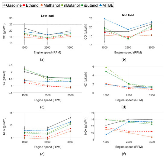
Figure 5.
(a,b) Carbon monoxide (CO) emissions, (c,d) unburned hydrocarbon (HC) emissions and (e,f) nitrogen oxide (NOx) emissions for all tested fuels. Low load conditions to the left and mid load conditions to the right.
3.1.4. Carbon Monoxide Emissions
At low load conditions, CO emissions are lower for the fuels with higher oxygen content, see Figure 5a,b. At stoichiometric conditions CO is a product of incomplete combustion and needs time and a sufficient temperature to be fully oxidised. The oxygenated fuels increase the oxygen ratio in the fuel rich regions of the engine where CO otherwise would form [66,67]. However, at mid load conditions, the trend in CO emissions between fuels is different than at low load conditions. The highest CO emissions are seen for MTBE and gasoline, potentially due to more dissociation of carbon dioxide () at higher loads. Even though MTBE is oxygenated, the increased CO could be due to the higher load in this case. At mid load and 1500 RPM, both n-butanol and iso-butanol show higher levels of CO emissions than gasoline. Furthermore, the emissions of ethanol are close to that of gasoline. The increased levels of CO emissions of these fuels could be explained by the lower volatility of n-butanol, iso-butanol, and ethanol. Low volatility in DISI engines might lead to poor evaporation, pool fires, and locally rich zones, and thus increased CO production. At higher speeds, this effect is not as pronounced as increased in-cylinder temperatures, and in-cylinder turbulence enhances evaporation and fuel/air mixture preparation. Moreover, at higher engine speeds, the injection pressure for the fuels increase as well. In these conditions, the oxygen content of the fuel is the dominant factor affecting CO emissions.
3.1.5. Unburned Hydrocarbon Emissions
The effect of the fuels on the HC emissions is presented in Figure 5c,d. N-butanol and iso-butanol exhibits HC emissions similar to or higher than those of gasoline. At 13 bar IMEP and 1500 RPM, the HC emissions for n-butanol and iso-butanol are significantly higher than for any of the other fuels. At this operating point, ethanol and methanol also show slightly higher HC emissions than gasoline. As for the CO emissions, this could be related to the decreased volatility of these fuels compared to gasoline (see Section 3.1.4). Even if the overall is stoichiometric, fuel impingement creates locally rich zones with incomplete combustion and the formation of HC emissions. However, at higher engine speeds, the difference in HC emissions between the fuels decrease. Higher engine speeds increase in-cylinder turbulence, which might facilitate mixing. Furthermore, at increased engine speeds the temperatures are higher, increasing oxidation rates, and the piston temperature is higher, which increases the evaporation of the fuel pools as well. Evaporation rates and in-cylinder turbulence seem to have a bigger impact for fuels with lower volatility, such as the alcohols, rather than the time available for evaporation and mixing. Furthermore, the oxygenated fuels form hydrocarbon structures that are more reactive than the ones formed from gasoline, which leads to increased oxidation reactivity [45,46,47].
3.1.6. Nitrogen Oxide Emissions
The NOx emissions for low load and mid load conditions can be seen in Figure 5e,f. NOx emissions can be either thermal NOx, prompt NOx, or fuel NOx, where the largest contributor to the NOx emissions formed in ICEs is thermal NOx [68]. Since decreased in-cylinder temperatures reduce the formation of thermal NOx, the fuels with the highest charge cooling capacity exhibited the lowest NOx emissions, as seen in Figure 5e. However, at mid load conditions and 1500 RPM, n-butanol and iso-butanol exhibit the highest level of NOx emissions, and ethanol and methanol exhibit increased levels compared to MTBE, despite having higher HOV. The decreased levels of NOx emissions for gasoline are attributed to increased in-cylinder temperatures due to the retarded combustion phasing caused by knock. A possible explanation for the increased levels of NOx emissions for the alcohols could be the effect of high levels of fuel impingement on the piston at this operating point. As more fuel hits the surfaces inside the cylinder, more fuel is evaporated from the surfaces themselves. Hence, the fuel with high HOV cools the surfaces and not the gas volume in the cylinder. Less cooling of the gas leads to increased in-cylinder temperatures and more NOx. Moreover, the oxygenated fuels could also increase the peak pressure, which leads to higher peak temperatures during combustion, which would also increase the production of thermal NOx.
3.1.7. Particle Emissions
As of 2014 (Euro 6b), particle mass and particle number for SI engines are regulated, and legislation is getting more stringent. Figure 6a shows the soot mass (PM) and Figure 6a shows the particle number (PN) with a cut-off size of 23 nm. In general, the lowest PM and PN are seen for gasoline and not for the oxygenated fuels. The oxygenated fuels were expected to decrease particle emissions, since their chemical structure decreases the formation of soot precursors and increases post-oxidation due to the higher embedded oxygen content [45,69]. However, the formation of particles in ICEs also depends on physical properties, mainly the volatility of the fuel [42,70,71]. Decreased volatility can cause impingement on pistons, cylinder walls and liners leading to pool fires where particles are formed. Hence, poor atomisation and mixing of oxygenated fuels may cause higher particle emissions than for gasoline. This correlates with the results of the HC and CO emissions presented in Figure 5. An increase in both particle number and particle mass suggests that the particles formed are not only in the smaller particle size regime, but there is also accumulation mode particles. At 1500 RPM and mid load conditions, it seems that n-butanol forms a high number of not only nucleation mode particles, but also larger particles affecting the PM emissions. However, a more detailed analysis of the particle size distribution is needed to establish this. Moreover, similar to HC and CO emissions, the PM and PN emissions of n-butanol and iso-butanol drops as engine speed increases. At 3500 RPM, all the fuels exhibit similar PM emissions levels, and more comparable PN emission levels. Another factor increasing the level of particle emissions for the alcohols would be fuel impingement on the cylinder walls, which can increase the amount of oil particles in the cylinder. This could contribute to the increase in PM, but should have a minor effect on PN as oil generally forms larger particles.
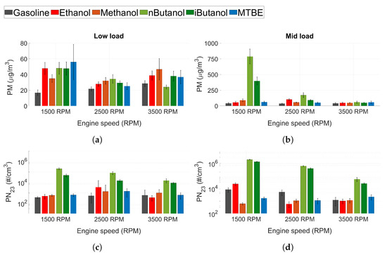
Figure 6.
(a,b) Soot mass (PM) and (c,d) PN (23 nm cut-off) for all tested fuels at low load conditions.
N-butanol exhibited higher levels of PN emissions compared to iso-butanol, even though iso-butanol has a lower DVPE. This could be attributed to the difference in chemical structure between the two fuels. The straight chain chemical structure of n-butanol facilitates the production of soot precursors more than iso-butanol. When engine speed increases, the PN emissions for n-butanol and iso-butanol decreases (like the HC emissions).
3.2. Combustion Propagation at Low Load Conditions
To further evaluate the combustion propagation for the different fuels, a spark-timing sweep between 14 CA bTDC and 22 CA bTDC was performed at low load conditions and 2500 RPM. Figure 7, Figure 8 and Figure 9 are presented for one CA50 for all fuels, at approximately 6 CA after top dead centre (aTDC). The result presented in Figure 10 is evaluated against CA50 for each of the applied spark timings. Results presented in Figure 11 are presented for one CA50 for all fuels, at approximately 6 CA after top dead centre (aTDC). The load and CA50 for each fuel can be seen in Table 5.
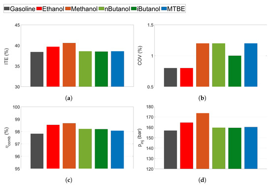
Figure 7.
(a) Indicated thermal efficiency (ITE), (b) coefficient of variance (COV), (c) combustion efficiency () and (d) injection pressure () for all tested fuels at CA50 ≈ 6.
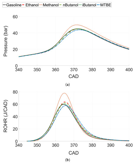
Figure 8.
(a) In-cylinder pressure trace and (b) rate of heat release (ROHR) for all tested fuels at CA50 ≈ 6.
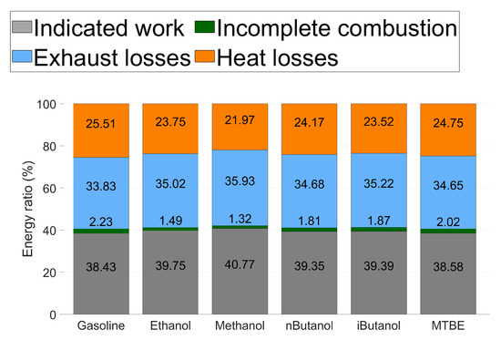
Figure 9.
Energy balance for all tested fuels at CA50 . The percentage for each segment is written in the middle of the coloured segment, incomplete combustion is written above this segment of the bar.
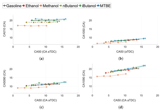
Figure 10.
(a) Flame development angle (CA010), (b) initial burn rate (CA1050), (c) late burn rate (CA5090), and (d) combustion duration (CA1090) for all tested fuels at different CA50.
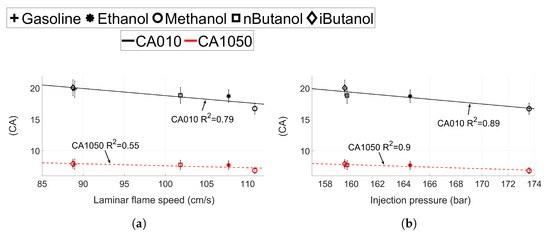
Figure 11.
(a) Laminar flame speed and (b) injection pressure compared to CA10 and CA1050 for gasoline, ethanol, methanol, n-butanol and iso-butanol for CA50 ≈ 6 CA aTDC. CA1090 is displayed in black and CA1050 in red.
3.2.1. Efficiency and Engine Performance Parameters at Constant CA50
Figure 7 shows ITE, COV, combustion efficiency, and injection pressure for all fuels at CA50 . The ITE for methanol and ethanol is slightly higher than for the other fuels at this operating condition (see Figure 7a). Methanol ITE reaches approximately 41%, while the other fuels exhibit ITE below 40%. All fuels exhibit low levels of COV (below 1.3%), see Figure 7b. Methanol, n-butanol and MTBE exhibit the highest COV of all fuels. However the difference between the fuels is less than 1 percentage point, and all fuels exhibit acceptable levels of COV.
The mean combustion efficiency for the tested fuels can be seen in Figure 7c. The alcohols exhibit higher combustion efficiency compared to both MTBE and gasoline. Methanol exhibits the highest combustion efficiency, followed by ethanol. For the light alcohols, the combustion efficiency increases almost 1 percentage point compared to gasoline.
The mean injection pressure for the tested CA50 is displayed in Figure 7d. Methanol has the lowest LHV of all the fuels, hence more methanol needs to be injected to reach the same load compared to other fuels. This leads to an increased injection pressure of methanol. The increased injection pressure of methanol would enhance fuel atomisation and might induce more turbulence into the cylinder, which could explain the increased burn rate and efficiency of methanol, especially compared to ethanol.
3.2.2. Heat Release Analysis and Energy Balance at Constant CA50
To analyse combustion performance, the in-cylinder pressure trace and the estimated rate of heat release (ROHR) are presented in Figure 8 for one CA50 ( 6). Methanol, which showed the highest ITE and combustion efficiency, also shows the highest pressure rise rate and peak pressure (see Figure 8a). Ethanol, n-butanol, iso-butanol and gasoline show similar pressure rise rates, whereas the peak pressure and pressure rise rate for MTBE are slightly lower than for the other fuels. The ROHR shows a similar trend, see Figure 8b. However, even if the pressure trace for ethanol, n-butanol, iso-butanol and gasoline were very similar; there is a slight increase in peak ROHR for the alcohols compared to gasoline. Both ethanol and n-butanol increase the ROHR compared to gasoline, while iso-butanol shows just a slight improvement. Methanol shows a significant increase compared to the other fuels.
The increased ROHR for ethanol and n-butanol compared to gasoline, even if the pressure rise rate is similar, can be explained by decreased heat losses for ethanol and n-butanol as HOV is higher for both fuels. Moreover, Szybist et al. discusses the effect on efficiency of the ratio between the moles of product compared to the moles of reactants at stoichiometric combustion, called the molar expansion ratio (MER) [20]. They explain that for fuels with an increased MER, a higher pressure rise rate compared to other fuels can be distinguished, which enables fuel to produce more indicated work compared to fuels with lower a MER. This would increase ROHR and the efficiency of fuels with a higher MER, such as ethanol and methanol [72].
The energy balance of one CA50 for all the tested fuels is presented in Figure 9. The indicated work is higher and the combustion losses are lower for all of the oxygenated fuels, compared to gasoline. As oxygen content and HOV of the fuel increases, the energy ratio of indicated work increases. Methanol exhibits the highest level of indicated work, which is consistent with the increased ITE of methanol compared to the other fuels. Methanol also exhibits the lowest combustion losses due to incomplete combustion.
Exhaust losses are lower for gasoline than for the oxygenated fuels. Since the oxygenated fuels have lower LHV, there is a higher flow rate in the exhaust as more fuel and air is needed to reach the desired operating point. Increased HOV of the oxygenated fuels decreases the exhaust temperature, but this effect is lower than the increased flow rates.
The heat loss is lower for all of the oxygenated fuels compared to gasoline. Methanol, which exhibits the highest HOV, exhibits the lowest heat loss. This is consistent with the ROHR seen in Figure 8b. As methanol has significantly lower heat losses than the other fuels, it increases ITE and ROHR.
3.2.3. Combustion Phasing and Duration for Different CA50
A more detailed analysis of the burn rates at different stages of the combustion process is shown in Figure 10. It is interesting to note that the flame rate is not heavily affected by the change in CA50 for any of the fuels. Methanol shows a significantly shorter CA010 compared to the other fuels, of approximately 2 CA compared to ethanol and 3 CA compared to gasoline (see Figure 10a). Ethanol and n-butanol exhibit the same CA010, while iso-butanol and gasoline exhibit similar CA010. MTBE is the fuel with the longest flame development angle. N-butanol, methanol, and ethanol exhibits increased laminar flame speeds compared to the other fuels [63,64,65], which correlates well with the shorter CA010 for these fuels compared to iso-butanol, MTBE, and gasoline.
The difference between the fuels for the initial burn rate (CA1050 in Figure 10b) is not as pronounced as for CA010. For all fuels, except methanol, the CA1050 is comparable. The difference between methanol and the other fuels is only approximately 1 CA. The difference between the fuels is even less pronounced at the late stage of combustion (see Figure 10c). The late burn rate (CA5090) is slightly slower than CA1050.
The combustion duration (CA1090) is shown in Figure 10d. Except for methanol, the fuels with a higher laminar flame speed show slightly lower values of CA1090. However, it seems that even though the increased laminar flame speed of methanol, ethanol and n-butanol shows a decrease in the initial part of the combustion (CA010), it does not affect the later stages of combustion significantly. At the later stages the increased injection rates and pressures, due to the decreased energy density of the oxygenated fuels, will have more of an impact on the combustion duration.
The effect of laminar flame speed and the injection pressure on the flame development angle and the initial burn rate can be seen in Figure 11. No values of laminar flame speed for MTBE could be found in the literature, thus values for MTBE are not presented in these graphs.
The coefficient of determination () is 0.79 for the linear correlation between and CA010, but only 0.55 for CA1050, see Figure 11a. The initial flame development is dependent on the laminar flame speed of the fuel, whereas the initial burn rate is not. The results presented in Figure 11b show that while CA010 depends on both laminar flame speed and the injection pressure (), CA1050 shows a correlation only with the injection pressure. These results support the results in Figure 10, where the shorter burn duration for methanol can be correlated to both increased laminar flame speed and increased injection pressures. Hence, it can be concluded that once the flame has been established (after CA10), the in-cylinder turbulence and injection parameters will have more of an impact on the flame propagation than the laminar flame speed.
4. Discussion
The oxygenated biofuels increased both ITE and combustion efficiency compared to gasoline, even though no optimisation has been applied to the engine control, nor the engine hardware. The efficiency increased also if the engine was running at lower loads, where gasoline was not knock-limited. The highest efficiencies were seen for methanol. Furthermore, methanol exhibited a shorter burn duration and increased ROHR compared to the other fuels. Increased efficiencies for methanol was also reported by Sileghem et al. [9]. They did a study of methanol and methanol–water blends in a production SI engine and compared it to gasoline for a high number of operating conditions and compared the performance to gasoline. However, those tests were performed in a port fuel injected engine. Cairns et al. reported increased efficiencies for butanol and ethanol blends in a DISI engine where fuel injection was optimised for the blends [29]. Moreover, the same fuels (gasoline, methanol and ethanol) as used in this study showed great potential as fuel alternatives also in HD SI application [36]. The results in that study were run at a higher compression ratio (13) and thus, more optimised for ethanol and methanol than for gasoline. A future study could investigate if efficiency could be increased even further with increased compression ratios in the light-duty DISI engine used in this study. For MTBE, only results on lower level blends have been reported [38], but it also showed an increased engine efficiency compared to gasoline. Hence, the results in this study add combined information of the performance of different biofuels performed on the same DISI engine at different operating conditions, and in a production engine optimised for gasoline utilisation.
N-butanol was the only oxygenated fuel that was knock-limited. However, a more advanced combustion phasing than that of gasoline could be applied. The RON of n-butanol was slightly higher than for gasoline, but it also has other properties that benefit knock resistance. Increased charge cooling due to higher HOV was shown to mitigate pre-ignition and auto-ignition by Pischinger et al. [24]. Moreover, the shorter combustion duration that was seen for n-butanol, compared to gasoline, also decreases the probability of knock.
As no hardware changes were made to the engine, the same injectors were used for all fuels. Hence, the ECU had to alter injection pressures and injection duration to reach the desired load points. This resulted in a significant increase in injection pressure for methanol compared to the other fuels. The increased injection pressure may increase spray atomization and might improve the in-cylinder turbulence of a spray-guided engine, such as this one. This could affect not only burn rates but also CO, HC and particle formation.
The COV for all fuels were similar to the baseline gasoline and well within the recommended limits for an SI engine. There was no clear trend in COV depending on the properties of the fuels. Daniel et al. [62] noted that combustion instability is reduced due to the increased burn rate of the oxygenated fuels. For low load conditions, ethanol and methanol showed decreased COV compared to the other fuels. However, since the fuel injection in this production engine was calibrated for gasoline, the end of injection varied more when the engine was run with the oxygenated fuels compared to gasoline. This could have had an impact on the COV. Thus, it is possible that with proper fuel injection calibration, the oxygenated fuels would show even lower levels of COV compared to gasoline, corresponding to the shorter CA010. As a result, these fuels could have a higher tolerance for lean or EGR diluted combustion.
The exhaust temperature was lower for the alcohols and showed a good correlation with the increased HOV of the fuels, as supported by previous research [23,32,33]. The charge cooling of the alcohols is beneficial as it lowers in-cylinder temperature and thus heat losses, as could be seen in the performed energy balance. Moreover, if the exhaust gas temperature is lower, it decreases the need for fuel enrichment to protect hardware located in the exhaust stream (turbine and TWC). With this condition, it is possible that the fuels with increased HOV will exhibit an even higher difference in ITE compared to gasoline. Previous studies support the decrease of CO and HC emissions in DISI engines, as the oxygen content of the fuel increases [5,32,39,40]. Sileghem et al. also showed decreased levels of NOx emissions compared to gasoline [15]. In this study, it was shown that the level of emissions depends on the operating conditions, the injection strategy, and the fuel properties. The volatility of the fuel seems to have a higher impact on the engine emissions than the oxygen content, as in this engine, it increases fuel impingement. The effect of injection timing on CO, HC, and NOx emissions could be investigated in a future study.
The low volatility of some of the oxygenated fuels showed a major impact on the particle emissions. Increased levels of PN and PM could be handled by after-treatment systems, such as gasoline particle filters (GPF), or by optimising the fuel injection of the engine. However, researchers have reported increased levels of smaller particles for oxygenated fuels (down to 10 nm) [73], which are harder to trap using a GPF. A more detailed analysis of the particle emissions, including sub-23 nm particles, would give a deeper understanding of the particle emissions from the oxygenated fuels.
5. Conclusions
The implementation of oxygenated biofuels in the current vehicle fleet was investigated by performing tests on a gasoline optimised DISI engine. Five oxygenated biofuels (methanol, ethanol, n-butanol, iso-butanol and MTBE) were tested and compared to gasoline. The fuels were tested at various engine operating conditions: low load and mid load conditions at three different engine speeds and a spark timing sweep was performed at 2500 RPM and 7.5 bar IMEP. The effect of the oxygenated biofuels on engine efficiency, combustion propagation and emissions has been evaluated.
Based on the presented results, the following conclusions were drawn:
- The oxygenated biofuels exhibit increased efficiency at both knock-limited and non-knock-limited engine conditions without any engine or control optimisation.
- Due to increased charge cooling of the alcohols, there is a decrease in heat loss and exhaust temperature compared to gasoline.
- Methanol exhibits significantly increased burn rates compared to the other fuels. This is probably attributed to increased laminar flame speed and higher injection pressures.
- The laminar flame speed seems to have more of an impact during initial flame development (CA010). At the later stages of combustion, in-cylinder turbulence and injection pressure affect flame propagation more.
- The oxygenated fuels, especially methanol and ethanol, decrease emissions of CO, HC and NOx compared to gasoline.
- Gasoline emits the lowest levels of PM and PN emissions.
- N-butanol and iso-butanol show increased levels of particle emissions compared to the other fuels. The low volatility of these fuels leads to high levels of fuel impingement and pool fires. At high load, this also increases HC- and CO emissions. The effect is more pronounced at low speed conditions.
Author Contributions
Conceptualization, T.L., A.C.-E. and U.O.; methodology, T.L., S.K.M. and A.C.-E.; formal analysis, T.L. and S.K.M.; investigation, T.L.; resources, A.C.-E. and U.O.; data curation, T.L. and S.K.M.; writing—original draft preparation, T.L.; writing—review and editing, S.K.M., A.C.-E. and U.O.; visualization, T.L. and S.K.M.; supervision, A.C.-E. and U.O.; project administration, A.C.-E. and U.O.; funding acquisition, A.C.-E. All authors have read and agreed to the published version of the manuscript.
Funding
This work was conducted within the project “Future alternative transportation fuels” and funded by the contributing partners: The Swedish Energy Agency, Chevron, Lantmännen, Perstorp AB, Preem, Scania CV AB, St1, Saybolt Sweden, Stena Line, Volvo AB and Volvo Cars.
Institutional Review Board Statement
Not applicable.
Informed Consent Statement
Not applicable.
Data Availability Statement
Not applicable.
Acknowledgments
The authors would like to thank Volvo Cars for their help and support during the project. The authors would also like to thank Saybolt Sweden AB for performing the fuel tests, and Preem and Lantmännen for providing the fuel used for the experiments.
Conflicts of Interest
The authors declare no conflict of interest.
Abbreviations
The following abbreviations are used in this manuscript:
| Ratio of specific heats | |
| Combustion efficiency | |
| Standard deviation | |
| Excess air ratio | |
| A | Area |
| AFR | Air-fuel ratio |
| aTDC | After top dead centre |
| B | Engine bore |
| bTDC | Before top dead centre |
| CA | Crank angle |
| CA010 | Flame development angle |
| CA1050 | Initial burn rate |
| CA1090 | Combustion duration |
| CA50 | Combustion phasing |
| CA5090 | Late burn rate |
| CAD | Crank angle degree |
| CO | Carbon monoxide |
| COV | Coefficient of variance |
| Specific heat capacity | |
| CPC | Condensation particle counter |
| CR | Compression ratio |
| DISI | Direct-injected spark-ignited |
| DVPE | Dry vapour pressure equivalent |
| ECU | Engine control unit |
| EGR | Exhaust gas recirculation |
| FID | Flame ionisation detector |
| FS | Full scale (uncertainty) |
| GPF | Gasoline particulate filter |
| HC | Hydrocarbon |
| HD | Heavy duty |
| HOV | Heat of vaporisation |
| ICE | Internal combustion engine |
| IMEP | Indicated mean effective pressure |
| ITE | Indicated thermal efficiency |
| KLSA | knock-limited spark advance |
| LHV | Lower heating value |
| Air mass flow | |
| MER | Molar expansion ratio |
| MBT | Maximum brake torque |
| MFB | Mass fraction burned |
| Fuel mass flow | |
| MON | Motor octane number |
| MSS | Micro soot sensor |
| MTBE | Methy tert-butyl ether |
| N | Engine speed |
| NASA | National Aeronautics and Space Administration |
| NI | National Instruments |
| NOx | Nitrogen oxide |
| NTC | Negative temperature coefficient |
| O/C | Oxygen to carbon ratio |
| p | In-cylinder pressure |
| PFI | Port fuel injection |
| Injection pressure | |
| PM | Particle (soot) mass |
| Motoring pressure | |
| PN | Particle number |
| P | Net indicated power |
| Combustion energy loss | |
| Exhaust gas loss | |
| Lower heating value | |
| Coefficient of determination | |
| RPM | Revolution per minute |
| ROHR | Rate of heat release |
| RON | Research octane number |
| SI | Spark-ignited |
| Laminar flame speed | |
| SOC | Start of combustion |
| Piston speed | |
| ST | Spark timing |
| T | In-cylinder temperature |
| Exhaust gas temperature | |
| Wall temperature | |
| TWC | Three-way catalyst |
| V | In-cylinder volume |
| Displacement volume |
References
- Brownstein, A.M. (Ed.) History and Legislation. In Renewable Motor Fuels; Elsevier Inc.: Amsterdam, The Netherlands, 2015; Chapter 1; pp. 1–8. [Google Scholar] [CrossRef]
- Pearson, R.J.; Turner, J.W.G. Renewable Fuels: An Automotive Perspective. In Comprehensive Renewable Energy; Sayigh, A., Ed.; Elsevier: Amsterdam, The Netherlands, 2012; pp. 305–342. [Google Scholar] [CrossRef]
- Bergthorson, J.M.; Thomson, M.J. A review of the combustion and emissions properties of advanced transportation biofuels and their impact on existing and future engines. Renew. Sustain. Energy Rev. 2014, 42, 1393–1417. [Google Scholar] [CrossRef]
- Arce-Alejandro, R.; Villegas-Alcaraz, J.F.; Gómez-Castro, F.I.; Juárez-Trujillo, L.; Sánchez-Ramírez, E.; Carrera-Rodríguez, M.; Morales-Rodríguez, R. Performance of a gasoline engine powered by a mixture of ethanol and n-butanol. Clean Technol. Environ. Policy 2018, 20, 1929–1937. [Google Scholar] [CrossRef]
- Wang, C.; Herreros, J.M.; Jiang, C.; Sahu, A.; Xu, H. Engine Thermal Efficiency Gain and Well-to-Wheel Greenhouse Gas Savings When Using Bioethanol as a Gasoline-Blending Component in Future Spark-Ignition Engines: A China Case Study. Energy Fuels 2018, 32, 1724–1732. [Google Scholar] [CrossRef]
- Yusoff, M.N.A.M.; Zulkifli, N.W.M.; Masum, B.M.; Masjuki, H.H. Feasibility of bioethanol and biobutanol as transportation fuel in spark-ignition engine: A review. RSC Adv. 2015, 5, 100184–100211. [Google Scholar] [CrossRef]
- Sarathy, M.; Oßwald, P.; Hansen, N.; Kohse-Höinghaus, K. Alcohol combustion chemistry. Prog. Energy Combust. Sci. 2014, 44, 40–102. [Google Scholar] [CrossRef]
- Kalghatgi, G.; Stone, R. Fuel Requirements of spark ignition engines. Proc. Inst. Mech. Eng. Part D J. Automob. Eng. 2017. [Google Scholar] [CrossRef]
- Sileghem, L.; Huylebroeck, T.; den Bulcke, A.; Vancoillie, J.; Verhelst, S. Performance and Emissions of a SI Engine using Methanol-Water Blends; SAE Technical Papers; SAE International: Warrendale, PA, USA, 2013. [Google Scholar] [CrossRef]
- Westbrook, C.K. Biofuels Combustion. Annu. Rev. Phys. Chem. 2013, 64, 201–219. [Google Scholar] [CrossRef]
- Turner, J.; Lewis, A.; Akehurst, S.; Brace, C.J.; Verhelst, S.; Vancoillie, J.; Sileghem, L.; Leach, F.C.; Ewards, P.P. Alcohol Fuels for Spark-Ignition Engines: Performance, Efficiency and Emission Effects at Mid to High Blend Rates for Ternary Mixtures. Energies 2020, 13, 6390. [Google Scholar] [CrossRef]
- Larsson, T.; Erlandsson, A.C.; Stenlåås, O. Future Fuels for DISI Engines: A Review on Oxygenated, Liquid Biofuels; SAE Technical Papers; SAE International: Warrendale, PA, USA, 2019. [Google Scholar] [CrossRef]
- Moulijn, J.A.; Makkee, M.; van Diepen, A.E. Biotechnology. In Chemical Process Technology, 2nd ed.; Wiley: Hoboken, NJ, USA, 2013; pp. 423–452. [Google Scholar]
- Dabelstein, W.; Reglitzky, A.; Schütze, A.; Reders, K. Automotive Fuels. In Ullmann’s Encyclopedia of Industrial Chemistry; American Cancer Society: Atlanta, GA, USA, 2007. [Google Scholar] [CrossRef]
- Sileghem, L.; Ickes, A.; Wallner, T.; Verhelst, S. Experimental Investigation of a DISI Production Engine Fuelled with Methanol, Ethanol, Butanol and ISO-Stoichiometric Alcohol Blends; SAE Technical Papers; SAE International: Warrendale, PA, USA, 2015. [Google Scholar] [CrossRef]
- Rosell, M.; Lacorte, S.; Barceló, D. Analysis, occurrence and fate of MTBE in the aquatic environment over the past decade. Trends Anal. Chem. TRAC 2006, 25, 1016–1029. [Google Scholar] [CrossRef]
- Schifter, I.; Gonzàlez, U.; Dìaz, L.; Gonzàlez-Macìas, C.; Mejìa-Centeno, I. Experimental and vehicle (on road) test investigations of spark-ignited engine performance and emissions using high concentration of MTBE as oxygenated additive. Fuel 2017, 187, 276–284. [Google Scholar] [CrossRef]
- Squillace, P.J.; Pankow, J.F.; Korte, N.E.; Zogorski, J.S. Review of the environmental behavior and fate of methyl tert-butyl ether. Environ. Toxicol. Chem. 1997, 16, 1836–1844. [Google Scholar] [CrossRef]
- Leach, F.; Knorsch, T.; Laidig, C.; Wiese, W. A Review of the Requirements for Injection Systems and the Effects of Fuel Quality on Particulate Emissions from GDI Engines. In Proceedings of the International Powertrains, Fuels & Lubricants Meeting, Heidelberg, Germany, 17–19 September 2018; SAE International: Warrendale, PA, USA, 2018. [Google Scholar] [CrossRef]
- Szybist, J.P.; Chakravathy, K.; Daw, C.S. Analysis of the Impact of Selected Fuel Thermochemical Properties on Internal Combustion Engine Efficiency. Energy Fuels 2012, 26, 2798–2810. [Google Scholar] [CrossRef]
- Singh, E.; Morganti, K.; Dibble, R. Knock and Pre-Ignition Limits on Utilization of Ethanol in Octane-on-Demand Concept; SAE Technical Papers; SAE International: Warrendale, PA, USA, 2019. [Google Scholar] [CrossRef]
- Turner, D.; Xu, H.; Cracknell, R.F.; Natarajan, V.; Chen, X. Combustion performance of bio-ethanol at various blend ratios in a gasoline direct injection engine. Fuel 2011, 90, 1999–2006. [Google Scholar] [CrossRef]
- Catapano, F.; Di Iorio, S.; Sementa, P.; Vaglieco, B.M. Characterization of Ethanol-Gasoline Blends Combustion Processes and Particle Emissions in a GDI/PFI Small Engine; SAE Technical Papers; SAE International: Warrendale, PA, USA, 2014. [Google Scholar] [CrossRef]
- Pischinger, S.; Günther, M.; Budak, O. Abnormal combustion phenomena with different fuels in a spark ignition engine with direct fuel injection. Combust. Flame 2017, 175, 123–137. [Google Scholar] [CrossRef]
- Wei, H.; Feng, D.; Pan, M.; Pan, J.; Rao, X.; Gao, D. Experimental investigation on the knocking combustion characteristics of n-butanol gasoline blends in a DISI engine. Appl. Energy 2016, 175, 346–355. [Google Scholar] [CrossRef]
- Wu, F.; Law, C.K. An experimental and mechanistic study on the laminar flame speed, Markstein length and flame chemistry of the butanol isomers. Combust. Flame 2013, 160, 2744–2756. [Google Scholar] [CrossRef]
- Broustail, G.; Seers, P.; Halter, F.; Moréac, G.; Mounaim-Rousselle, C. Experimental determination of laminar burning velocity for butanol and ethanol iso-octane blends. Fuel 2011, 90, 1–6. [Google Scholar] [CrossRef]
- Bogin, G.E., Jr.; Luecke, J.; Ratcliff, M.A.; Osecky, E.; Zigler, B.T. Effects of iso-octane/ethanol blend ratios on the observance of negative temperature coefficient behavior within the Ignition Quality Tester. Fuel 2016, 186, 82–90. [Google Scholar] [CrossRef]
- Cairns, A.; Stansfield, P.; Fraser, N.; Blaxill, H.; Gold Martin Rogerson, J.; Goodfellow, C. A Study of Gasoline-Alcohol Blended Fuels in an Advanced Turbocharged DISI Engine. SAE Int. J. Fuels Lubr. 2009, 2, 41–57. [Google Scholar] [CrossRef][Green Version]
- Yanowitz, J.; Christensen, E.; McCormick Robert, L. Utilization of Renewable Oxygenates as Gasoline Blending Components; Technical Report; National Renewable Energy Laboratory: Golden, CO, USA, 2011.
- Westphal, G.; Krahl, J.; Brüning, T.; Hallier, E.; Bünger, J. Ether oxygenate additives in gasoline reduce toxicity of exhausts. Toxicology 2010, 268, 198–203. [Google Scholar] [CrossRef]
- Masum, B.M.; Kalam, M.A.; Masjuki, H.H.; Palash, S.M.; Fattah, I.M.R. Performance and emission analysis of a multi cylinder gasoline engine operating at different alcohol gasoline blends. RSC Adv. 2014, 4, 27898–27904. [Google Scholar] [CrossRef]
- Schifter, I.; González, U.; González-Macías, C. Effects of ethanol, ethyl-tert-butyl ether and dimethyl-carbonate blends with gasoline on SI engine. Fuel 2016, 183, 253–261. [Google Scholar] [CrossRef]
- Brewster, S. Initial Development of a Turbo-Charged Direct Injection E100 Combustion System; SAE Technical Papers; SAE International: Warrendale, PA, USA, 2007. [Google Scholar] [CrossRef]
- Nakata, K.; Utsumi, S.; Ota, A.; Kawatake, K.; Kawai, T.; Tsunooka, T. The Effect of Ethanol Fuel on a Spark Ignition Engine; SAE Technical Papers; SAE International: Warrendale, PA, USA, 2006. [Google Scholar] [CrossRef]
- Mahendar, S.K.; Larsson, T.; Erlandsson, A.C. Alcohol lean burn in heavy duty engines: Achieving 25 bar IMEP with high efficiency in spark ignited operation. Int. J. Engine Res. 2020, 1468087420972897. [Google Scholar] [CrossRef]
- Szwaja, S.; Naber, J. Combustion of n-butanol in a spark-ignition IC engine. Fuel 2010, 89, 1573–1582. [Google Scholar] [CrossRef]
- Topgül, T. The effects of MTBE blends on engine performance and exhaust emissions in a spark ignition engine. Fuel Process. Technol. 2015, 138. [Google Scholar] [CrossRef]
- Masum, B.M.; Masjuki, H.H.; Kalam, M.A.; Palash, S.M.; Habibullah, M. Effect of alcohol–gasoline blends optimization on fuel properties, performance and emissions of a SI engine. J. Clean. Prod. 2015, 86, 230–237. [Google Scholar] [CrossRef]
- Anselmi, P.; Matrat, M.; Starck, L.; Duffour, F. Combustion characteristics of oxygenated fuels Ethanol-and Butanol-gasoline fuel blends, and their impact on performance, emissions and Soot Index. In Proceedings of the 2019 JSAE/SAE Powertrains, Fuels and Lubricants, Kyoto, Japan, 26–29 August 2019; SAE International: Warrendale, PA, USA, 2019. [Google Scholar] [CrossRef]
- Sandhu, N.S.; Yu, X.; Leblanc, S.; Zheng, M.; Ting, D.; Li, T. Combustion Characterization of Neat n-Butanol in an SI Engine. In Proceedings of the WCX SAE World Congress Experience, Detroit, Michigan, 5–7 April 2020; SAE International: Warrendale, PA, USA, 2020. [Google Scholar] [CrossRef]
- Di Iorio, S.; Lazzaro, M.; Sementa, P.; Vaglieco, B.M.; Catapano, F. Use of Renewable Oxygenated Fuels in Order to Reduce Particle Emissions from a GDI High Performance Engine; SAE International: Warrendale, PA, USA, 2011. [Google Scholar] [CrossRef]
- Karavalakis, G.; Short, D.; Vu, D.; Russell, R.L.; Asa-Awuku, A.; Jung, H.; Johnson, K.C.; Durbin, T.D. The impact of ethanol and iso-butanol blends on gaseous and particulate emissions from two passenger cars equipped with spray-guided and wall-guided direct injection SI (spark ignition) engines. Energy 2015, 82, 168–179. [Google Scholar] [CrossRef]
- Qin, J.; Li, X.; Pei, Y. Effects of Combustion Parameters and Lubricating Oil on Particulate Matter Emissions from a Turbo-Charged GDI Engine Fueled with Methanol/Gasoline Blends. In Proceedings of the SAE 2014 International Powertrain, Fuels & Lubricants Meeting, Birmingham, UK, 20–23 October 2014; SAE International: Warrendale, PA, USA, 2014. [Google Scholar] [CrossRef]
- Ferraro, F.; Russo, C.; Schmitz, R.; Hasse, C.; Sirignano, M. Experimental and numerical study on the effect of oxymethylene ether-3 (OME3) on soot particle formation. Fuel 2021, 286, 119353. [Google Scholar] [CrossRef]
- Wei, J.; Zeng, Y.; Pan, M.; Zhuang, Y.; Qiu, L.; Zhou, T.; Liu, Y. Morphology analysis of soot particles from a modern diesel engine fueled with different types of oxygenated fuels. Fuel 2020, 267, 117248. [Google Scholar] [CrossRef]
- Verma, P.; Jafari, M.; Rahman, S.A.; Pickering, E.; Stevanovic, S.; Dowell, A.; Brown, R.; Ristovski, Z. The impact of chemical composition of oxygenated fuels on morphology and nanostructure of soot particles. Fuel 2020, 259, 116167. [Google Scholar] [CrossRef]
- Chen, H.; Xu, M.; Zhang, G.; Zhang, M.; Zhang, Y. Investigation of Ethanol Spray From Different DI Injectors by Using Two-Dimensional Laser Induced Exciplex Fluorescence at Potential Cold-Start Condition. In Proceedings of the ASME 2010 Internal Combustion Engine Division Fall Technical Conference, San Antonio, TX, USA, 12–15 September 2010. [Google Scholar] [CrossRef]
- Bonatesta, F.; Chiappetta, E.; La Rocca, A. Part-load particulate matter from a GDI engine and the connection with combustion characteristics. Appl. Energy 2014, 124, 366–376. [Google Scholar] [CrossRef]
- Larsson, T.; K, A.P.; Olofsson, U.; Erlandsson, A. Undiluted Measurement of sub 10 nm Non-Volatile and Volatile Particle Emissions from a DISI Engine Fueled with Gasoline and Ethanol; SAE International: Warrendale, PA, USA, 2021. [Google Scholar] [CrossRef]
- Babazadeh Shayan, S.; Seyedpour, S.M.; Ommi, F. Effect of oxygenates blending with gasoline to improve fuel properties. CJME 2012, 25, 792–797. [Google Scholar] [CrossRef]
- Dekati. Dekati Diluter. 2020. Available online: https://dekatitechnologies.com/?gclid=EAIaIQobChMI5tWR3K688QIVmulRCh03ZwgYEAAYASAAEgKRivD_BwE (accessed on 10 December 2020).
- Heywood, J.B. Combustion in Spark-Ignition Engines. In Internal Combustion Engine Fundamentals, 2nd ed.; McGraw-Hill Education: New York, NY, USA, 1988. [Google Scholar]
- Heywood, J.B. Engine Design and Operating Parameters. In Internal Combustion Engine Fundamentals, 2nd ed.; McGraw-Hill Education: New York, NY, USA, 1988. [Google Scholar]
- Bengt, J. Engine Efficiency and pressures. In Combustion Engines Part I; Department of Energy Sciences; Lund University: Lund, Sweden, 2014. [Google Scholar]
- Wallner, T. Correlation Between Speciated Hydrocarbon Emissions and Flame Ionization Detector Response for Gasoline/Alcohol Blends. ASME J. Eng. Gas Turbines Power 2011, 133. [Google Scholar] [CrossRef]
- Burcat, A.; Ruscic, B. Third Millennium Ideal Gas and Condensed Phase Thermochemical Database for Combustion with Updates from Active Thermochemical Tables; Technical Report; U.S. Department of Energy: Oak Ridge, TN, USA, 2005. [CrossRef]
- Heywood, J.B. Engine Heat Transfer. In Internal Combustion Engine Fundamentals, 2nd ed.; McGraw-Hill Education: New York, NY, USA, 1988. [Google Scholar]
- Maurya, R.K. Combustion Characteristic Analysis. In Reciprocating Engine Combustion Diagnostics: In-Cylinder Pressure Measurement and Analysis; Springer International Publishing: Cham, Switzerland, 2019; pp. 281–359. [Google Scholar] [CrossRef]
- Sarathy, S.; Vranckx, S.; Yasunaga, K.; Mehl, M.; Oßwald, P.; Metcalfe, W.; Westbrook, C.; Pitz, W.; Kohse-Höinghaus, K.; Curran, H. A comprehensive chemical kinetic combustion model for the four butanol isomers. Combust. Flame 2012, 159, 2028–2055. [Google Scholar] [CrossRef]
- Mehl, M.; Pitz, W.J.; Westbrook, C.K.; Curran, H.J. Kinetic modeling of gasoline surrogate components and mixtures under engine conditions. Proc. Combust. Inst. 2011, 33, 193–200. [Google Scholar] [CrossRef]
- Daniel, R.; Tian, G.; Xu, H.; Shuai, S. Ignition timing sensitivities of oxygenated biofuels compared to gasoline in a direct-injection SI engine. Fuel 2012, 99, 72–82. [Google Scholar] [CrossRef]
- Veloo, P.S.; Egolfopoulos, F.N. Flame propagation of butanol isomers/air mixtures. Proc. Combust. Inst. 2011, 33, 987–993. [Google Scholar] [CrossRef]
- Veloo, P.S.; Wang, Y.L.; Egolfopoulos, F.N.; Westbrook, C.K. A comparative experimental and computational study of methanol, ethanol, and n-butanol flames. Combust. Flame 2010, 157, 1989–2004. [Google Scholar] [CrossRef]
- Sileghem, L.; Alekseev, V.; Vancoillie, J.; Nilsson, E.; Verhelst, S.; Konnov, A. Laminar burning velocities of primary reference fuels and simple alcohols. Fuel 2014, 115, 32–40. [Google Scholar] [CrossRef]
- Iodice, P.; Senatore, A.; Langella, G.; Amoresano, A. Effect of ethanol–gasoline blends on CO and HC emissions in last generation SI engines within the cold-start transient: An experimental investigation. Appl. Energy 2016, 179, 182–190. [Google Scholar] [CrossRef]
- Shahad, H.A.K.; Wabdan, S.K. Effect of Operating Conditions on Pollutants Concentration Emitted from a Spark Ignition Engine Fueled with Gasoline Bioethanol Blends. J. Renew. Energy 2015, 2015, 170896. [Google Scholar] [CrossRef]
- Bengt, J. Spark Ignition Engine Emissions. In Combustion Engines Part I; Department of Energy Sciences, Lund University: Lund, Sweden, 2014. [Google Scholar]
- Hua, Y.; Liu, F.; Qiu, L.; Qian, Y.; Meng, S. Numerical study of particle dynamics in laminar diffusion flames of gasoline blended with different alcohols. Fuel 2019, 257, 116065. [Google Scholar] [CrossRef]
- Wang, C.; Xu, H.; Herreros, J.M.; Wang, J.; Cracknell, R. Impact of fuel and injection system on particle emissions from a GDI engine. Appl. Energy 2014, 132, 178–191. [Google Scholar] [CrossRef]
- Raza, M.; Chen, L.; Leach, F.; Ding, S. A Review of Particulate Number (PN) Emissions from Gasoline Direct Injection (GDI) Engines and Their Control Techniques. Energies 2018, 6, 1417. [Google Scholar] [CrossRef]
- Nguyen, D.K.; Szybist, J.; Sileghem, L.; Verhelst, S. Effects of molar expansion ratio of fuels on engine efficiency. Fuel 2020, 263, 116743. [Google Scholar] [CrossRef]
- Yu, X.; Guo, Z.; He, L.; Dong, W.; Sun, P.; Shi, W.; Du, Y.; He, F. Effect of gasoline/n-butanol blends on gaseous and particle emissions from an SI direct injection engine. Fuel 2018, 229, 1–10. [Google Scholar] [CrossRef]


Publisher’s Note: MDPI stays neutral with regard to jurisdictional claims in published maps and institutional affiliations. |
© 2021 by the authors. Licensee MDPI, Basel, Switzerland. This article is an open access article distributed under the terms and conditions of the Creative Commons Attribution (CC BY) license (https://creativecommons.org/licenses/by/4.0/).