Abstract
This paper presents a procedure for the derivation of an equivalent thermal network-based model applied to three-core armored submarine cables. The heat losses of the different metallic cable parts are represented as a function of the corresponding temperatures and the conductor current, using a curve-fitting technique. The model was applied to two cables with different filler designs, supposed to be equipped with distributed temperature sensing (DTS) and the optical fiber location in the equivalent circuit was adjusted so that the conductor temperature could be accurately estimated using the sensor measurements. The accuracy of the proposed model was tested for both stationary and dynamic loading conditions, with the corresponding simulations carried out using a hybrid 2D-thermal/3D-electromagnetic model and the finite element method for the numerical resolution. Mean relative errors between 1 and 3% were obtained using an actual current profile. The presented procedure can be used by cable manufacturers or by utilities to properly evaluate the cable thermal situation.
1. Introduction
In recent decades, the number of projects and installed capacities involving submarine power cables have significantly increased. Most of these are devoted to connecting offshore wind power plants (OWPPs) to the onshore grid (e.g., in Europe, the cumulative installed capacity was raised from 2 GW in 2009 to 22 GW in 2019 [1]), while others are related to underwater HV interconnection links (e.g., inland to islands, between islands). Future plans to install new HV OWPPs show that this trend is increasing, as in the case of Europe, where the annual installation rate is expected to be doubling in the following years [1]. In this sense, design features like cable current ratings higher than 1500 A or cable lengths higher than 100 km are nowadays not infrequent [2].
One of the most critical parts of this kind of infrastructure is the power cable; therefore, it must be adequately designed and operated to prevent costly failures and repair costs. In this sense, much effort has been devoted in recent years to increasing the possibilities for its condition monitoring, allowing the early detection of incipient failures or misoperation risk beyond thermal/mechanical limits [3]. Distributed temperature sensing (DTS) is one of these techniques, commercially available since the 1990s for land-extruded HV cables, which has become widespread in recent years for submarine cables [4]. It measures the temperature along part of or the whole cable (typically dozens of km) through optical fiber (OF), either installed inside or outside (in parallel ducts) of the power cable, with a typical measurement spatial resolution of a few meters, with a temperature measurement error between 1 and 2 C and a measurement time between 10 and 15 min [5]. This technique has different applications for land and submarine HV cables, including the prevention of cable overheating due to critical hotspots [6,7], cable fault location [8], implementation of real-time thermal rating (RTTR) tools [9,10,11,12,13] for maximizing the steady-state or cyclic loadability of the cable, and more recently, the detection of deburial events in submarine cables [14,15].
However, in most of these applications, the actual temperature of the conductor (or at the cable surface) is required, so it must be adequately derived from the DTS measurements. Since the location of the OF is not standardized [16,17], this involves the use of analytical or numerical adjustment methods, becoming a standard equivalent thermal network-based method (ETN) [10,11,13,18,19,20,21], where the spatially distributed DTS temperature and the cable current are employed as real-time inputs for obtaining the temperatures of the different cable components (conductor, screen/sheath, jacket, etc.). Due to the thermal resistances and capacitances involved, better static and dynamic results are obtained when the OF is installed closer to one of the already existing ETN nodes (screen/sheath, jacket, etc.). This is the case in most single-core cables, where the OF is usually embedded in the sheath/screen or attached over the conductor jacket [9,10]. Conversely, for the case of submarine three-core armored cables (TCACs) (Figure 1), the use of ETN-based methods to adjust DTS measurements involves three additional issues:
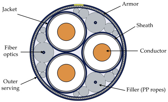
Figure 1.
Elements in a TCAC.
- The lack of radial symmetry: Customarily, an equivalent single-core ETN has been employed for the thermal current rating of TCACs [18], where the thermal resistance of the fillers must be adequately obtained. However, [18] does not take into account the filler design, hence some corrections have recently been suggested in [22,23] for larger cables;
- The location of the OF: In TCACs, it is usually embedded in the filler employed to support the armor bedding (Figure 1). This particular location is not explicitly included in any of the ETNs of TCACs reviewed by the authors. Moreover, the correlation between conductor temperature and DTS temperature is affected by the filler design (either extruded or made of PP ropes);
- Loss allocation: The ETN requires as inputs the losses in all the cable components (conductors, sheath/screen and armor). However, it is well-known that the IEC 60287 standard [18] overestimates the power losses in this type of cables. In this sense, 2D simulations based on the finite element method (FEM) were extensively employed for validating the performance of the ETN [20]. Nevertheless, both [18] and 2D-FEM models lead to important errors due to the simplifying assumptions considered, where relevant aspects regarding TCAC design are not taken into account, such as the twisting of armor wires and conductors.
Regarding the last issue, 3D-FEM simulations have proven to provide accurate results in the losses’ calculation [24,25,26], at the expense of high demanding computations. Due to recent advances [26,27,28], the length of the geometry to be simulated can be strongly reduced, achieving a saving of about 95% in terms of computation time for solving complex TCACs [28]. This improvement has made it possible to develop a fully coupled electrothermal model for simultaneously evaluating the temperature and ampacity of TCACs [29,30].
Considering all the above, this work tackles the issues observed in TCACs by proposing a new procedure for improving the accuracy of the equivalent single-core ETN for the estimation of the conductor temperature through DTS measurements, using the power of 3D-FEM simulations.
2. FEM-Based Simulation
Recent advances have helped in reducing the length, L, of TCACs 3D-FEM models by exploiting the symmetries found both in the geometry and the electromagnetic field distribution within this type of cable [26,27,28], so it is now possible to simulate a cable geometry as short as
where is the crossing pitch, N is the number of armor wires and and are, respectively, the armor wire and phase conductor lay length (twisted in opposite directions). In this situation, rotated periodicity boundary conditions can be applied, where the twisting of power cores is taken into account when mapping the source boundary into the destination boundary (Figure 2). This was done through the rotational displacement () of the power cores for a model length equal to L, defined as
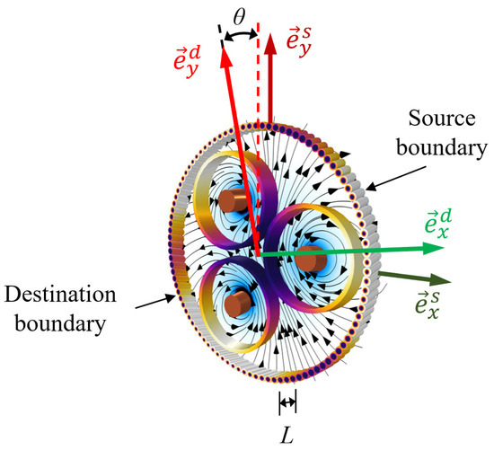
Figure 2.
Rotated periodicity in a TCAC.
Through this ultra-shortened 3D model, a reduction of approximately 95% is achieved in the computation time, taking less than 60 s to solve a complex TCAC in a laptop with 64 GB of RAM memory and a i7 processor [28].
Due to this improvement, it is now possible to develop a fully coupled electrothermal model for evaluating the temperature and ampacity of TCACs [29,30]. To this aim, a detailed 3D-FEM model is required to include the main dimensions and properties of all the elements involved in this type of cable, such as conductors, sheaths, armor wires, fillers, semiconductive screens, and fiber-optics cables. Furthermore, the accuracy of the model improves if heat transfer by radiation and natural convection inside the cable air gaps is included (as recommended in [23,31]). However, this would lead to highly demanding computations if a fully coupled 3D electrothermal FEM model is employed. To overcome this problem, Ref. [30] proposed a new fully coupled hybrid 2D-thermal/3D-electromagnetic model, where the ultra-shortened 3D electromagnetic model presented earlier is coupled with a detailed 2D thermal model. This approach is iteratively solved as follows (Figure 3): the electromagnetic losses are obtained in the periodic 3D geometry. Then, they are taken as inputs in the 2D thermal model, where the temperature distribution in all the elements of the power cable is obtained. Eventually, the temperature distribution in the metallic elements is taken as input in the 3D geometry for updating their electrical resistivity, so that electromagnetic losses can also be updated.
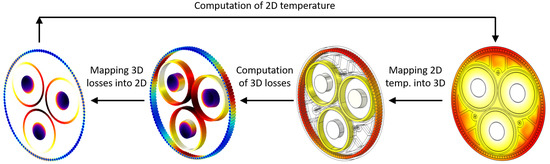
Figure 3.
Sequence for mapping magnitudes between 2D and 3D geometries.
It should be noticed that the 2D thermal problem involves the boundary conditions represented in Figure 4, where forced convection is assumed in the water-soil interface, defined by a convection heat transfer coefficient h, where is the burial depth of the cables, is the soil thermal conductivity, and is the ambient temperature. Additionally, for cables with extruded fillers, the FEM model also solves the problem of air convection inside the cable air-gaps, where surface-to-surface heat radiation is defined by the emissivity .
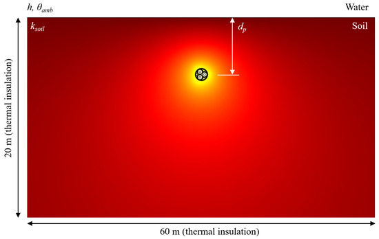
Figure 4.
Temperature distribution in TCAC and surroundings.
As can be seen, in this procedure it is required to map data between 2D and 3D geometries (Figure 3 and Figure 5). This is achieved by using a feature called “general extrusion” in the FEM software (Comsol Multiphysics [32]). This operator must be adequately configured to consider the helical path of phases and armor wires.
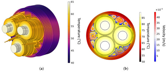
Figure 5.
(a) 3D temperature distribution; (b) temperature and air velocity fields in the 2D geometry.
Through this approach, the temperature distribution in complex TCACs is obtained in less than 4 min, all of which includes realistic boundary conditions in a detailed geometry (Figure 5).
3. Case Studies
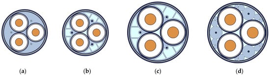
In this work, two cases were considered for analysis: a typical 132 kV, 800 mm cable and a 275 kV, 2000 mm cable with a higher voltage and larger section. Their main dimensions and parameters are summarized in Figure 6 and Table 1 and Table 2, where is the electrical resistivity, is the temperature coefficient, is the magnetic permeability, k is the thermal conductivity and C is the volumetric heat capacity. A complex permeability is employed in the armor wires to take into account hysteresis losses. Furthermore, different filler designs are considered for these cables:
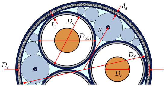
Figure 6.
Main dimensions in a TCAC.

Table 1.
Main dimensions of Cables 1 and 2 (Figure 6).
Table 2.
Main material parameters of Cables 1 and 2.
In the procedure described in the following sections, the hybrid 2D/3D electrothermal model was employed to evaluate the temperature measured by the DTS system, also providing the actual temperature of the conductor and the outer serving for the assessment. This was done for two sets of thermal boundary conditions (Case 1 and Case 2), as summarized in Table 3, characterized by different values of , and .
Table 3.
Thermal boundary conditions.
For each set of boundary conditions, Cables 1 and 2 are simulated under two different loading conditions:
- In Section 4, Section 5 and Section 6.1 the ETN is adjusted and validated for different stationary loading conditions, where fixed currents (), ranging from 50 A to (Table 1), are injected through the conductors in the FEM model.
- Alternatively, in Section 6.2, the ETN is validated for a more realistic scenario, where the per-unit () 240 h profile represented in Figure 8 is employed in the FEM model (based on data from [33]). The initial temperature in the transient studies was obtained by solving the stationary problem for a particular initial current (1 pu for Cable 1 and pu for Cable 2).
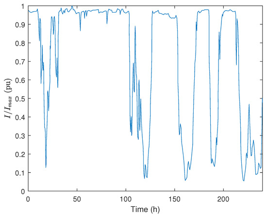 Figure 8. Normalized load profile.
4. Thermal Modeling
The main goal of this study was to obtain a static ETN specifically adjusted for a particular TCAC to estimate the conductor temperature in both stationary and dynamic loading conditions. To this aim, 3D-FEM simulations are performed to provide all the data required for the adjustment. FEM simulations will be also employed for computing the dynamic behavior of the cable temperature, providing “virtual” DTS measurements that serve as inputs for the estimation of the conductor temperature through the adjusted ETN. Thus, this section presents a description of the different stages for the derivation of the ETN proposed for TCACs. A flowchart with the different steps of the process is depicted in Figure 9.
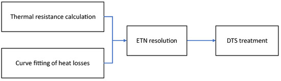
Figure 9.
Flowchart of the proposed method.
4.1. Equivalent Static Circuit
In this work, a static equivalent single-core ETN was considered for the TCAC (Figure 10), as customarily performed in [18]. This circuit is only intended for obtaining a direct relationship between DTS measurements and the conductor temperature, either under stationary or dynamic loading conditions. Thus, since it will not be employed for computing the dynamic behavior of the cable temperature, the corresponding thermal capacitances are not considered. As will be shown subsequently, this fact does not affect the accuracy of the results under dynamic loading conditions.
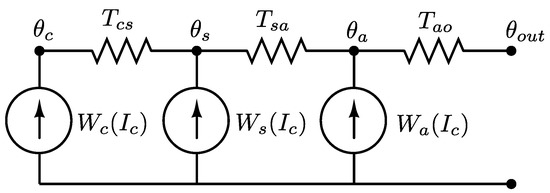
Figure 10.
Equivalent electrical circuit for the heat transfer model.
In the scheme above, , and are the heat losses in the conductor, shield, and armor, respectively, all of which depend on the conductor current, , while the corresponding temperatures are , and . The temperature of the outer surface of the cable is denoted as , and , and are the thermal resistances for each section of the cable, whose values will be obtained subsequently. It should be noticed that dielectric losses have been omitted since they are comparatively much smaller than the other losses.
4.2. Thermal Resistance Calculation
The expressions for the thermal resistances in the considered equivalent circuit are obtained from [18]. The conductor-shield resistance, , includes the contribution of all the three conductors with their corresponding insulation and semiconductor layers, yielding:
where is the thermal resistivity of the semiconductor layer and is that of the insulation layer. In the case of the shield-armor thermal resistance, , a geometric factor, G, is used as follows:
where is the thermal resistivity of the filling material and the derivation of G is provided in [18]. Finally, for the resistance , the following expression is used:
where , and are the armor bedding, outer serving and steel thermal resistivities, respectively.
4.3. Curve Fitting for Heat Losses
As commented earlier, the power losses employed as inputs in the ETN (Figure 10) are customarily derived from [18], leading to important errors in the case of TCACs. To overcome this issue, the power losses from [18] are here replaced by a simplified heat loss model, which is obtained using the information provided by FEM-based simulations for the different cables considered. The objective is to establish a numerical relation between the current in the conductor, , the temperature in different sections of the cable (conductor, shield and armor), and the corresponding heat losses. The expressions used in this study are those presented below:
where the subscripts and a stand for conductor, shield, and armor, respectively, refers to the heat losses in section j (with ), and is the corresponding temperature. The parameters with are adjusted in the least-squares sense.
For this procedure, the stationary loading conditions described in Section 3 were considered, as the results of the fitting are represented in Figure 11 for Cable 1H. In this case, the FEM-based simulation was carried out with C, with a burial depth of m and a soil thermal conductivity of W/(K · m). To evaluate the goodness of the adjustments, the corresponding coefficient of determination, , was included in each graphic. It was observed how the parabolic curve accurately matches the sample values obtained from the simulation for the three sections of the cable, with a coefficient close to 1 in all cases.
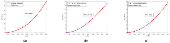
Figure 11.
Fitted heat loss curves of Cable 1H: (a) conductor; (b) shield; (c) armor (values of the coefficient of determination included).
The validity of the adjusted parameters is now assessed in order to verify whether the previously calculated values can be used for different external conditions. Furthermore, with stationary loads, the 3D-FEM simulated and curve-fitting estimated values of the heat losses for C are shown in Figure 12, where a perfect match was also obtained.
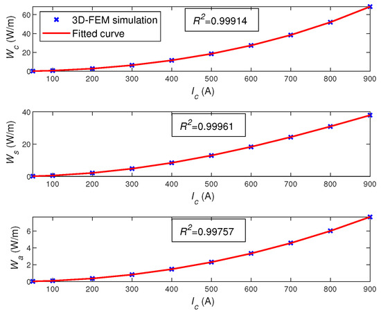
Figure 12.
Estimated and simulated heat losses for test ambient temperature C.
The good accuracy of the estimated curves was also assessed even for unrealistic external conditions (C), concluding that the FEM-based simulation can be substituted by the fitted heat loss curves (6)–(8) in the thermal model that will be presented in Section 4.4 and Section 4.5.
Similar parameters (C, m and W/(K · m)) are used for the rest of the cables (1E, 2R and 2E), obtaining the fitted curves of Figure 13.
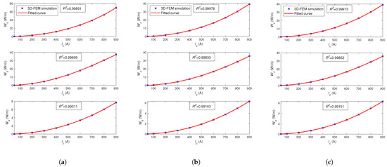
Figure 13.
Fitted curves with C, m and W/(K · m): (a) Cable 1E; (b) Cable 2R; (c) Cable 2E.
4.4. ETN Resolution
In this stage of the procedure, the circuit in Figure 10 was solved using the outer temperature, with as an input (provided by the FEM simulation), together with the Kirchhoff laws:
where , and are substituted by expressions (6)–(8) with the previously adjusted parameters, so that, for each value of the conductor current , the only unknowns are the temperatures , , and , yielding a closed system of three equations with three unknowns.
4.5. DTS Treatment
Once the temperatures , , and are calculated from the circuit resolution, the heat losses can be directly obtained from Equations (6)–(8). For the location of the DTS, the shield-armor thermal resistance, is divided into two sections, using a parameter as a DTS divider, resulting in a circuit represented in Figure 14.
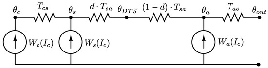
Figure 14.
Modified ETN with the DTS node.
For each value of the conductor current, , and using the temperature reading from the DTS, namely , the parameter d can be derived through the following expression:
For Cable 1H, the previously considered stationary loading conditions (with ranging from 50 A to 900 A) are introduced in the FEM software in order to simulate the measurements of , so that an estimation of the parameter d can be obtained through Equation (12), as the corresponding results are represented in Figure 15. A dependency relation of the parameter d with respect to the current can be observed, which can be adjusted using the following linear function:
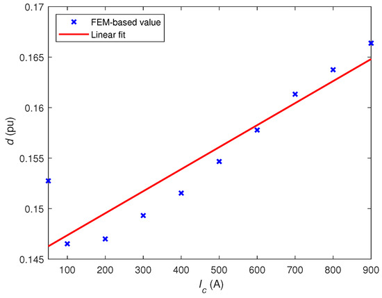
Figure 15.
Estimation results for parameter d in Cable 1H.
The mentioned adjustment was also depicted in Figure 15. The same procedure was applied to the other cables considered in this work. Figure 16 shows the estimation results for the parameter d in each case, with the corresponding linear adjustments.
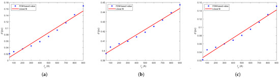
Figure 16.
Estimation results for parameter d (a) Cable 1E; (b) Cable 2R; (c) Cable 2E.
5. Estimation of the Conductor Temperature Based on DTS Measurements
Using the thermal model presented in the previous section for three-core armored submarine cables, along with the measurements of the conductor current and the temperature of the DTS, it is possible to estimate the temperature of the conductor. Once the adjustment process is completed, the substitution theorem is applied to reduce the circuit in Figure 14 to that represented in Figure 17. Using this circuit, the estimation of involves the following steps:
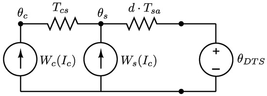
Figure 17.
Reduced electrical circuit for the calculation of .
- Step 1: The value of is introduced in Equation (13) to obtain the estimated parameter d in each case;
- Step 2: The subsequent circuit equations are considered:where the values of and are substituted by their corresponding adjusted expressions in (6) and (7);
- Step 3: The resulting system of two equations is solved to obtain :
The accuracy in the estimation of the conductor temperature is assessed in the next section for the different cables under study.
6. Numerical Validation
The performance of the proposed technique for thermal modeling and temperature estimation was tested in two different case studies. For each scenario, the results obtained for the different cables will be presented.
6.1. Base Case. Stationary Current Sweep
In the first scenario, the conductor temperature, , was estimated using the DTS information provided by the FEM software, using the stationary loading conditions described in Section 3 and considering some variations in the environmental conditions, with respect to those used for the adjustment of the proposed thermal model. For Cable 1H, the obtained results are presented in Figure 18, where the estimated values are compared to those extracted from the FEM-based simulation.
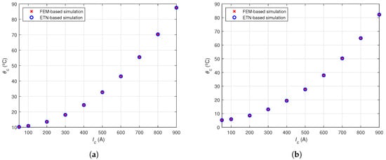
Figure 18.
Estimation results for in Cable 1H where: (a) C; (b) C.
It is observed how, in both cases, the estimations of extracted from the ETN-based model are very close to the FEM-based values for the whole range of , giving evidence of the accuracy of the proposed procedure.
Finally, in Figure 19 and Figure 20, respectively, the resulting estimations for C and C for Cables 1E, 2R and 2E are included in the base scenario ( m and W/(K · m)). In all cases, the estimation error remains under C, proving the capability of the adjusted DTS-based model to obtain an accurate estimation of the conductor temperature.
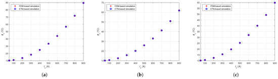
Figure 19.
Estimation results with C, m and W/(K · m) for: (a) Cable 1E; (b) Cable 2R; (c) Cable 2E.
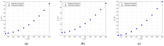
Figure 20.
Estimation results with C, m and W/(K · m) for: (a) Cable 1E; (b) Cable 2R; (c) Cable 2E.
6.2. Actual Current Profiles
In this second case, the current dynamic profile presented in Figure 8 was considered for the FEM-based simulation of a more realistic operating scenario. With this profile, different external conditions were considered for the simulations, from which the temperature was acquired and used to estimate the conductor temperature with the adjusted thermal model. The variables in this scenario are:
- Ambient temperature, ;
- Burial depth, , of the cable;
- Soil thermal conductivity, ;
- Initial conductor current with respect to the rated value, .
The values of these boundary conditions for each case were presented in Table 3. The estimation results obtained in each case are represented in Figure 21, Figure 22, Figure 23 and Figure 24 for Cables 1H, 1E, 2R, and 2E, respectively. The measurements are supposed to be taken every 9 minutes and the DTS temperature has also been represented as a reference value.
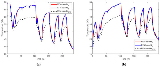
Figure 21.
Estimation results for in Cable 1H: (a) Case 1; (b) Case 2.
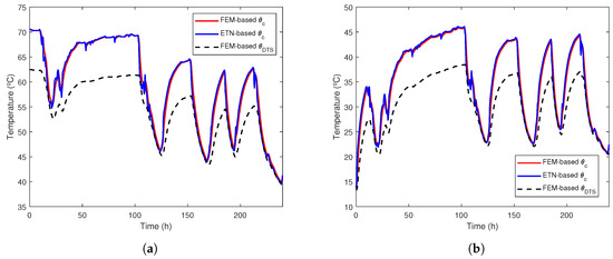
Figure 22.
Estimation results for in Cable 1E: (a) Case 1; (b) Case 2.
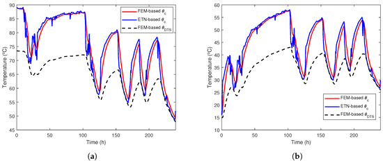
Figure 23.
Estimation results for in Cable 2R: (a) Case 1; (b) Case 2.
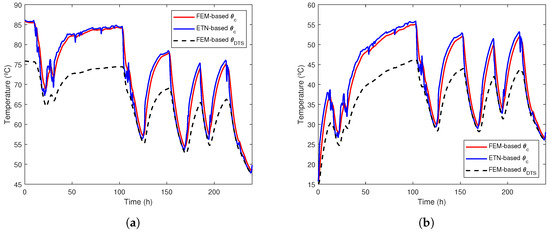
Figure 24.
Estimation results for in Cable 2E: (a) Case 1; (b) Case 2.
In these figures, it can be observed that:
Additionally, the mean relative error (MRE) and the maximum absolute error (MAE), defined as
are considered to evaluate the overall performance of the estimation. In Equation (17), N is the number of available readings and and are the ith temperature value obtained with FEM and ETN, respectively. Table 4 summarizes the MREs and MAEs for the different cables and case studies.
Table 4.
Errors obtained from the application of the ETN-based model to the 4 cables.
For the whole set of external conditions, the MREs remain under , proving that the proposed model effectively estimates the temperature of the conductor in TCACs. For the most unfavorable cases (Cables 2R and 2E), values of the MAE near C are noticed. However, although these values could be perceived as high, they correspond to quite limited periods of time, given the fact that the MRE is much lower. Moreover, the purpose of the proposed procedure is to establish, with a static thermal model, an estimation of the conductor temperature which can be used to evaluate the actual state of the cable rather than the typical option of directly using the temperature provided by the DTS [33]. In this regard, it can be concluded from Figure 23 and Figure 24 that the ETN-based (blue line) is much closer to the actual value (red line) of the temperature than (black dashed line), which is evidence of the good performance of the proposed technique. Using the typical assumption , there would be an underestimation of the temperature in most cases, which might lead to a reduction in the useful life of the TCAC, with the corresponding economic consequences [6].
Finally, an important aspect to consider is that the location of the DTS simulated in FEM might differ from the actual location of the sensor due to, for example, the tolerances in the production process. To assess the impact of this deviation in the estimation of , two additional simulations were performed for Cable 1H, changing the position of the DTS, , in , with respect to that employed in the adjustment simulation. The obtained estimations are depicted in Figure 25.
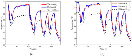
Figure 25.
Estimation results with deviations in the sensor position: (a) ; (b) .
In both cases, the estimation error has slightly increased with respect to that in Figure 21a. In order to quantify the deterioration of the results with the deviation of the sensor position, Table 5 presents the MAEs obtained in different cases.
Table 5.
MAEs obtained for different deviations in the sensor position.
In light of this table, it can be noticed that, as expected, the MAE increases with the deviation in the sensor position. However, even with this error, the estimation given by the proposed method is still valid to provide information related to the thermal state of the TCAC.
7. Conclusions
In this paper, a thermal model is proposed for three-core armored submarine cables using DTS. For each cable studied, a set of FEM-based simulations are considered, from which a simplified heat loss model is derived with a curve-fitting technique. Once the thermal resistances are calculated for each section of the cable, a parameter d, depending on the load, is also adjusted with the simulation data, representing the location of the DTS in the equivalent static circuit modeled and isolating a portion of the cable from the outside.
An error assessment study was also made to conclude that for reasonable deviations in the position of the sensor with respect to the simulated location, the estimation does not deteriorate substantially. Two different scenarios were considered to test the performance of the adjusted thermal model:
- With a stationary current sweep, the proposed thermal model accurately estimates the conductor temperature for changing values of the ambient temperature.
- For a more realistic current profile and pronounced deviations in the external conditions, the obtained MREs range from 1.11% for Cable 1H to % for Cable 2E. In absolute terms, the maximum deviation of the estimated temperature with respect to the simulated value is C for Cable 1H, and C in the most unfavorable case (Cable 2R).
The proposed thermal model allows, as mentioned before, to establish a more accurate evaluation of the state of the submarine cable in terms of the temperature of the conductor for a certain current, which can be used in some dynamic line rating applications. The adjusted cable parameters of the model can be obtained by the corresponding manufacturer or by the utilities, using the procedure described in this paper with FEM-based simulations. It must be noticed that this adjustment only depends on the conductor current, being unaffected by other environmental boundary conditions, so it can be easily integrated into existing RTTR.
Further research might be oriented to enhance the equivalent model, including some dynamic effects in order to improve the estimation of the temperature under sudden variations in the current.
Author Contributions
Conceptualization, M.Á.G.-C., J.C.d.-P.-L., A.B.-S., P.C.-R. and J.A.R.-M.; methodology, M.Á.G.-C., J.C.d.-P.-L., A.B.-S., P.C.-R. and J.A.R.-M.; software, M.Á.G.-C. and J.C.d.-P.-L.; validation, M.Á.G.-C., J.C.d.-P.-L., A.B.-S., P.C.-R. and J.A.R.-M.; formal analysis, M.Á.G.-C., J.C.d.-P.-L., A.B.-S., P.C.-R. and J.A.R.-M.; investigation, M.Á.G.-C., J.C.d.-P.-L., A.B.-S., P.C.-R. and J.A.R.-M.; data curation, M.Á.G.-C. and J.C.d.-P.-L.; writing—original draft preparation, M.Á.G.-C. and J.C.d.-P.-L.; writing—review and editing, M.Á.G.-C., J.C.d.-P.-L., A.B.-S., P.C.-R. and J.A.R.-M. All authors have read and agreed to the published version of the manuscript.
Funding
This research was funded by FEDER/Ministerio de Ciencia e Innovación—Agencia Estatal de Investigación under the project ENE2017-89669-R and by the Universidad de Sevilla (VI PPIT-US) under grant 2018/00000740.
Institutional Review Board Statement
Not applicable.
Informed Consent Statement
Not applicable.
Data Availability Statement
Not applicable.
Conflicts of Interest
The authors declare no conflict of interest.
Abbreviations
The following abbreviations are used in this manuscript:
| DTS | Distributed Temperature Sensing |
| IEC | International Electrotechnical Commission |
| ETN | Equivalent Thermal Network |
| FEM | Finite Element Method |
| MAE | Maximum Absolute Error |
| MRE | Mean Relative Error |
| OF | Optical Fiber |
| OWPP | Offshore Wind Power Plants |
| PE | Polyethylene |
| PP | Polypropylene |
| RTTR | Real-Time Thermal Rating |
| TCAC | Three-Core Armored Cable |
| XLPE | Cross-Linked Polyethylene |
References
- Wind Europe. Wind Energy in Europe: Outlook to 2023. Available online: https://windeurope.org/about-wind/reports/wind-energy-in-europe-outlook-to-2023/ (accessed on 16 May 2021).
- CIGRE Working Group B1.47. TB 680-Implementation of Long AC HV and EHV Cable Systems; CIGRE: Paris, France, 2017. [Google Scholar]
- Nielsen, J.; Olsen, R. Large scale monitoring of extruded cables—Review of TSOs needs and options. In Proceedings of the 10th International Conference on Insulated Power Cables, Versailles, France, 23–27 June 2019. [Google Scholar]
- CIGRE Working Group B1.40. TB 610—Offshore Generation Cable Connections; CIGRE: Paris, France, 2015. [Google Scholar]
- Leemans, P.; Mampaey, B.; Martin, P.; Cromboom, D.; Falkenback, J.P. Belgian experience with real time thermal rating system in combination with distributed temperature sensing techniques. In Proceedings of the 9th International Conference on Insulated Power Cables, Versailles, France, 21–25 June 2015. [Google Scholar]
- Worzyk, T. Submarine Power Cables. Design, Installation, Repair, Environmental Aspects; Springer: Berlin, Germany, 2009; ISBN 978-3-642-01269-3. [Google Scholar]
- CIGRE Working Group B1.57. TB 815—Update of Service Experience of HV Underground and Submarine Cable Systems; CIGRE: Paris, France, 2020. [Google Scholar]
- CIGRE Working Group B1.52. TB 773—Fault Location on Land and Submarine Links (AC & DC); CIGRE: Paris, France, 2019. [Google Scholar]
- CIGRE Working Group B1.45. TB 756—Thermal Monitoring of Cable Circuits and Grid Operators’ Use of Dynamic Rating Systems; CIGRE: Paris, France, 2019. [Google Scholar]
- Kazerooni, A.; Scott, C.; Ruthven, D.; Peat, W.; Hessel, E. Technical recommendations for implementation of dynamic cable rating system—cable modelling. In Proceedings of the 25th International Conference on Electricity Distribution (CIRED), Madrid, Spain, 3–6 June 2019. [Google Scholar]
- Aegerter, D.; Meier, S. Model-based predictive control for use in RTTR temperature sensing systems of high voltage cables. In Proceedings of the 10th International Conference on Insulated Power Cables, Versailles, France, 23–27 June 2019. [Google Scholar]
- Chen, Y.; Wang, S.; Hao, Y.; Yao, K.; Li, H.; Jia, F.; Shi, Q.; Yue, D.; Cheng, Y. The 500 kV Oil-filled Submarine Cable Temperature Monitoring System Based on BOTDA Distributed Optical Fiber Sensing Technology. In Proceedings of the International Conference on Sensing, Measurement and Data Analytics in the Era of Artificial Intelligence, Xi’an, China, 15–17 October 2020. [Google Scholar] [CrossRef]
- Callender, G.; Ellis, D.J.; Goddard, K.F.; Dix, J.K.; Pilgrim, J.A. Low Computational Cost Model for Convective Heat Transfer from Submarine Cables. IEEE Trans. Power Deliv. 2020, 36, 760–768. [Google Scholar] [CrossRef]
- Lux, J.; Olschewski, M.; Schäfer, P.; Hill, W. Real-Time Determination of Depth of Burial Profiles for Submarine Power Cables. IEEE Trans. Power Deliv. 2019, 34, 1079–1086. [Google Scholar] [CrossRef]
- Van Oosterom, J.; Van Doeland, W.; Koning, R. Experiences with depth of burial monitoring in the North Sea using Distributed Temperature Sensing. In Proceedings of the 10th International Conference on Insulated Power Cables, Versailles, France, 23–27 June 2019. [Google Scholar]
- CIGRE Working Group B1.35. TB 640—A Guide for Rating Calculations of Insulated Cables; CIGRE: Paris, France, 2015. [Google Scholar]
- Watanabe, T.; Muramatsu, Y.; Nakanishi, M. Operating records and recent technology of DTS systems and dynamic rating systems (DRS). In Proceedings of the 9th International Conference on Insulated Power Cables, Versailles, France, 21–25 June 2015. [Google Scholar]
- IEC. 60287-1-1 Electric Cables–Calculation of the Current Rating–Part 1-1: Current Rating Equations (100% Load Factor) and Calculation of Losses–General; IEC: Geneva, Switzerland, 2015. [Google Scholar]
- Nielsen, T.V.M.; Jakobsen, S.; Savaghebi, M. Dynamic Rating of Three-Core XLPE Submarine Cables for Offshore Wind Farms. Appl. Sci. 2019, 9, 800. [Google Scholar] [CrossRef] [Green Version]
- Nielsen, T.V.M.; Jakobsen, S.; Savaghebi, M. Dynamic rating of three-core XLPE submarine cables considering the impact of renewable power generation. In Proceedings of the IEEE 13th International Conference on Compatibility, Power Electronics and Power Engineering, Sonderborg, Denmark, 23–25 April 2019. [Google Scholar] [CrossRef]
- Enescu, D.; Russo, A.; Porumb, R.; Seritan, G. Dynamic thermal rating of electric cables: A conceptual overview. In Proceedings of the 55th International Universities Power Engineering Conference, Turin, Italy, 1–4 September 2020. [Google Scholar] [CrossRef]
- Zhan, Q.; Rhuan, J.; Tang, K.; Tang, L.; Liu, Y.; Li, H.; Ou, X. Real-time calculation of three core cable conductor temperature based on thermal circuit model with thermal resistance correction. J. Eng. 2019, 16, 2036–2041. [Google Scholar] [CrossRef]
- Chatzipetros, D.; Pilgrim, J.A. Review of the Accuracy of Single Core Equivalent Thermal Model for Offshore Wind Farm Cables. IEEE Trans. Power Deliv. 2018, 33, 1913–1921. [Google Scholar] [CrossRef] [Green Version]
- Benato, R.; Dambone Sessa, S.; Forzan, M.; Marelli, M.; Pietribiasi, D. Core laying pitch-long 3D finite element model of an AC three-core armoured submarine cable with a length of 3 metres. Electr. Power Syst. Res. 2017, 150, 137–143. [Google Scholar] [CrossRef]
- Sturm, S.; Kütchler, A.; Paulus, J.; Stølan, R.; Berger, F. 3D-FEM modelling of losses in armoured submarine power cables and comparison with meassurements. In Proceedings of the CIGRÉ Session, Paris, France, 24 August–3 September 2020. [Google Scholar]
- del-Pino-López, J.C.; Hatlo, M.; Cruz-Romero, P. On simplified 3D finite element simulations of three-core armored power cables. Energies 2018, 11, 3081. [Google Scholar] [CrossRef] [Green Version]
- del-Pino-López, J.C.; Cruz-Romero, P.; Sánchez-Díaz, L.C. Loss allocation in submarine armored three-core HVAC power cables. In Proceedings of the 2020 IEEE International Conference on Enviroment and Electrical Enginnering and 2020 IEEE Industrial and Comercial Power Systems Europe (EEEIC/I and CPS Europe), Madrid, Spain, 9–12 June 2020. [Google Scholar] [CrossRef]
- del-Pino-López, J.C.; Cruz-Romero, P. Use of 3D-FEM tools to improve loss allocation in three-core armored cables. Energies 2021, 14, 2434. [Google Scholar] [CrossRef]
- del-Pino-López, J.C.; Cruz-Romero, P. A 3D parametric thermal analysis of submarine three-core power cables. In Proceedings of the Renewable Energy and Power Quality Journal (ICREPQ’20), Granada, Spain, 2–4 September 2020. [Google Scholar]
- del-Pino-López, J.C.; Cruz-Romero, P. Hybrid 2D/3D fully coupled electrothermal model for three-core submarine armored cables. In Proceedings of the Comsol Conference Europe, Online, 14–15 October 2020; Available online: https://www.comsol.com/paper/hybrid-2d-3d-fully-coupled-electrothermal-model-for-three-core-submarine-armored-95651 (accessed on 16 May 2021).
- De Wild, F.; Anders, G.J.; Kamara, W.; Canada, C. Overview of CIGRÉ WG B1.56 regarding the verification of cable current ratings. In Proceedings of the 10th International Conference on Insulated Power Cables, Versailles, France, 23–27 June 2019. [Google Scholar]
- COMSOL Multiphysics®v.5.6. COMSOL AB: Stockholm, Sweden. Available online: http://www.comsol.com (accessed on 30 March 2021).
- Sarto, T.; Holbøll, J.; Arana, I.; Olsen, R.A. Thermo-electric equivalent of submarine export cable system in wind farms—Model development and validation. In Proceedings of the CIGRÉ Session, Paris, France, 26–31 August 2018. [Google Scholar]
Publisher’s Note: MDPI stays neutral with regard to jurisdictional claims in published maps and institutional affiliations. |
© 2021 by the authors. Licensee MDPI, Basel, Switzerland. This article is an open access article distributed under the terms and conditions of the Creative Commons Attribution (CC BY) license (https://creativecommons.org/licenses/by/4.0/).