Article

An Improved Method of Reservoir Facies Modeling Based on Generative Adversarial Networks

1
The Key Laboratory of Orogenic Belts and Crustal Evolution, School of Earth and Space Sciences, Peking University, Beijing 100871, China
2
Research Institute of Petroleum Exploration & Development, PetroChina, Beijing 100083, China
*
Author to whom correspondence should be addressed.
Energies 2021, 14(13), 3873; https://doi.org/10.3390/en14133873
Submission received: 8 May 2021 / Revised: 10 June 2021 / Accepted: 22 June 2021 / Published: 28 June 2021

Abstract

:
As the reservoir and its attribute distribution are obviously controlled by sedimentary facies, the facies modeling is one of the important bases for delineating the area of high-quality reservoir and characterizing the attribute parameter distribution. There are a large number of continental sedimentary reservoirs with strong heterogeneity in China, the geometry and distribution of various sedimentary microfacies are relatively complex. The traditional geostatistics methods which have shortage in characterization of the complex and non-stationary geological patterns, have limitation in facies modeling of continental sedimentary reservoirs. The generative adversarial network (GANs) is a recent state-of-the-art deep learning method, which has capabilities of pattern learning and generation, and is widely used in the domain of image generation. Because of the similarity in content and structure between facies models and specific images (such as fluvial facies and the images of modern rivers), and the various images generated by GANs are often more complex than reservoir facies models, GANs has potential to be used in reservoir facies modeling. Therefore, this paper proposes a reservoir facies modeling method based on GANs: (1) for unconditional modeling, select training images (TIs) based on priori geological knowledge, and use GANs to learn priori geological patterns in TIs, then generate the reservoir facies model by GANs; (2) for conditional modeling, a training method of “unconditional-conditional simulation cooperation” (UCSC) is used to realize the constraint of hard data while learning the priori geological patterns. Testing the method using both synthetic data and actual data from oil field, the results meet perfectly the priori geological patterns and honor the well point hard data, and show that this method can overcome the limitation that traditional geostatistics are difficult to deal with the complex non-stationary patterns and improve the conditional constraint effect of GANs based methods. Given its good performance in facies modeling, the method has a good prospect in practical application.

1. Introduction

Reservoir modeling which is the fine quantitative description of the spatial distribution characteristics and the variation trends of reservoir and its attribute parameters, is an important basis for reservoir evaluation, numerical simulation and development management [1]. At the oilfield scale, sedimentary microfacies plays an important role in controlling the spatial distribution of reservoir and its attributes. High quality reservoirs are often distributed in one or several types of sedimentary microfacies [2,3], and the distribution of various attribute parameters among different sedimentary microfacies presents different trends [4]. It is of great significance to establish reservoir facies model as one of the important contents and key steps of reservoir modeling.
Geostatistics is one of the most commonly used reservoir facies modeling methods. After decades of development, a series of mature methods, such as two-point geostatistics [5,6] and multi-point geostatistics [7,8,9], have been formed. However, it is difficult for traditional geostatistics methods to produce complex and non-stationary geological bodies. Two-point geostatistics uses the variogram to represent the spatial variability, but the variogram can only characterize the correlation between the two points in space. The spatial structure with different morphology and distribution characteristics may produce similar variograms (Figure 1), which makes it difficult to characterize, distinguish and reproduce the geometry of complex objects [10]. Multi-point geostatistics replace variogram by the spatial multi-point relationship represented by training images (TIs), and can better duel with the continuous structures such as rivers [7,8,9], but the modeling effect depends on the stationarity of the problem. The effects are poor when the non-stationary problem is encountered (Figure 2) [11]. There are many continental sedimentary reservoirs with strong heterogeneity in China, and the geometry and distribution of various sedimentary microfacies are relatively complex [12], which means that strong non-stationarity is often encountered, and cause the great limitations of traditional methods in practice.
The generative adversarial networks (GANs) is a recent state-of-the-art deep learning method [13] which has capabilities of pattern learning and generation, and is widely used in the field of image generation (Figure 3a) [13,14]. Reservoir facies models are similar to specific images in content and data structure, such as images of modern river channel and corresponding models of anastomosing river channel (Figure 3b,c). Additionally, many kinds of images which are more complex than reservoir facies models, such as faces and scenes (Figure 3a), are non-stationary from the perspective of facies modeling. Thus, the powerful capabilities and successful applications in image generation make GANs have the potential to characterize complex and non-stationary geological bodies in reservoir facies modeling, and with a good application prospect.
The earlier application of neural network method to reservoir facies modeling can be traced back to the 1990s. Caers (1998) used two-layer feedforward neural network to learn geological patterns in TIs and reproduced the facies models [15]. However, the realizations are not stable and the training is difficult due to the limitations of network depth and optimization method, so the related researches have not been extensively applied [16]. In recent years, with the maturity and popularization of deep learning, neural networks re-gained attention in reservoir facies modeling [17,18,19,20,21,22], among which the research based on GANs have achieved good results [17,18,19,20]. Chan et al. (2017) realized the reproduction of meandering river with various curvatures by using GANs [17]; Laloy et al. (2018) combined Markov Monte Carlo method with the GANs, and realized the simulation of multiple sedimentary microfacies [18]. However, Chan et al. (2017) and Laloy et al. (2018) only discussed the generation of geological patterns, without considering the well point data which constrain the distribution of sedimentary microfacies. DuPont et al. (2018) [19] and Zhang et al. (2019) [20] of Schlumberger proposed a conditional modeling method (hereinafter referred to as “D-Z method”) by improving the training process of GANs, that the results can be honor to both prior geological patterns and well point constraints. However, this method still has the following shortcomings: (1) the results of conditional simulation are not stable, and constrain effect of well point data is not very good; (2) the non-stationary model established is relatively simple, and it is only verified on the synthetic data without the application in the actual oilfield data; (3) modeling successfully using GANs is with many tricks, and evidently depending on the implementation details of method, but the reports from commercial software organizations are lack of relevant details.
Therefore, this paper proposes an improved facies modeling method based on GANs (using “UCSC” method in conditional modeling) which: (1) overcomes the limitation of traditional geostatistics [5,6,7,8,9] with good capability to reproduce the complex non-stationary patterns in reservoir modeling; (2) goes further some of current GANs based methods [17,18] in considering the hard data constrains to the distribution of sedimentary microfacies; (3) improves and realizes better hard data constrains effect than D-Z method [19,20]. Furthermore, this paper also establishes a facies modeling workflow based on proposed method to provide the good practicability and suitability, and tests proposed method in actual oil field data of continental reservoir.

2. Principle of Method

GANs is a kind of differentiable generative model. The model is composed of two competing networks based on game theory scene [13] (Figure 4): generator network (G) generates images from random noises (vector form) corresponding to certain distribution; discriminator network (D) is responsible for distinguishing TIs which represent real images from images generated by generator network. The two networks are optimized against each other, through training: the generator network improves its generation capability to make the generated images and the TIs as similar as possible, so that the discriminator network is difficult to distinguish whether the images are generated by the generator network; the discriminator network improves its discrimination capability to distinguish the TIs and the images generated by the generator network as much as possible. The training continues until the similarity between the generated images and the TIs is high and the discriminator network cannot distinguish TIs from generated images effectively.
The objective function is shown in Formula (1): G represents the generator network, D represents the discriminator network, x represents the TIs, z represents the random noises, G(z) is the generated images, D(x) is the probability of discriminator network judging whether the TIs are real, D(G(z)) is the probability of judging whether the generated images are real. V(D,G) represents the synthetic loss of these two networks which are adversarial: the training of generator network makes the generated images more realistic, which means D(G(z)) is as large as possible and V(D,G) is as small as possible (as shown by min G ); the training of discriminator network enhance the discrimination capability, which means 1-D(G(z)), D(x) are as large as possible and V(D,G) is as large as possible (as shown by max D ).
min G max D V D , G = Ε x ~ P data log D x + Ε z ~ P m o d e l log 1 D G z
In practice, the generator network and the discriminator network are trained alternately, as shown in Figure 4. When training the discriminator network (process ①), the loss function is the cross entropy between the discrimination results of the TIs and the generated images and the labels of true and false (labels for TIs are true and labels for generated image are false). The error back-propagates in the discriminator network, and the parameters of the discriminator network are optimized. When training the generator network (process ②), the loss function is the cross entropy function between the discrimination results and the labels of true. The error transfers to the generator network through the discriminator network without optimizing its parameters, then back-propagates in generator network to optimize generator network’s parameters.
In the GANs model initially proposed by Goodfellow (2014), both the generator network and the discriminator network are deep feedforward networks [13]. The training process is unstable and the generated images have certain distortions. To solve these problems, Radford (2015) proposed deep convolution generative adversarial networks (DCGANs) using deconvolution neural networks and convolution neural networks as generator networks and discriminator networks, respectively (Figure 5). By using the powerful feature extraction capability of convolutional neural networks for images, the stability of training and the quality of generated images are effectively improved. In this paper, the proposed UCSC method is based on DCGANs.

3. Facies Modeling Methods

3.1. Concept

Multi-point geostatistics classifies facies modeling into unconditional simulation and conditional simulation according to whether there are hard data constraints in the modeling process. Both of them learn the prior geological patterns in the modeling process. The difference is that the conditional simulation integrates hard data constraints, while the unconditional simulation modeling does not consider the hard data constraints. These concepts continue to use in facies modeling based on GANs.
Based on a priori geological pattern, unconditional modeling can provide a large number of different realizations for various complex modeling objects, or provide new TIs for multi-point geostatistics and other methods. In many application scenarios, conditional modeling is also needed to make the facies models meet both the prior geological patterns and the hard data, so as to characterize the morphology and distribution of sedimentary microfacies more accurately.

3.2. Unconditional Modeling Method

The method to realize unconditional modeling by generative adversarial network is similar to the common image generation method. The TIs are used to provide priori geological patterns, and generator network is trained adversarial with discriminator network to learn these patterns and gains the capability to generate facies models which meet these patterns. The basic steps are as follows (Figure 6):
(1)
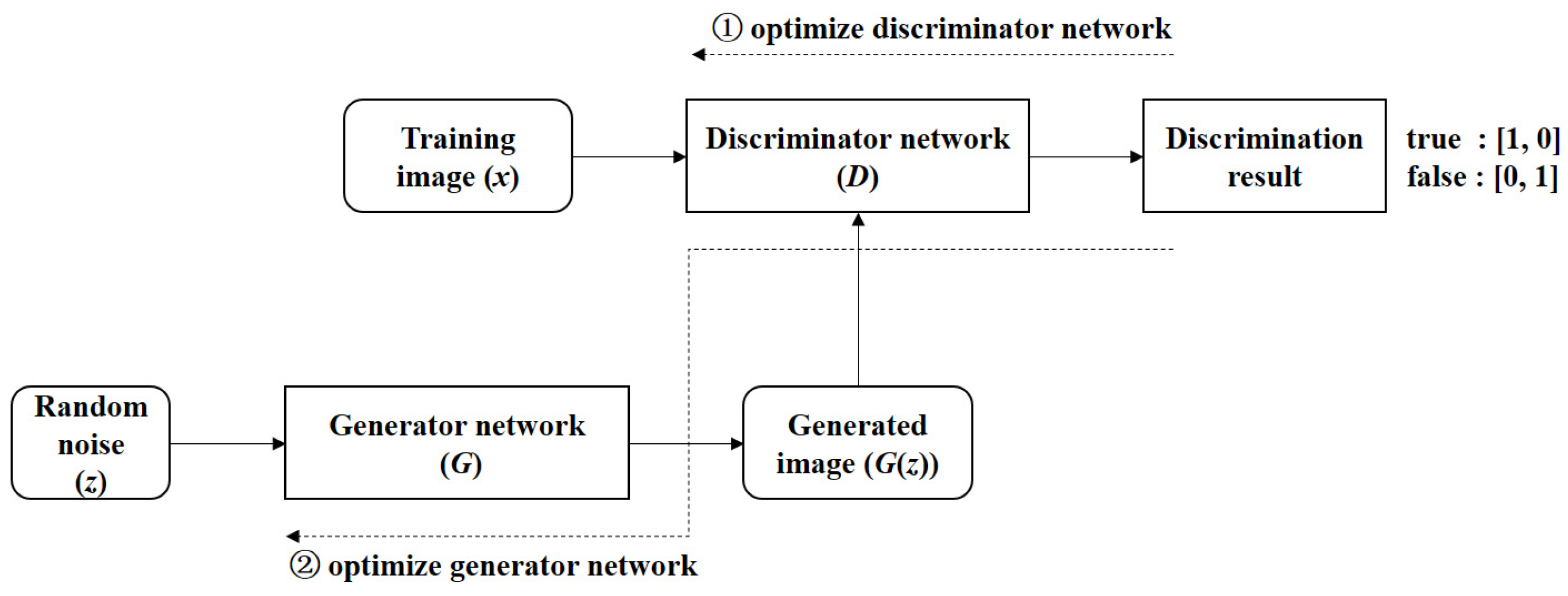
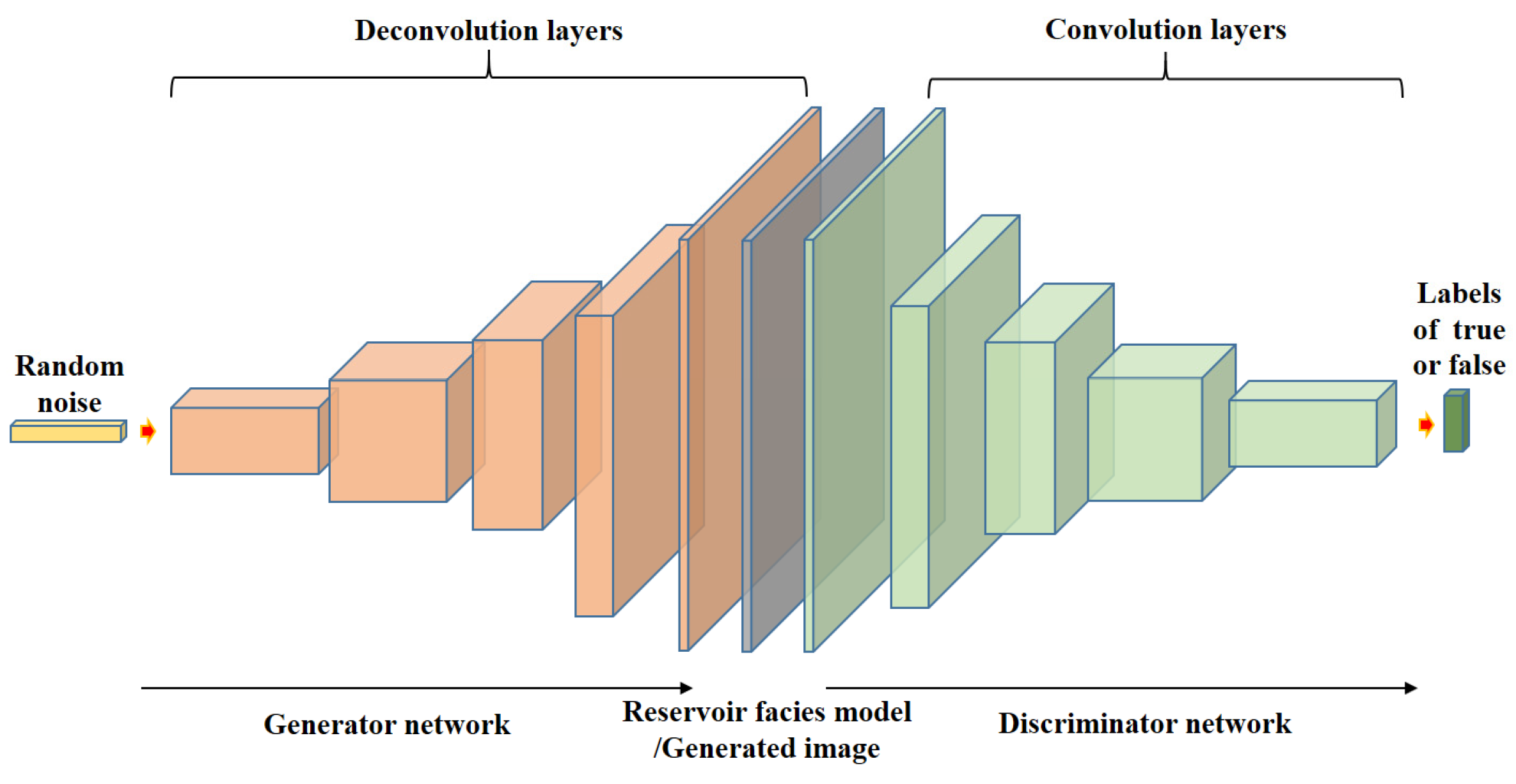
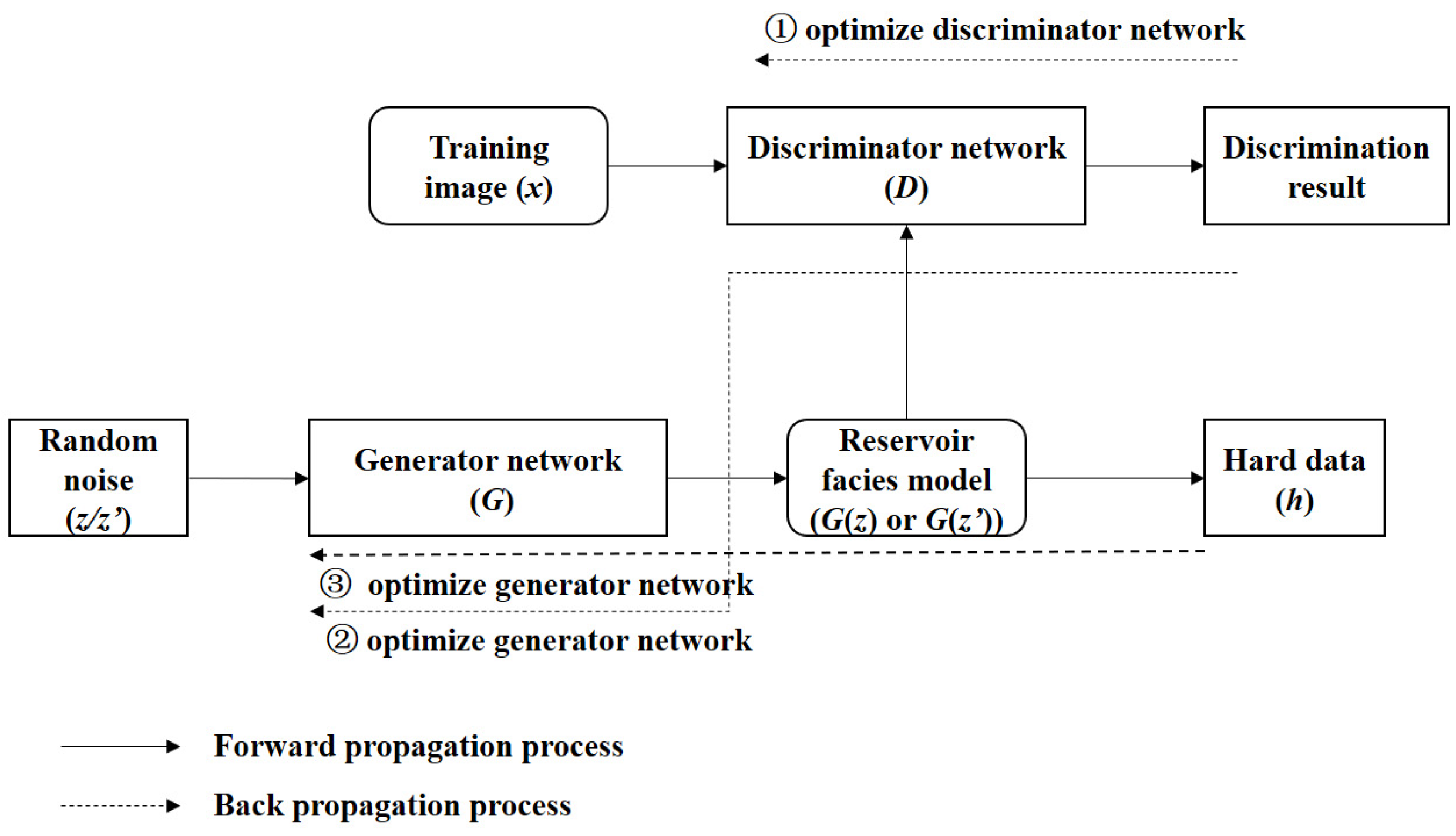
The cross entropy of the discrimination results of TIs x and generated facies models G(z) with labels of true and false is propagated back in discriminator network D, and its parameters are updated to enhance its discrimination capability (Figure 6, process ①).
(2)
The cross entropy of the discrimination results of generated facies models G(z) with the true labels is propagated back in generator network G, and its parameters are updated to enhance its capability of generating the facies models which meet the prior geological patterns (Figure 6, process ②).
(3)
Step 1 and step 2 are carried out alternately according to a certain frequency in an epoch, until the generator network is able to generate facies models consistent with the prior geological patterns.

3.3. Conditional Modeling Method

The key to realize conditional modeling by using GANs is to make the distribution of sedimentary microfacies honor to the constraints of hard data on the basis of learning the prior geological patterns. In the D-Z method, the generator network and discriminator network are trained first, and then the random noises z are adjusted according to the hard data constraints [19,20]. However, the adjustment of random noises z is not enough to realize the hard data constraints perfectly resulting in poor modeling effect. Therefore, to meet the high requirements of hard data constraints in some application scenario, such as reservoir facies modeling of oilfield, a training method of running unconditional simulation and conditional simulation simultaneously for a certain number of random noises z’, that we call “unconditional-conditional simulation cooperation” (UCSC) method, is proposed in this paper. This method optimizes generator network’s parameters directly instead of the adjusting random noises to realize a larger adjustment for honoring hard data perfectly in the conditional modeling results. The implementation steps are as follows:
(1)
Taking random noises z and TIs x as input, the generator network G and discriminator network D (Figure 6, processes ① and ②) are alternately trained. The process is the same as step 1 and step 2 in the unconditional modeling method.
(2)
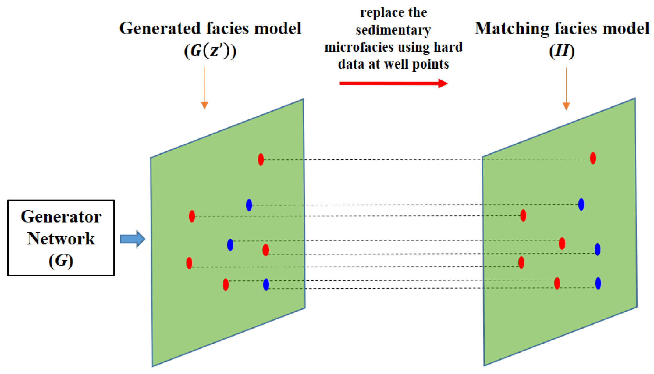
Taking random noises z’ as input, the facies models G(z’) are generated, then the error between the G(z’) and hard data h at the well point is calculated. The generator network G is updated by back propagating the error and tries to generate facies models honoring the hard data h (Figure 6, process ③).
(3)
Step 1 and step 2 are carried out alternately until the generated facies models meet the prior geological patterns.
(4)
Input the random noises z’ into the generator network G to generate the modeling results G(z’).

3.4. Loss Function

Loss function is the goal of optimization. Facies modeling based on GANs requires that the facies models generated by generator network have the same geological patterns as the TIs, and can be consistent with the hard data on well points, and the discriminator network should have the capability to distinguish the TIs from the generated models. Therefore, it is necessary to design and implement different loss functions for different objectives which can be divided into two types: pattern loss function for learning the geological patterns and conditional loss function for realizing hard data constraints.
The discriminator network takes the pattern loss function as the objective to enhance the discrimination capability (Figure 6, process ①). The function consists of two parts (Formula (2)), Lossreal-real represents the cross entropy between the discrimination results of the TIs and the labels of true, Lossfake-fake represents the cross entropy between the discrimination results of the generated facies models and the labels of false. The smaller the Losspattern, the stronger the discrimination capability. Formula (3) is the cross entropy function, where y represents the labels and y ^ represents the discrimination results.
Loss p a t t e r n = Loss r e a l r e a l + Loss f a k e f a k e
Loss = L y , y ^ = y log y ^ 1 y log 1 y ^
The generator network takes the pattern loss function as the objective to optimize the pattern generation capability (Figure 6, process ②), and takes the conditional loss function as the objective to realize the hard data constraints (Figure 6, process ③;). The pattern loss function which characterizes the similarity between the generated facies models and the TIs is the cross entropy of the discrimination results of the generated facies models and the labels of true (Formula (4)). That is, the generator network is optimized in the direction that the discriminator network judges the generated facies models as true. The conditional loss function is used to measure the matching between the generated facies models and the hard data at well point, by calculating the N-norm distance between them (Formula (5)). 1-norm or 2-norm is usually selected, G(z’) represents the generated facies models, h represents the hard data. The value of α is adjusted to maintaining the effective constraints of hard data to sedimentary microfacies distribution. A higher α gives stronger constraints by back propagating the larger conditional loss, but affects the effect of pattern reproduction by the stronger tuning of sedimentary microfacies distribution to honor the hard data. Generally, the setting of α should balance these two aspects.
Loss p a t t e r n = Loss f a k e r e a l
Loss c o n d i t i o n a l = L y , G z = α G z h n   α 1
A way to realize the conditional loss function is to use the hard data of well points to replace the sedimentary microfacies in the generated facies models to form the matching facies models, and then calculate the loss function between the corresponding positions of the two models (as shown in Figure 7). The method does not need additional matrix to extract the sedimentary microfacies at well points from generated facies models to calculate the loss function, which avoids the gradient vanishing caused by a sparse matrix.

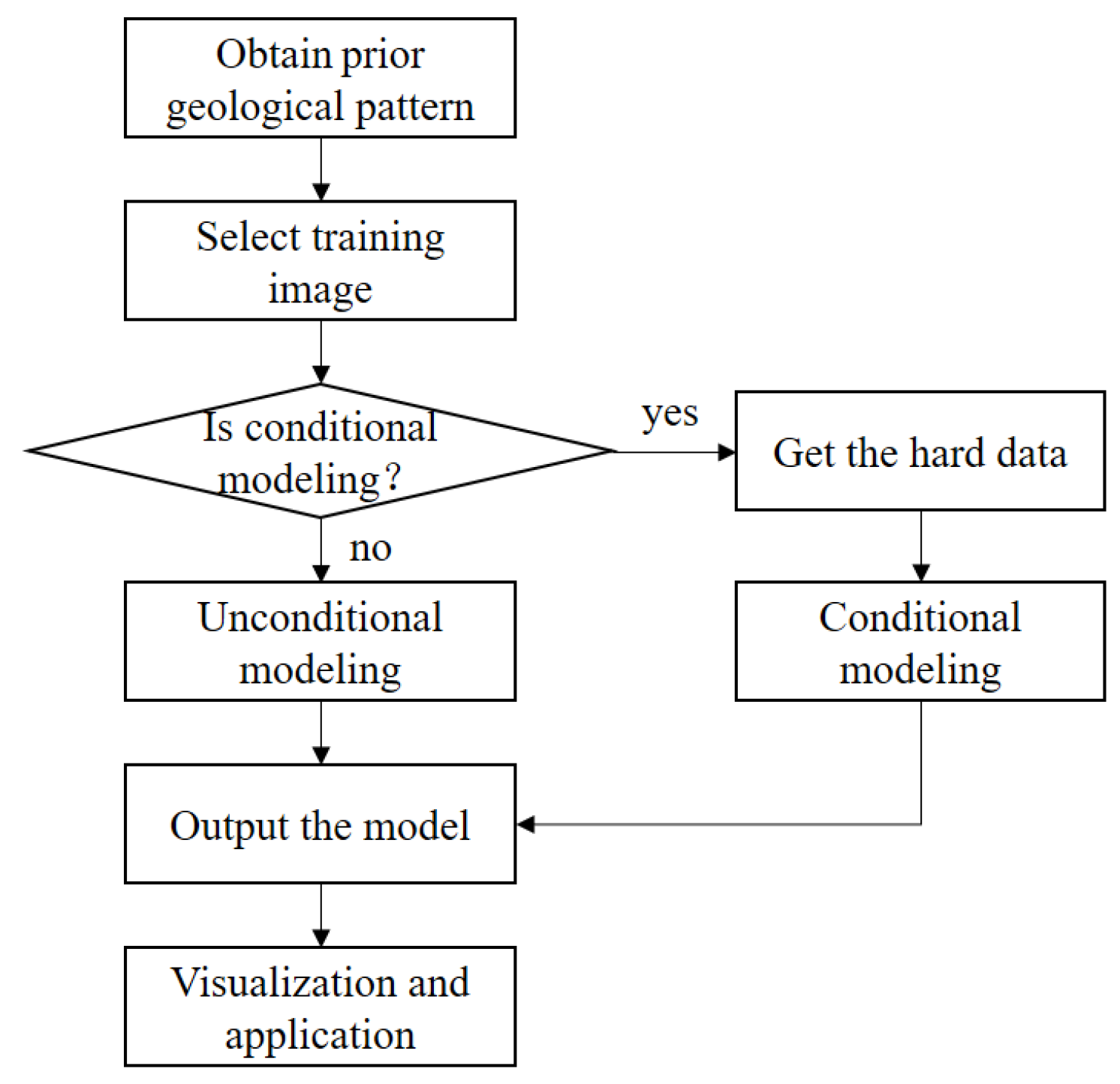
3.5. Modeling Workflow

Based on above research, a facies modeling workflow is proposed (shown in Figure 8). Firstly, according to the regional geological research, the prior geological pattern is obtained, and the TIs which can reflect the pattern are selected. Then, according to the application scenarios, the method of unconditional or conditional modeling is selected to establish the facies models. In this paper, an application program based on the Tensorflow framework is written to realize the modeling workflow: ① reading and preprocessing of TIs and hard data; ② core algorithm of improved method of reservoir facies modeling based on GANs; ③; output models in various formats, including image format (.jpg file) and petrel® model format (.grdecl file), etc.

4. Verification and Application

4.1. Verification

Taking the complex and common sand bodies of meandering river main channel and delta plain distributary channel as examples, the TIs for multi-point geostatistics are used as test data to verify the effectiveness of reservoir facies modeling method based on GANs to deal with stationary and non-stationary problems. Ten thousand TIs of sand bodies of meandering river main channel (Figure 9a) and delta plain distributary channel (Figure 9b) with grid size of 100 × 100 were selected to provide prior geological patterns for GANs. It is noted that the realizations are not relied on any specific TIs but generated according to the overall patterns, which means the generated realizations can be more than concrete TIs. Although the number of TIs is not strictly required, more TIs may help the diversity and facticity of realizations. Build a deep convolution generation adversarial network for reservoir facies modeling (Figure 5): ① the generator network has four deconvolution layers, including 512, 256, 128 and 64 deconvolution kernels, respectively, the input is a number of vectors of size 1 × 200, and the output is the same number of reservoir facies models with grid size of 100 × 100; ② the discriminator network has four convolution layers, including 64, 128, 256 and 512 convolution kernels, respectively, the input is the generated reservoir facies models with grid size of 100 × 100, the output is the results of discrimination whether these models are true or false; ③ the kernels size is 5 × 5, 7 × 7 or 9 × 9, and the convolution step size is set up to 2; ④ in conditional loss function, 2-norm is selected and the α is set up to 10 for conditional modeling.

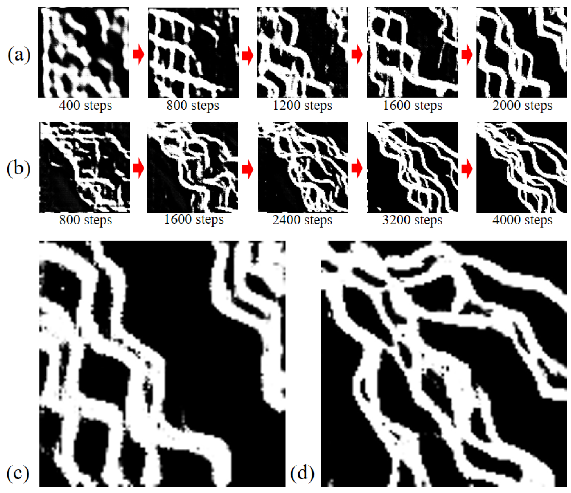
4.1.1. Unconditional Modeling

For the sand bodies of meandering river main channel and sand bodies of delta plain distributary channel, the intermediate results of training are shown in Figure 10a and Figure 10b, respectively, after 2000 and 4000 steps of training, the morphology of sand bodies is gradually formed. One of realizations of above two unconditional modeling are shown in Figure 10c,d. These results show that the method can effectively learn and reproduce the complex prior geological patterns, and has good modeling effect for both stationary and non-stationary problems.

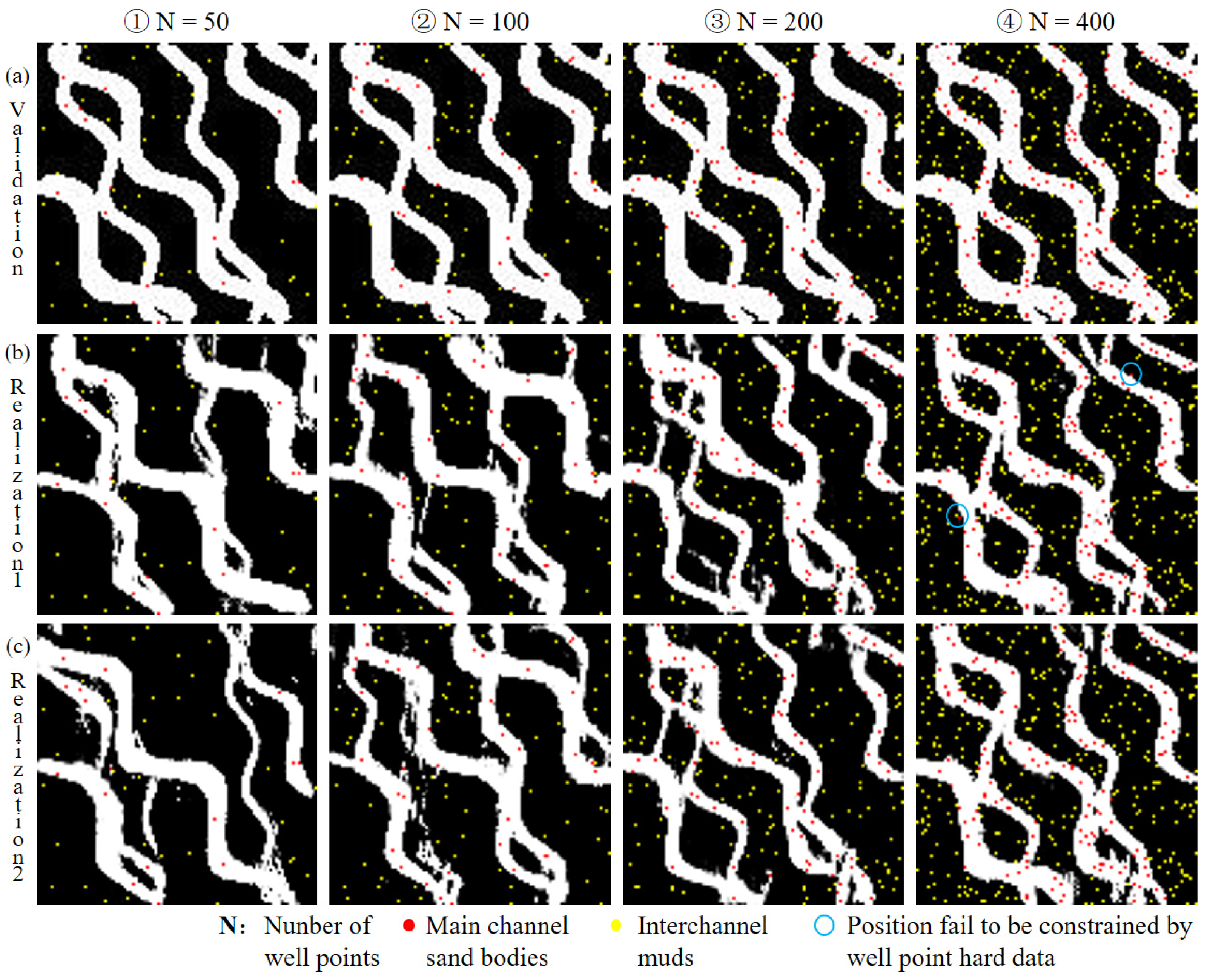
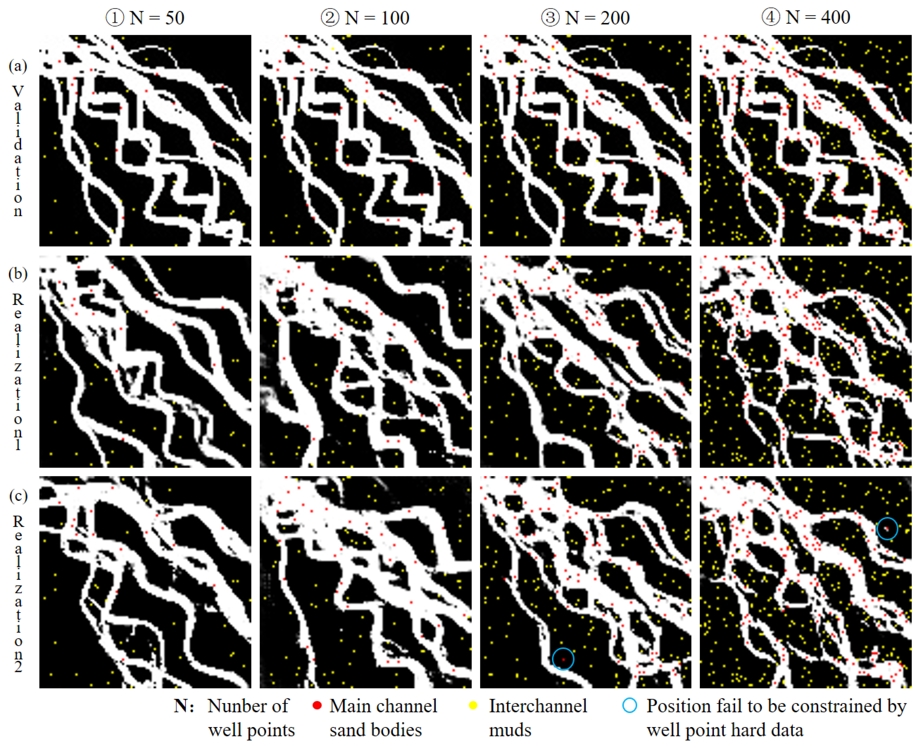
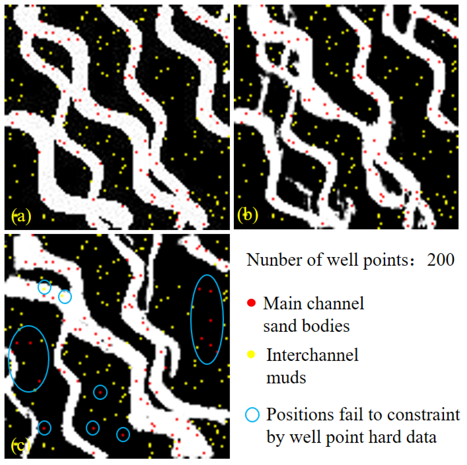
4.1.2. Conditional Modeling
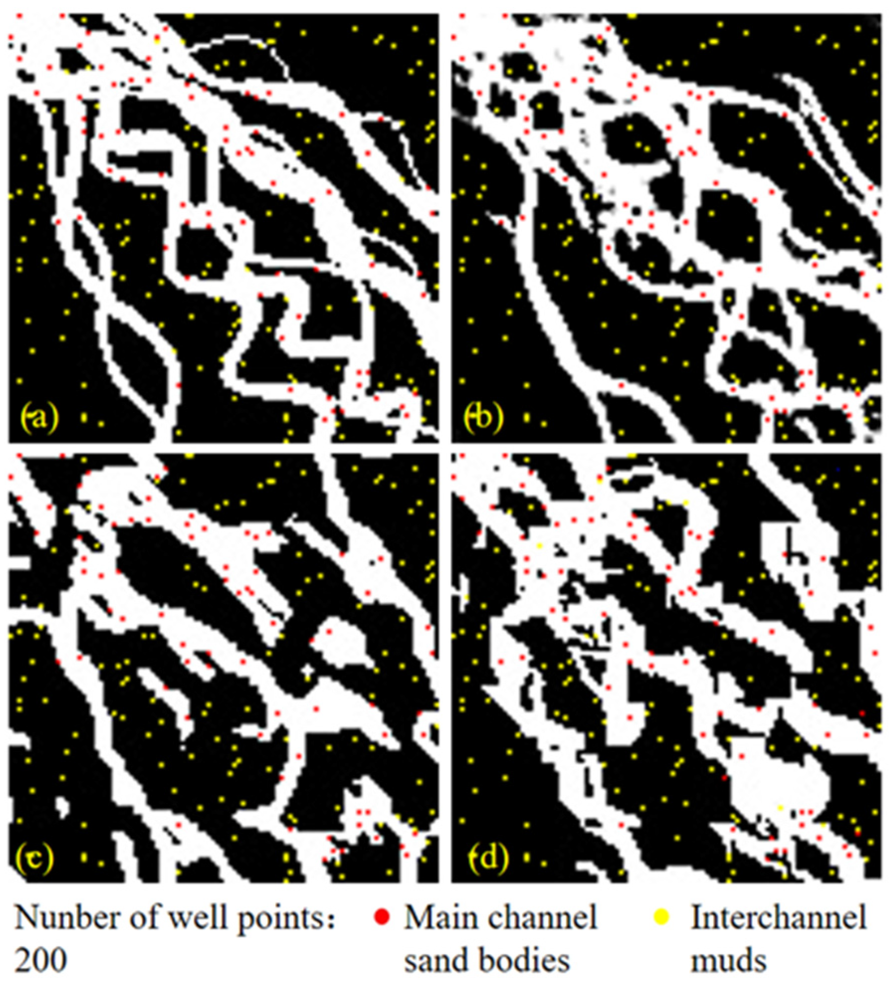
Another image is selected from the test dataset as validation data, and 50, 100, 200 and 400 points are randomly selected as well point to provide constraints information (Figure 11a and Figure 12a).
For the sand bodies of meandering river main channel, the modeling results are shown in Figure 11b. The models established under the constraints of different number (N) of well points reflect well the morphology of sand bodies, and basically honor the hard data at well points (Table 1). In addition, with the increase of the number of well points, the morphology of sand bodies in the realizations are more similar to that in the verification data, which indicates that the method can realize the effective constraints of hard data on facies modeling.
For the sand bodies of delta plain distributary channel, the modeling results are shown in Figure 12b. The models reflect the sand bodies morphology and realize the reproduction of the prior geological pattern. Meanwhile, the well point position matched the hard data (Table 1). Compared with the stationary meandering river main channel sand bodies, the non-stationary delta plain distributary channel sand bodies are more challenging to the method: when the hard data is less, some channel sand bodies are missing due to the lack of hard data constraints; when the hard data is increased, a small number of well points fail to match in order to meet the morphology of sand bodies. Although there are a few discontinuous channels in the modeling results, the overall effect is still good.
The above test results show that the method can not only realize the condition modeling of stationary problems, but also have a good modeling effect on complex non-stationary problems.

4.2. Comparison

Firstly, it is compared with multi-point geostatistics. As shown in Figure 13, the UCSC method (Figure 13b), the probability-based multi-point geostatistics method (Snesim) [7] (Figure 13c) and the pattern-based multi-point geostatistics method (Filtersim) [9] (Figure 13d) are used to facies modeling under the same hard data constraints. Snesim and Filtersim are the most commonly used multi-point geostatistics methods in facies modeling. The results show that all the three methods can be honor to well point constraints, but UCSC method can better reproduce the non-stationary prior geological pattern, and the resulting delta plain distributary channel sand bodies has stronger continuity and closer morphological characteristics to the verification model, which has obvious advantages.
Then, it is compared with D-Z method. As shown in Figure 14, the UCSC method (Figure 14b) and the D-Z method (Figure 14c) are used to facies modeling under the same hard data constraints. Modeling results of two methods both meet the prior geological pattern well, but the facies model established by D-Z method fails to honor the hard data at some well points, which indicates that the conditional constraint of D-Z method is insufficient, and makes it difficult to adequately adjust the distribution and morphology of sedimentary microfacies according to the hard data. UCSC method can better overcome this shortcoming.

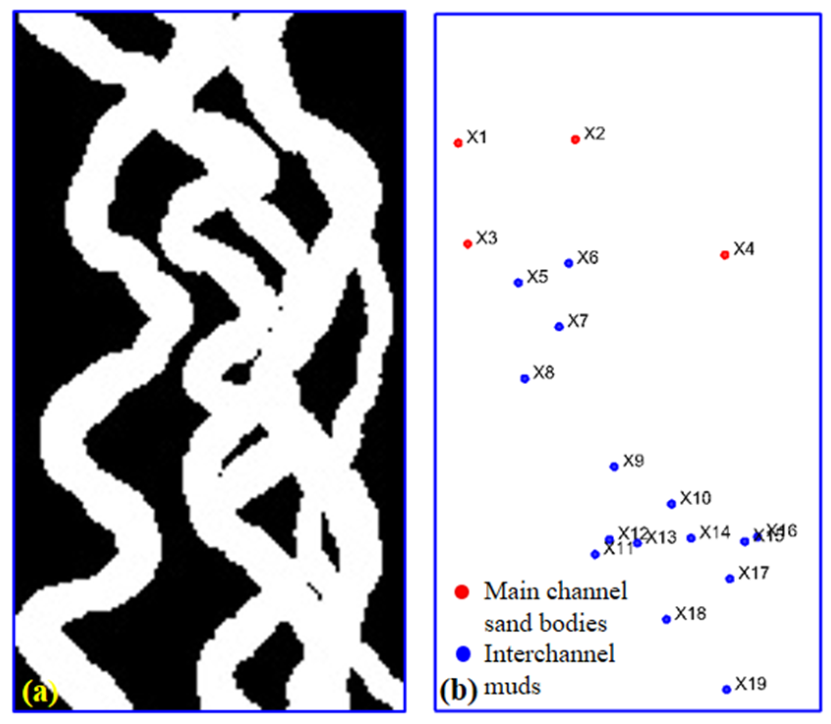
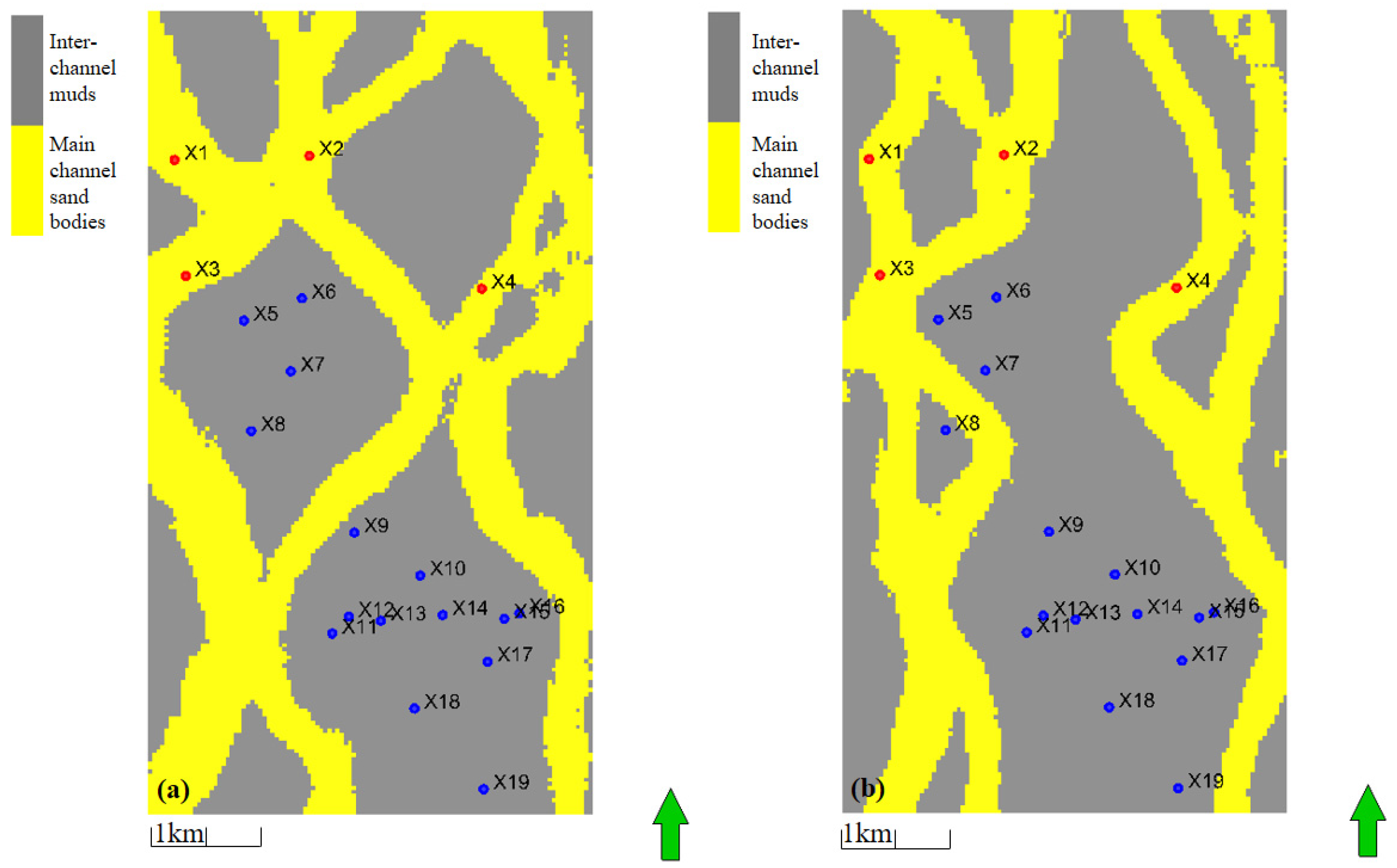
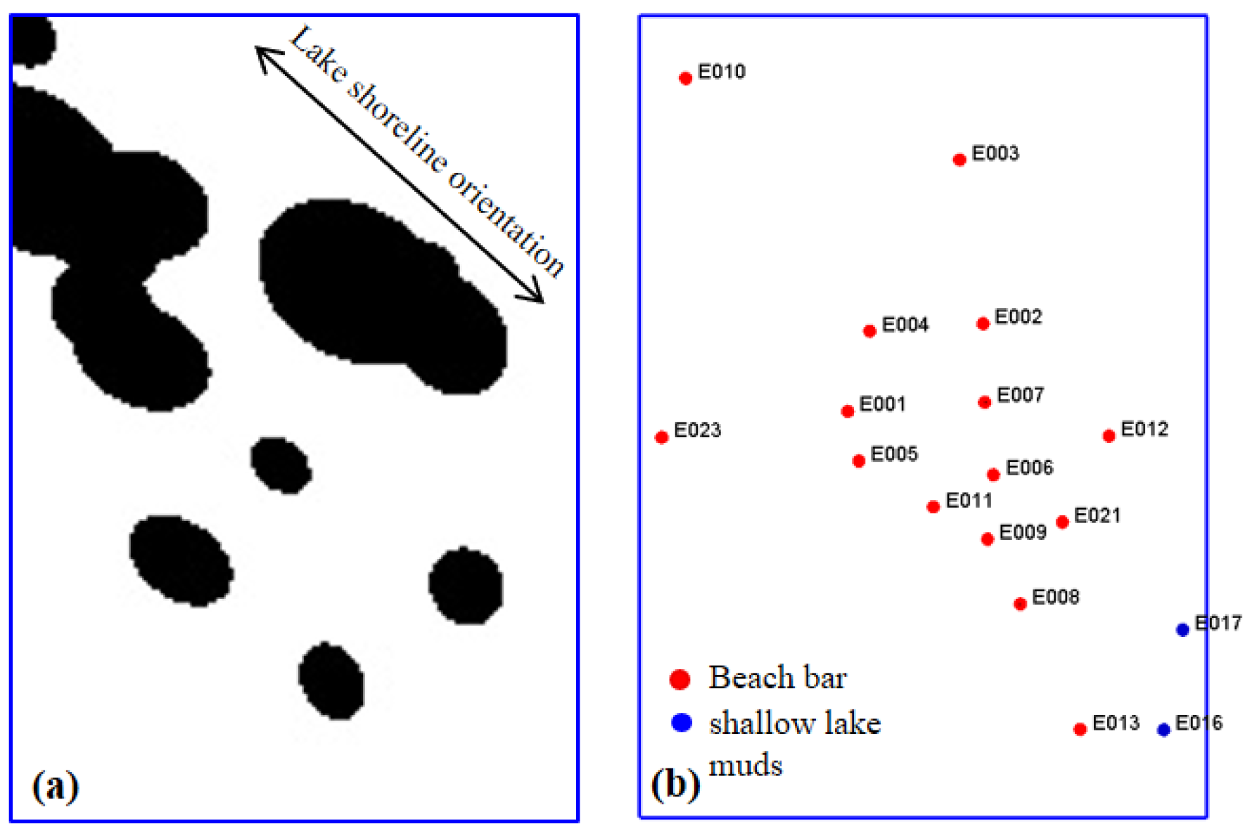
4.3. Application Examples

Taking the facies modeling of two typical continental reservoirs in China as examples, the suitability and practicability of the method is verified by using the actual oilfields data. Firstly, taking the NG1 layer of Neogene Guantao formation in X area of Shengli Oilfield as an example, the reservoir facies model is established. The NG1 layer in this area is dominated by fluvial facies, mainly developed meandering river deposits, the channels of meandering river are not fixed and often changed [23]. Based on the prior geological pattern, 5000 TIs (Figure 15a) are selected for training, and the sedimentary microfacies interpretation results of 19 wells are used as constraints (Figure 15b). Two realizations of modeling are shown in Figure 16, they honor the hard data at well points and meet the fluvial facies characteristics of the target layer perfectly [23,24].
Taking the E area in Xinjiang Oilfield as an example, the reservoir facies model is established with SC2 layer of Permian Lucaogou formation as the target layer. SC2 layer is mainly composed of beach bar deposits of shallow lake facies. The beach bars are often parallel or oblique to the lake shoreline, and distributed wide in sheet form [2]. Based on this prior geological pattern, 5000 TIs (Figure 17a) were selected for training, and the sedimentary microfacies interpretation results of 17 wells are used as constraints (Figure 17b). Two realizations of the modeling are shown in Figure 18, which honor the hard data at well points and meet the understanding of distribution of beach bar sand bodies and shallow lake muds [2]. Meanwhile, the beach bar microfacies distribution of established models have a certain indication significance for the sweet spot area of this layer, in which two horizontal wells, E002_H and E024_H, obtained high yield.
The above test results show that UCSC method has good practicability and application prospect: (1) it is not only suitable for specific square model (as shown in Section 4.1 with a grid size of 100 × 100), but also for grid size determined by actual data (such as X area and E area with grid size of 197 × 109 and 185 × 130); (2) it is capable of combining perfectly the continental sedimentary pattern of the actual areas with the wells data to describe different target layers; (3) in practice, while the pattern and hard data are given, it can provide a certain numbers of reasonable realizations conveniently to geologist for helping in efficiency increasing, assessment and decision making.

5. Conclusions and Discussion

In this paper, an improved method of reservoir facies modeling based on GANs is proposed, which realizes the unconditional and conditional modeling of stationary and non-stationary geological patterns, and provides a new idea and method for the modeling of continental sedimentary reservoir facies. Compared with the traditional geostatistics methods, this method significantly improves the capability of learning and reproducing the complex prior geological patterns, especially in modeling of non-stationary facies, such as sand bodies of delta plain distributary channel. Compared with the existing GANs based methods, this method has better conditional constraint effect that the results honor almost strictly the well point constraints meanwhile maintaining geological patterns. In practical applications, this method shows the good suitability and practicability prospect, it can establish reservoir facies models with different grid size according to actual oil field data and provide a certain number of reasonable realizations, which conveniently helps geologists to increase modeling efficiency and make decisions such as the realizations indicated the sweet spot in area E.
For application of the method and future research, such as the deep learning models that we used in verification obtain good performances, their hyperparameter settings can be a reference. However, for handling new cases, tuning modestly by trial and error method to find a more suitable hyperparameter settings is suggested, even if it is hard to exhaust all the settings and find the best.
GANs have the advantage of complex reservoir facies modeling because of its strong pattern generation capability, but the facies modeling method based on GANs still needs to be further improved. In method, it needs further research on the constraint by seismic data; in application, the unconditional modeling method based on GANs can also use remote sensing big data to realize extensive learning of modern sedimentary pattern, and provide more realistic TIs for various reservoir facies modeling methods.

Author Contributions

Conceptualization, Q.L. and M.P.; methodology, Q.L.; software, Q.L.; validation, Q.L. and J.Y.; formal analysis, Q.L. and J.Y.; investigation, Q.L., W.L. and J.Y.; resources, W.L.; data curation, Q.L., W.L. and Y.L.; writing—original draft preparation, Q.L.; writing—review and editing, M.P.; visualization, Q.L.; supervision, M.P. and W.L.; project administration, M.P.; funding acquisition, W.L. and Y.L. All authors have read and agreed to the published version of the manuscript.

Funding

This work was funded by Major National Science and Technology Projects of China (no. 2017ZX05013-002-002) and Major National Science and Technology Projects of China (no. 2016ZX0510-001).

Acknowledgments

The authors would like to thank the anonymous reviewers for the valuable comments.

Conflicts of Interest

The authors declare no conflict of interest.

References

  1. Wu, S.H.; Li, Y.P. Reservoir modeling: Current Situation and Development Prospect. Mar. Orig. Pet. Geol. 2007, 12, 53–60. [Google Scholar]
  2. Zhang, Y.Q.; Ma, S.Z.; Gao, Y.; Li, Y.Y.; Zhang, J.; Wang, L.; Sun, Y.; Xu, F.Z.; Li, H. Depositional Facies Analysis on Tight Reservoir of Lucaogou Formation in Jimsar Sag, Junggar Basin. Acta Sedimentol. Sin. 2017, 35, 358–370. [Google Scholar]
  3. Yang, S.C.; Zhao, X.D.; Zhang, X. Prediction of “sweet spots” of tight sandstone gas reservoirs in Jishen 1 area, Turpan-Hami Basin. J. Xi’an Shiyou Univ. Nat. Sci. Ed. 2014, 29, 1–8. [Google Scholar]
  4. Kovalevski, E.B. Geological Modeling Based on Geostatistics; Petroleum Industry Press: Beijing, China, 2014. [Google Scholar]
  5. Krige, D.G. A Statistical Approach to Some Basic Mine Valuation Problems on the Witwatersrand. J. Chem. Metall. Min. Soc. S. Afr. 1951, 94, 95–111. [Google Scholar]
  6. Matheron, G. Principles of geostatistics. Econ. Geol. 1963, 58, 1246–1266. [Google Scholar] [CrossRef]
  7. Strebelle, S. Sequential Simulation Drawing Structures from Training Images. Ph.D. Thesis, Stanford University, Stanford, CA, USA, 2000. [Google Scholar]
  8. Aprat, B.G.; Caers, J. A Multi-Scale, Pattern-Based Approch to Sequantial Simulation; Stanford Center for Reservoir Forecasting: Stanford, CA, USA, 2003. [Google Scholar]
  9. Zhang, T.F.; Switzer, P.; Journel, A. Filter-Based Classification of Training Image Patterns for Spatial Simulation. Math. Geol. 2006, 38, 63–80. [Google Scholar] [CrossRef]
  10. Caers, J.; Ma, X. Modeling Conditional Distributions of Facies from Seismic Using Neural Nets. Math. Geosci. 2002, 34, 143–167. [Google Scholar]
  11. Caers, J.; Zhang, T.F. Multiple-point Geostatistics: A Quantitative Vehicle for Integrating Geologic Analogs into Multiple Reservoir Models. AAPG Mem. 2004, 80, 383–394. [Google Scholar]
  12. Zou, C.N. Unconventional Petroleum Geology, 2nd ed.; Geological Publishing House: Beijing, China, 2013. [Google Scholar]
  13. Goodfellow, I.J.; Pouget-Abadie, J.; Mirza, M.; Xu, B.; Warde-Farley, D.; Ozair, S.; Courville, A.; Bengio, Y. Generative Adversarial Networks. Adv. Neural Inf. Process. Syst. 2014, 3, 2672–2680. [Google Scholar]
  14. Radford, A.; Metz, L.; Soumith, C. Unsupervised representation learning with deep convolutional generative adversarial networks. arXiv 2015, arXiv:1511.06434. [Google Scholar]
  15. Caers, J.; Journel, A.G. Stochastic Reservoir Simulation Using Neural Networks Trained on Outcrop Data; SPE Annual Technical Conference and Exhibition: New Orleans, LA, USA, 1998. [Google Scholar]
  16. Cao, K. Key Techniques of 3-D Property Modeling Based on Multiple-Point Simulation. Ph.D. Thesis, Peking University, Beijing, China, 2017. [Google Scholar]
  17. Chan, S.; Elsheikh, A.H. Parametrization and Generation of Geological Models with Generative Adversarial Networks. arXiv 2017, arXiv:1708.01810. [Google Scholar]
  18. Laloy, E.; Hérault, R.; Jacques, D. Training-image based geostatistical inversion using a spatial generative adversarial neural network. Water Resour. Res. 2018, 54, 381–406. [Google Scholar] [CrossRef] [Green Version]
  19. Dupont, E.; Zhang, T.F.; Tilke, P. Generating Realistic Geology Conditioned on Physical Measurements with Generative Adversarial Networks. arXiv 2018, arXiv:1802.03065. [Google Scholar]
  20. Zhang, T.F.; Tilke, P.; Dupont, E. Generating Geologically Realistic 3D Reservoir Facies Models Using Deep Learning of Sedimentary Architecture with Generative Adversarial Networks. In Proceedings of the International Petroleum Technology Conference, Beijing, China, 26–28 March 2019. [Google Scholar]
  21. Avalos, S.; Ortiz, J.M. Geological modeling using a recursive convolutional neural networks approach. arXiv 2019, arXiv:1904.12190. [Google Scholar]
  22. Kim, J.; Kim, S.; Park, C.; Lee, K. Construction of prior models for ES-MDA by a deep neural network with a stacked autoencoder for predicting reservoir production. J. Pet. Sci. Eng. 2020, 187, 106800. [Google Scholar] [CrossRef]
  23. Yang, P.J. Multiple-points geostatistics stochastic simulation based on patterns clustering and matching. Prog. Geophys. 2018, 33, 279–284. [Google Scholar]
  24. Zhang, Z.M. Development and tendency of techniques for fluvial reservoir description in Shengli shallow beach sea. Prog. Geophys. 2017, 32, 822–826. [Google Scholar]
Figure 1. Variogram of two-point geostatistics is hard to characterize sufficiently the geological heterogeneity (modify according to reference [11]). (ac) Three different geological heterogeneities; (d) Variograms in east–west; (e) Variograms in north–south.
Energies 14 03873 g001
Figure 2. Multi-point geostatistics is hard to reproduce the non-stationary geological patterns (modify according to reference [11]). (a) The training image with non-stationary geological patterns; (b) one realization produced by multi-point geostatistics.
Energies 14 03873 g002
Figure 3. GANs is successfully applied in image generation and there are similarities between facies models and specific images. (a) Image generated by GANs [14]; (b) Remote sensing image of modern river channel; (c) Model of anastomosing river channel.
Energies 14 03873 g003
Figure 4. Schematic diagram of implementation of generative adversarial networks.
Energies 14 03873 g004
Figure 5. Schematic diagram of architecture of deep convolutional generative adversarial networks.
Energies 14 03873 g005
Figure 6. Schematic diagram of the improved method of unconditional simulation modeling and conditional simulation modeling based on GANs.
Energies 14 03873 g006
Figure 7. Schematic diagram of implementation of conditional loss function.
Energies 14 03873 g007
Figure 8. Workflow of facies modeling using improved GANs method.
Energies 14 03873 g008
Figure 9. Examples of training images. (a) Training images for sand bodies of meandering river main channel; (b) training images for delta plain distributary channel.
Energies 14 03873 g009
Figure 10. The results of unconditional modeling. (a) Unconditional modeling intermediate results of stationary problem; (b) unconditional modeling intermediate results of non-stationary problem; (c) unconditional modeling result of stationary problem; (d) unconditional modeling result of non-stationary problem.
Energies 14 03873 g010
Figure 11. Results of conditional modeling of stationary problem (meandering river main channel sand bodies). (a) The validation model; (b) a group of realizations constrained by different number of well points; (c) another group of realizations constrained by different number of well points.
Energies 14 03873 g011
Figure 12. Results of conditional modeling of non-stationary problem (delta plain distributary channel sand bodies). (a) The validation model; (b) a group of realizations constrained by different number of well points; (c) another group of realizations constrained by different number of well points.
Energies 14 03873 g012
Figure 13. The comparison of the conditional modeling results between UCSC method and the traditional method. (a) Validation model; (b) model established by UCSC method; (c) model established by Snesim; (d) model established by Filtersim.
Energies 14 03873 g013
Figure 14. The comparison of the conditional simulation modeling results between UCSC method and the D-Z method. (a) Validation model; (b) model established by UCSC method; (c) model established by D-Z method.
Energies 14 03873 g014
Figure 15. Training images and well point hard data of facies modeling of NG1 layer in X area of Shengli Oilfield. (a) Training images (b) well point hard data.
Energies 14 03873 g015
Figure 16. The facies model of NG1 layer in X area of Shengli Oilfield established by the UCSC method. (a) Realization1; (b) Realization2.
Energies 14 03873 g016
Figure 17. Training images and well point hard data of facies modeling of SC2 layer in E area of Xinjiang Oilfield. (a) Training images; (b) well point hard data.
Energies 14 03873 g017
Figure 18. The facies model of SC2 layer in E area of Xinjiang Oilfield established by the UCSC method. (a) Realization1; (b) Realization2.
Energies 14 03873 g018
Table 1. Well point coincidence rate of conditional modeling with different number of well point hard data constraints.
Number of Well PointsSand Bodies of Meandering River Main Channel (Stationary Problems, Figure 11)Sand Bodies of Delta Plain Distributary Channel (Non-Stationary Problems, Figure 12)
Realization1Realization2Realization1Realization2
50100%100%100%100%
100100%100%100%100%
200100%100%100%99.75%
40099.5%100%100%99.75%
Publisher’s Note: MDPI stays neutral with regard to jurisdictional claims in published maps and institutional affiliations.

