An RTDS-Based Testbed for Investigating the Impacts of Transmission-Level Disturbances on Solar PV Operation

Abstract

The increasing penetration of renewable energy resources such as solar and wind via power electronic inverters is challenging grid dynamics, as well as grid planning, operation, and protection. Recently, the North American Electric Reliability Corporation (NERC) has reported a series of similar events of the unintended loss of solar generation in Southern California over a large geographic area following the transmission-level disturbances. These events highlight the importance of understanding the characteristics of the transmission-side disturbances propagating into the distribution systems and their impacts on the operation of inverter-based resources. In this paper, a real-time electromagnetic simulation testbed is constructed for real-time electromagnetic simulations to generate realistic transmission-level disturbances and investigate their impacts on the solar PV operation under different fault types and locations, solar penetration levels, and loading levels. Through the simulation analysis and grid strength assessment, it is found that the grid strength at points of integration (POIs) of solar PVs significantly affects the transient stability of solar generators. Particularly, undesirable transient stability events are more likely to occur at the weak POIs following the transmission-level disturbances. Moreover, undesirable transient stability events become severer when the transmission-level disturbance is closer to the weak POIs or the disturbances become more serious. Additionally, the impact of the transmission-level disturbances on the solar PVs at the weak POIs exacerbate with the increasing solar penetration levels and loading levels. Thus, it is important to study and develop new technologies for grid planning, operation, and protection in weak grid conditions to address the emerging issues of integrating the high penetration of solar PVs and other IBRs.

1. Introduction

The electric power grid is undergoing a rapid change driven by the high penetration of renewable energy resources such as solar and wind via power electronic inverters. While these inverter-based resources (IBRs) can use power electronic controls to respond to grid disturbances nearly instantaneously and thus support grid reliability, they are challenging grid planning, operation, and protection [1]. The North American Electric Reliability Corporation (NERC) recently reported a series of similar events of the unintended loss of solar generation following the transmission-level disturbances that occurred from 2016 to 2020 in the Southern California region of the Western Electricity Coordinating Council’s footprint [1,2,3,4].

• On 16 August 2016, the transmission system owned by Southern California Edison experienced thirteen 500 kV line faults, and the system owned by the Los Angeles Department of Water and Power experienced two 287 kV faults as a result of the fire. The most significant event resulted in the loss of nearly 1200 MW. There were no solar PV facilities de-energized as a direct consequence of the fault event; rather, the facilities ceased output as a response to the fault on the system [1].
• On 9 October 2017, the fire caused two transmission system faults near the Serrano substation, east of Los Angeles. The first fault was a normally cleared phase-to-phase fault on a 220 kV transmission line, and the second fault was a normally cleared phase-to-phase fault on a 500 kV transmission line. Both faults resulted in approximately 900 MW of solar PV generation loss [2].
• On 20 April 2018 and 11 May 2018, two similar events caused a loss of solar photovoltaic (PV) facilities in response to transmission line faults, though no generating resources were tripped as a consequence of either of the line outages [3].
• On 7 July 2020, the static wire on a 230 kV double circuit tower failed, causing a single-line-to-ground fault on both the #1 and #2 parallel circuits on the tower. The fault was cleared normally in about three cycles. In addition, a nearby 230 kV line relay incorrectly operated for an external fault. For this first fault event, approximately 205 MW of power reduction was observed at solar PV facilities in the Southern California region. After the #1 circuit was re-energized and held, the #2 line was re-energized and relayed back out due to a low-impedance three-phase fault that was cleared normally in 2.3 cycles. This second fault event experienced a larger 1000 MW reduction in solar PV output primarily due to the fact that it was a three-phase fault [4].

These similar events highlight the potential reliability impacts of IBRs including solar PV systems at both the distribution and transmission levels. Recently, these events have been investigated in [5,6,7,8,9,10,11,12,13,14,15]. To study the impact of IBRs on the bulk power systems, generic positive sequence dynamic stability simulations such as PSS/E are used with a simpler representation of IBRs and inverters in [5,6,7]. To more accurately capture the dynamics of the inverters’ response to actual grid events using generic positive sequence stability models, reference [8] identifies the modeling deficiencies in generic inverter models. In [9,10,11], aggregated models of IBRs are used instead of individually detailed models of IBRs. Reference [12] presents a coupled simulation method, in which the transmission network is first initialized in a dynamic simulation platform and then the recorded response is passed to the distribution network, which is simulated in quasi-static time-series simulations. In [13,14,15], the impacts of inverter operating modes and inverter parameters on the transient stability of the bulk transmission system are studied. However, the existing works do not investigate the impact of the transmission-level disturbances on IBR operation, which is important for the operation of inverter-based resources. Additionally, these existing works usually use positive sequence stability models and simple inverter modeling for simulation analysis. Such models may not be used in electromagnetic transient simulations for modeling intricate details with different inverter controls and accurately evaluating the IBRs’ response during abnormal events. In addition, the complete network topology of the transmissions system and the distribution system is ignored, which cannot be used for understanding the characteristics of the transmission-level disturbances propagating into the distribution systems.

To address these issues, a real-time electromagnetic simulation testbed is constructed based on a Real-Time Digital Simulator (RTDS) by integrating an IEEE standard transmission network into an IEEE distribution test feeder interfaced with solar PVs in multiple locations in this paper. With the testbed and grid strength assessment, the impact of the transmission-level disturbances on solar PV operation is investigated under different fault types and locations, solar penetration levels, and loading levels. The main contributions of the paper can be summarized as follows:

(1)

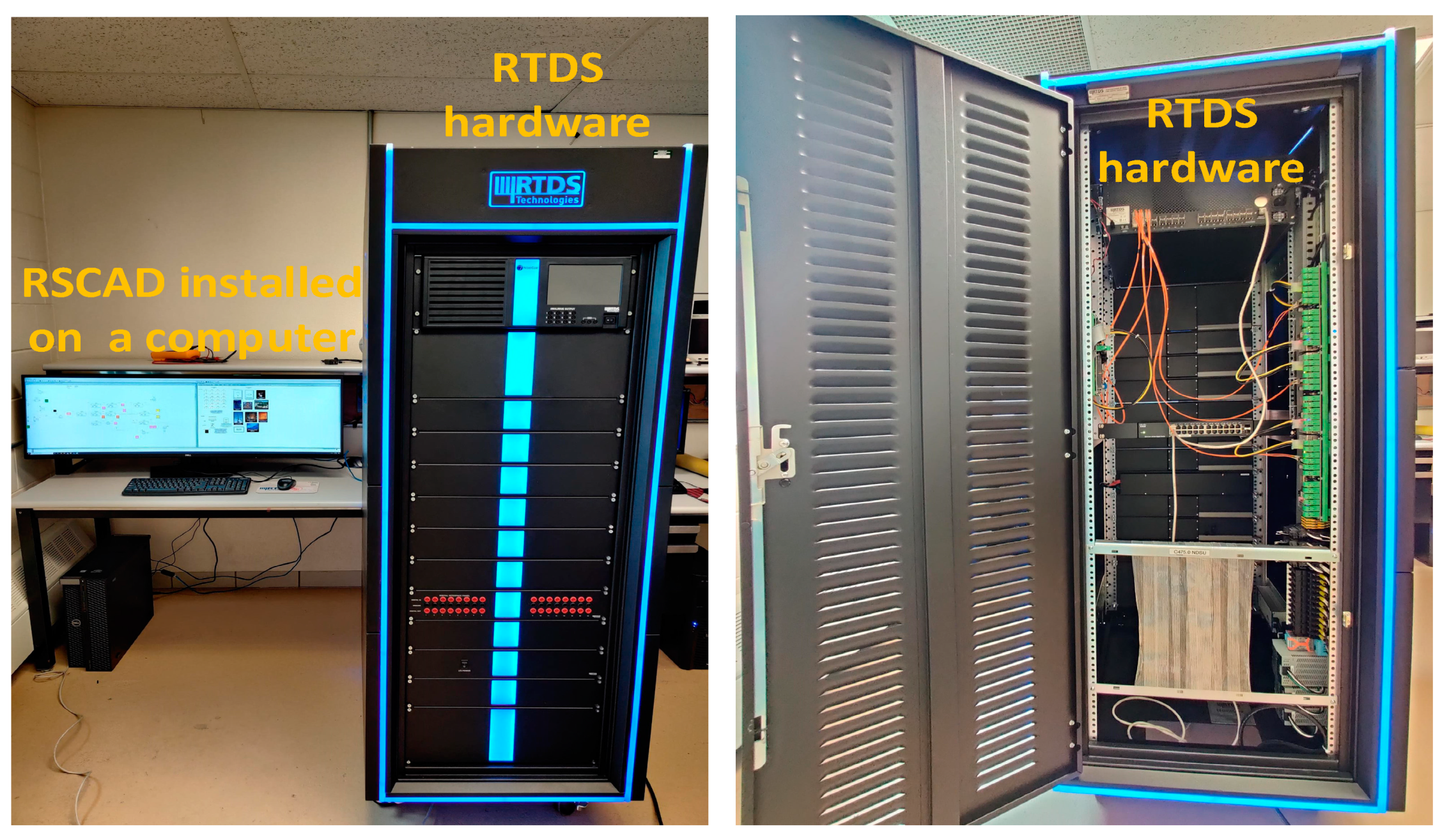
To generate realistic transmission-level disturbances and investigate their impacts on solar PVs in distribution systems, a real-time electromagnetic simulation testbed is constructed based on RTDS, which is developed by RTDS Technologies Inc. to solve the power system equations fast enough to realistically represent conditions in actual power grids [16].

(2)

The testbed has a full model of a transmission system, distribution system, and solar PVs. In the modeling of solar PVs, the detailed PV inverter controls are considered in the distribution system with the comprehensive models of synchronous machines and excitation in the transmission system.

(3)

By using this testbed to investigate the impact of the transmission-level disturbances on solar PV operation under different fault types and locations, solar penetration levels, and loading levels, it is found that the grid strength at different POIs significantly affects the transient stability of solar PV operation. Particularly, at the weak POIs, undesirable transient stability events are more likely to occur under increasing solar penetration levels or decreasing loading levels following severe transmission-level disturbances.

The rest of this paper is organized as follows: Section 2 presents the detailed modeling of the testbed created using RTDS, including the transmission system, distribution system, and the PV systems and their inverter controls; in Section 3, the impact of transmission-level disturbances on solar PV operation in the distribution system is investigated by using the real-time testbed under different fault conditions, solar penetration, and loading levels, and Section 4 provides additional discussion on the impact of grid strength on solar PV responses under different scenarios; finally, Section 5 concludes the paper.

2. RTDS-Based Testbed

2.1. RTDS

To generate realistic transmission-level disturbances and investigate their impacts on solar PVs in distribution systems, a real-time electromagnetic simulation testbed is constructed based on RTDS, which is a commercially available digital real-time power system simulator. RTDS is developed by RTDS Technologies Inc. in Winnipeg, Canada, for the simulation and analysis of electromagnetic transients in electric power systems. RTDS can solve the power system equation fast enough to continuously produce output conditions that realistically represent conditions in actual power grids.

RTDS is generally composed of hardware and software, which is shown in Figure 1. The RTDS hardware includes processing and communicating cards, which are inserted in the unit and connected to a common plate located in the back of the RTDS. The processing cards have a parallel processing architecture customized to simulate with one or multiple processors for the equation solution for the power system and its components. The communicating cards are used to handle the communication between RTDS and its software installed on the guest computer. RTDS has additional dedicated interface cards that allow the physical and logical connection between the simulated power systems and actual devices. The RTDS software is a graphic interface software, RSCAD, which allows users to build, compile, execute, and analyze simulation cases. This software has a wide library of power system components, control, and automated protection systems, as well as a friendly user interface, which can make the assembly and analysis of a wide variety of electric AC and DC systems easier and integrated. As shown in Figure 1, users can use RSCAD software to build a model representing the power system and load this model to the RTDS for the electromagnetic transient simulation while obtaining the updated states of the simulated power system model for analysis.

2.2. RTDS-Based Representative Power System Model

With RTDS, a representative power system model is constructed for real-time electromagnetic simulations to investigate the impact of transmission-level disturbances on the IBR operation in distribution systems. This model includes complete transmission and distribution systems with solar PVs. Figure 2 shows the single-line diagram of the constructed power system model. The component details in the model are described below.

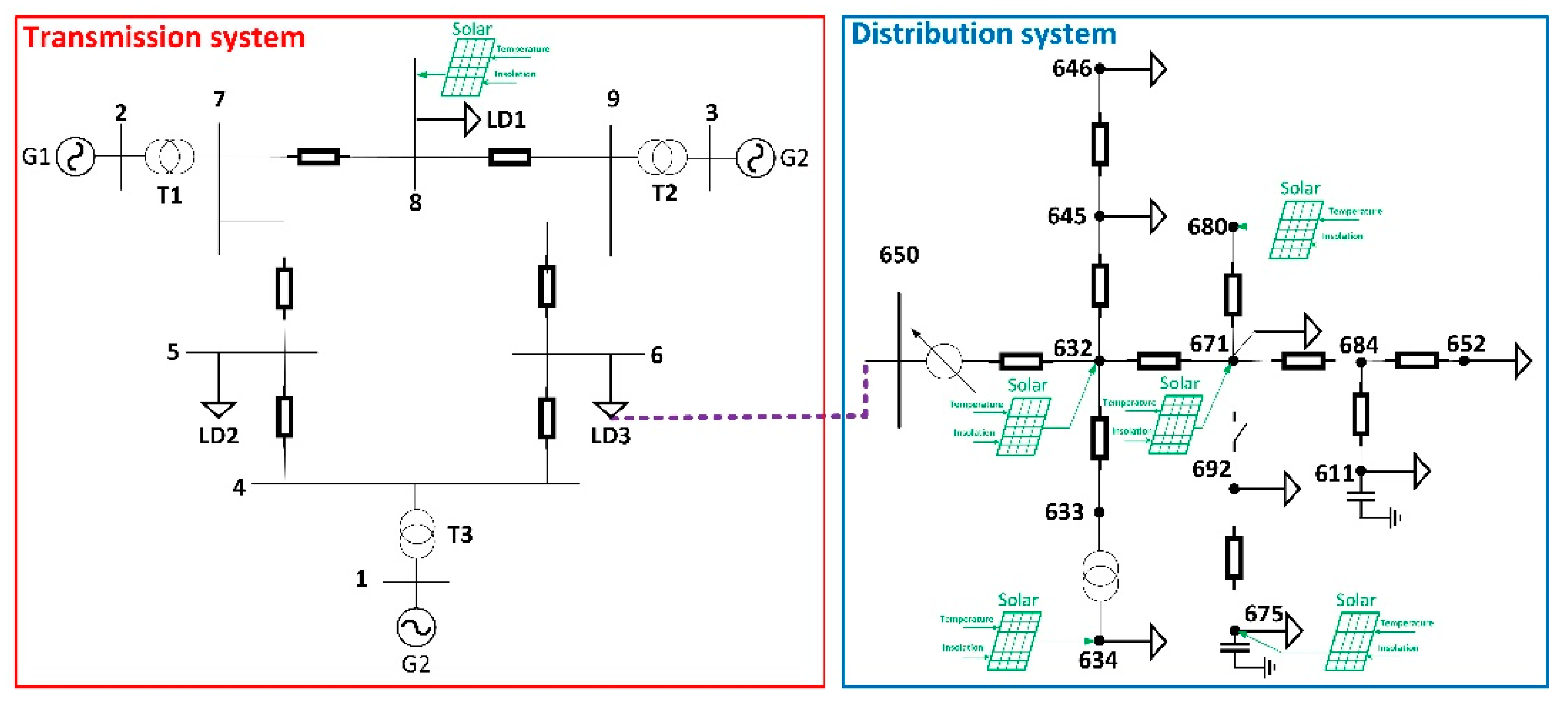
2.2.1. Transmission System

In the RTDS-based representative power system model, the transmission system is demonstrated by the IEEE 9 bus test system. In the system, its voltages include 230 kV at the transmission level and generator bus voltages of 16.5 kV, 18 kV, and 13.8 kV at buses 1, 2, and 3. The system is composed of three loads, three transformers, six transmission lines, and three synchronous generators with exciter and governor control systems. The system data can be found in [17]. The major electrical components used in the system include a hierarchy component box for the synchronous generator, the unified T-line model for the transmission line, and the dynamic load model.

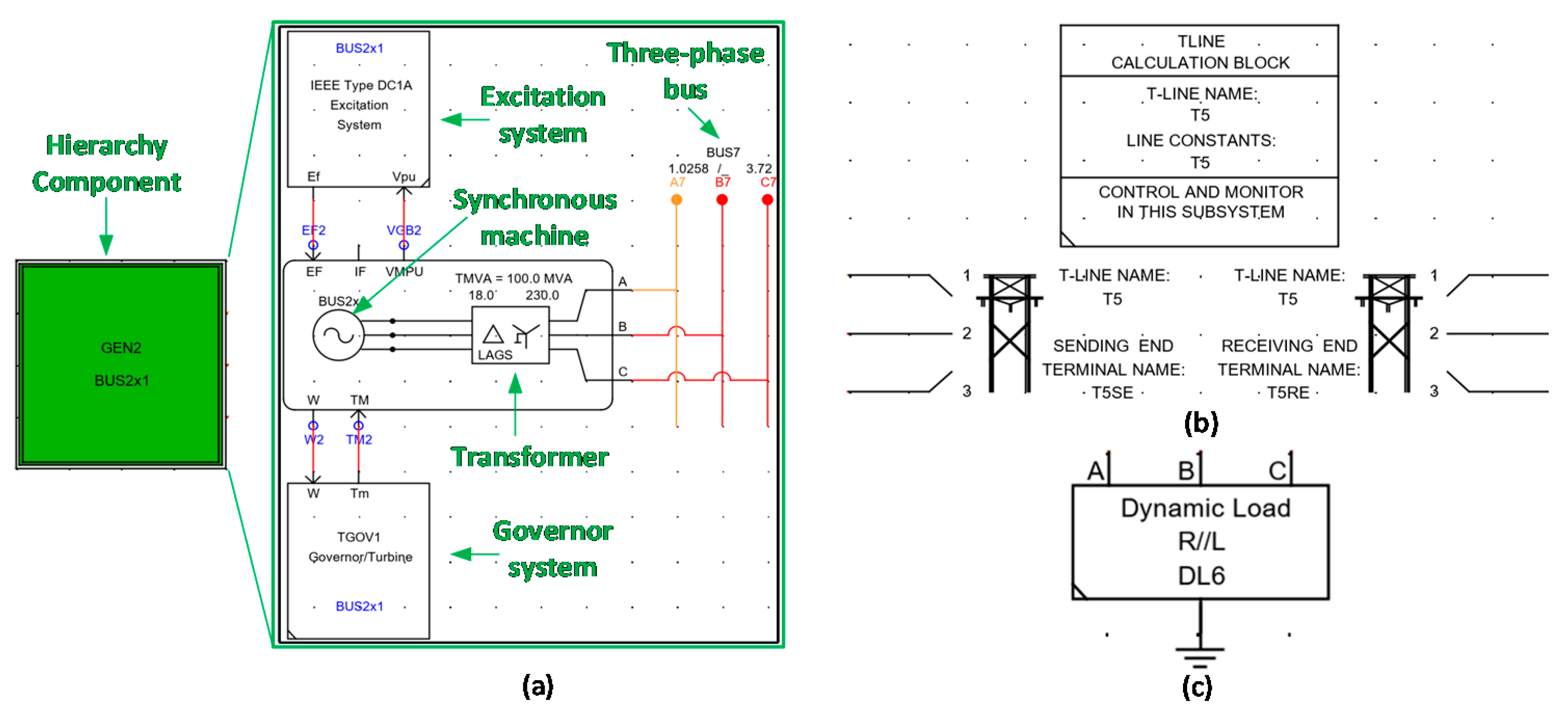
• The synchronous generator and its excitation and governor systems are represented by a hierarchy component box. As shown in Figure 3a, this hierarchy component box includes the models of a synchronous machine and its excitation and governor systems. All the synchronous machine systems are modeled with a steam turbine, a governor system and an excitation system. The excitation system is modeled with an AC excitation type (EXAC1A) model. The time constants, regulators, and feedback gains are the input parameters for the excitation system. The machine is connected to the transmission system via a transformer.
• The transmission lines in the system are represented by the unified T-line model. As shown in Figure 3b, the unified T-line model is composed of three electrical components: sending end, terminal end, and calculation box. The unified T-line model can be used for a Bergeron or a frequency-dependent phase model, but when required, either of these models can be collapsed into a simpler PI representation of a line. It is noted that in [9], the data are compensated for long line effects. The transmission lines in the RTDS simulation case are modeled using the Bergeron line model, which is simulated using distributed line parameters. Thus, the long line compensation was removed [15] to obtain the uncompensated data for the developed model.
• The load is represented by a dynamic load component in the transmission side of the network, which is shown in Figure 3c. The load model can be used to dynamically adjust the load to maintain real power and reactive power set points using variable conductance. Additionally, this model allows setting up the initial values and limits of real and reactive power absorbed by a load.

2.2.2. Distribution System

In the RTDS-based representative power system model, the distribution system is modeled by the IEEE 13 bus test feeder, which includes a two-winding transformer model, the PI section line model, dynamic load model, and a hierarchy component box for the voltage regulator [18].

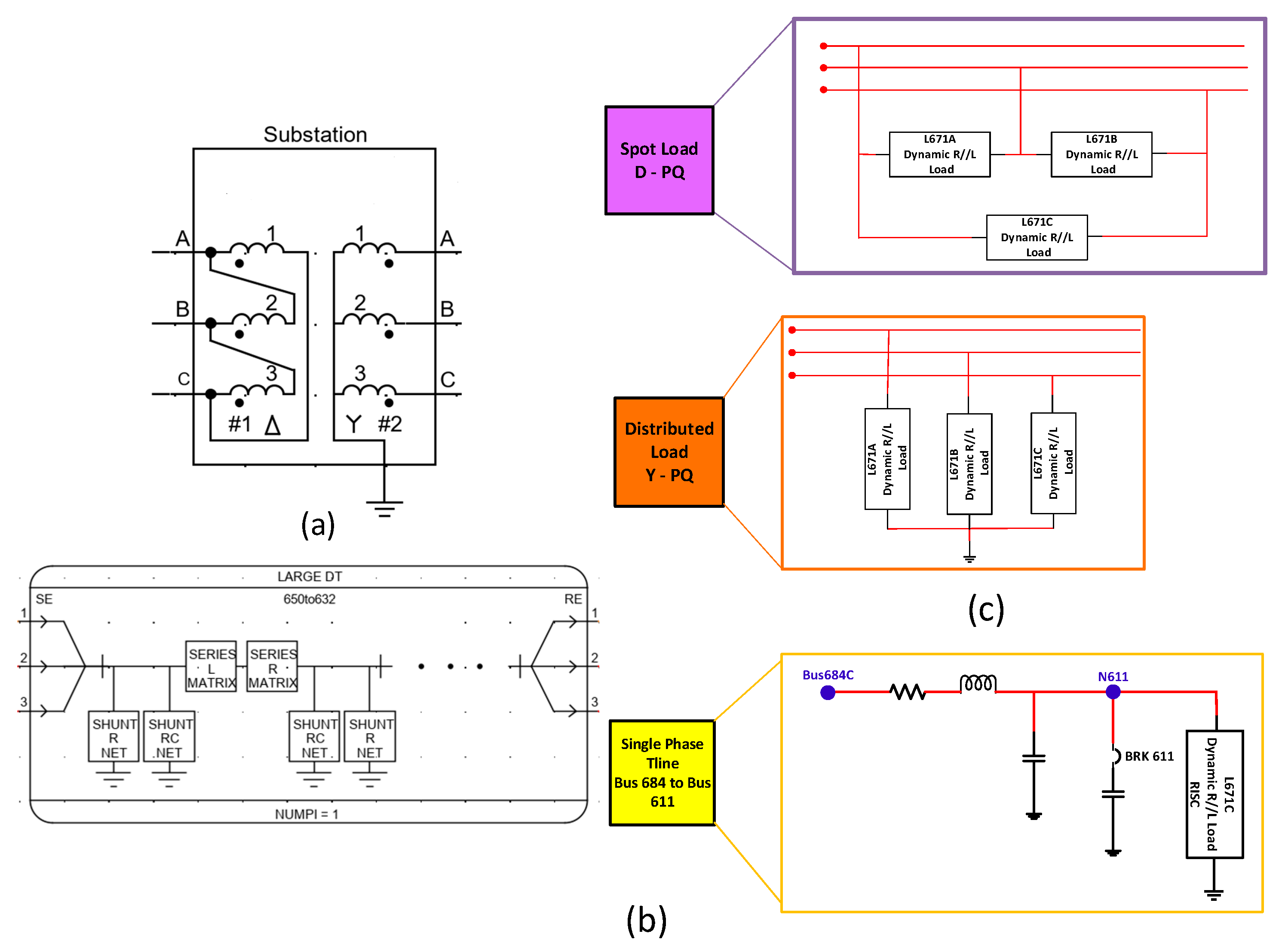
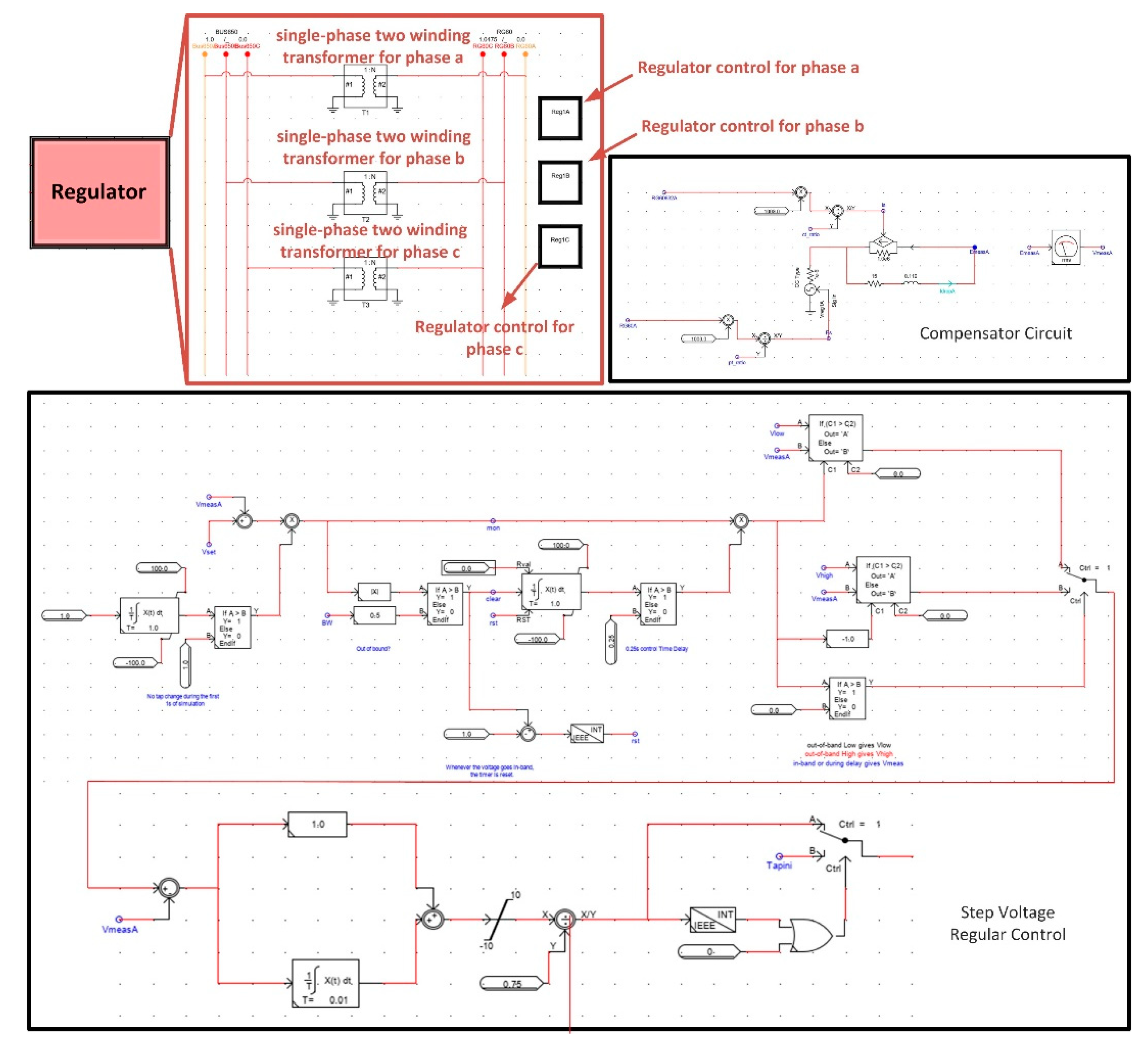
• In this system, a delta-wye transformer is connected to the transmission system, and it is represented by a two-winding, three-phase transformer model, which is shown in Figure 4a.
• The distribution line is represented by the PI section model in which a set of PI sections are connected in series, as shown in Figure 4b. It is noted that the PI section model requests the capacitance from the wire to the ground. The data given in [19] are the shunt capacitance matrix. Thus, the capacitance from the wire to the ground needs to be calculated from this matrix.
• The load in the system is represented by hierarchy component boxes. As shown in Figure 4c, different colored hierarchy component boxes include different connections of loads, which are modeled by the dynamic load component.

The voltage regulator has been adopted from the typical parameters used for the IEEE 13 bus test feeder. The voltage regulator is represented by a hierarchy component box. As shown in Figure 5, this hierarchy component box includes three single-phase two-winding transformers and the controls for the voltage regulator. For each phase, the regulator controls are represented by an individual hierarchy component box, in which there are the compensator circuit and the step voltage regulator control. This regulator is constructed based on reference [20].

2.2.3. Solar PV System

Solar PVs are integrated into the constructed transmission–distribution model. Each solar PV is modeled by the PV array component to supply the DC voltage for the converter. The converter is modeled using an average value model (AVM), and the AC side of the converter is connected to the feeder. Figure 6 shows the solar PV modeling components.

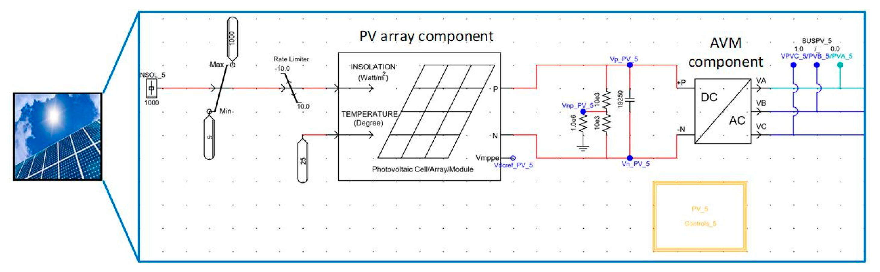
• A PV array model is used to represent the combination of individual solar cells into PV arrays to produce voltages and currents at the terminals of a PV array. The PV array generates power as a function of irradiation and temperature. The parameters of the PV array model can be modified to obtain a certain output power for the given irradiation and temperature. Each PV array has a temperature set to 25 °C and insolation to 1000 W/m² as input. This model can specify the parameters about how the cells are connected to form arrays. Additionally, this model can select different methods for estimating the maximum power point for a given insolation and temperature. The detailed parameters of the PV array are presented in

  Table 1. Parameters for solar PV system.

  Components	Parameters	Values
  PV	Number of series cells	36
  	Number of parallel strings	1
  	Open-circuit voltage (Voc)	21.7 V
  	Short-circuit current (Isc)	3.35 A
  	Number of modules in series	115
  	Number of modules in parallel	285
  	Voltage at Pmax	17.4 V
  	Current at Pmax	3.05 A
  DC link capacitor	Capacitance (Cdc)	5 mF
  Inverter	Filter resistance	1.0 mΩ
  	Filter inductance	100 μH
  High-pass filter	RH	0.039 Ω
  	LH	7.874 μH
  	CH	2500 μF
  Current control loop	kpi	0.2
  	kii	0.30675
  PLL	kpPLL	5
  	kiPLL	0.01

  .
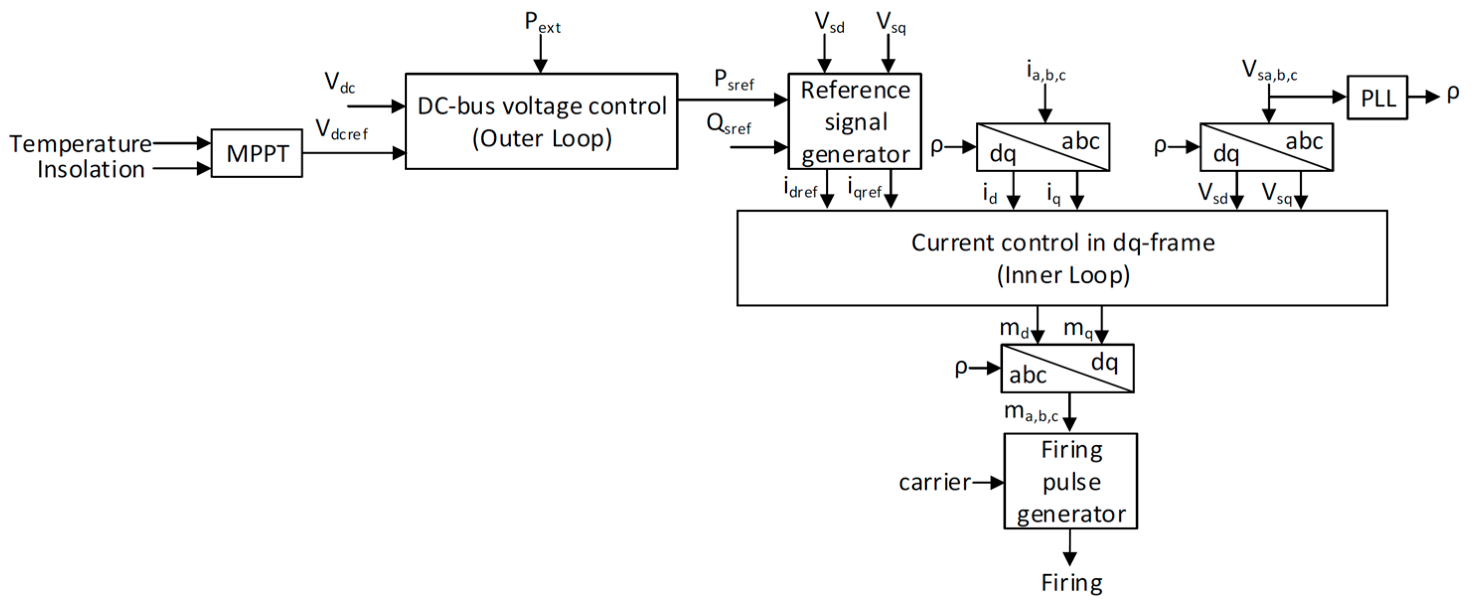
• The AVM component models the averaged converter control dynamics developed by equivalent voltage and current sources. As shown in Figure 7, solar PV controls use the maximum power point tracking (MPPT) algorithm, which computes the DC voltage set point required for maximum power transfer based on the temperature and insolation levels of the PV array. This DC voltage set point then feeds into the outer loop DC-bus voltage control, which computes a corresponding real power set point. The real and reactive power is then fed into the inner current control loop operating in the dq reference frame and a set of three-phase modulation waveforms is synthesized. These modulation waveforms are then used in a carrier-based, sinusoidal pulse width modulation (SPWM) strategy to generate a corresponding set of firing pulses.

3. Impact Analysis of Transmission-Level Disturbances on Distributed Solar PV Operation

With the transmission–distribution model constructed in Section 3, the impact of transmission-level disturbances on the operation of distributed solar PVs is investigated using the real-time electromagnetic transient simulation testbed based on RTDS. The performance of the transmission-distribution model is tested by comparing RTDS simulation results with those from PSCAD/EMTDC in terms of steady-state simulation testing and dynamic simulation testing. The steady-state simulation testing is focused on power flow solutions while the transient simulation testing was centered on the dynamics of voltage and current in the model under different faulted scenarios. The consistent results between RTDS simulation and PSCAD/EMTDC confirm the correct function of the constructed model. Due to the page limitation, the comparison results are not shown here. In the following transient simulation analysis, the simulation is performed based on the Dommel algorithm. The simulation time step is 100 µs, and the simulation time is 0.2 s. The transmission–distribution model has 114 nodes. In the model, five cases below are considered.

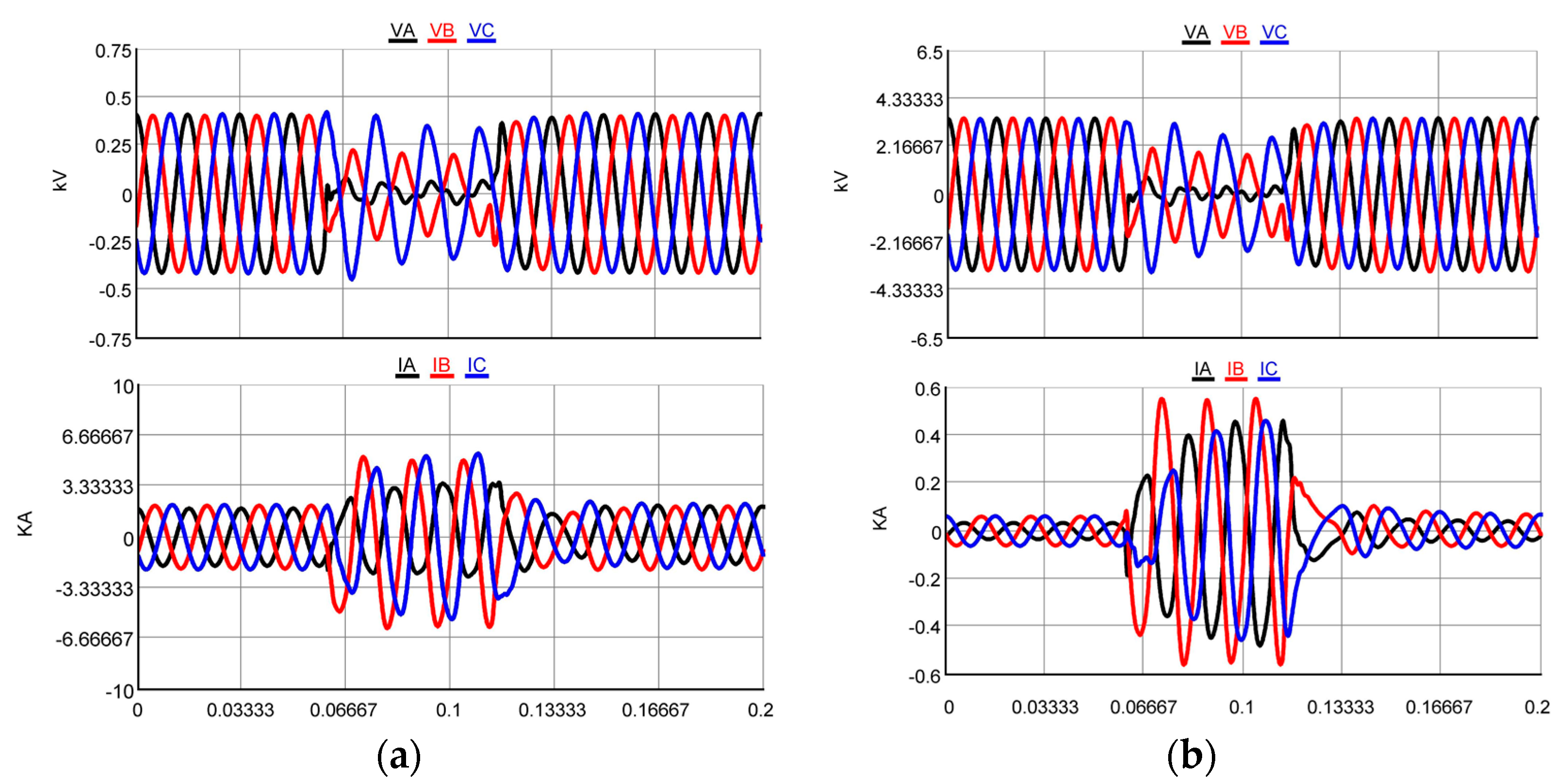
3.1. Impact of Fault Types in Transmission System on Solar PV Operation

In this case, different fault types in the transmission system are generated to investigate their impacts on the operation of solar PVs in the distribution system. The fault is applied at bus 6 in the transmission system. Four types of faults are considered, including a three-phase fault, a single line-to-ground fault, a line-to-line fault, and a double line-to-ground fault. Each type of fault has the same occurring and clearing times when it is applied at bus 6. Following different types of faults, the voltage and current of each solar PV bus in the distribution system are observed to analyze the responses of the five solar PVs in the distribution system. Figure 8, Figure 9, Figure 10 and Figure 11 demonstrate the voltage and current responses at solar PV buses 634 and 680 under the four types of faults at bus 6 in the transmission system.

It can be observed from Figure 8, Figure 9, Figure 10 and Figure 11 that the three-phase fault has a more severe impact on the solar PV operation than the other three types of unsymmetrical faults; among those three types of unsymmetrical faults, the double line-to-ground fault has the most severe impact. As shown in Figure 8, the maximum transient voltage and current at solar PV bus 634 (or bus 680) following the three-phase fault are approximately 1.72 p.u. and 3.0 p.u. (1.75 p.u. and 17 p.u.), respectively, which are greater than those at bus 634 (or bus 680) following the other three types of unsymmetrical faults. Under a single line-to-ground fault, the maximum transient voltage at solar PV bus 634 (or bus 680) is smaller than 1.1 p.u., while the maximum transient current at solar PV bus 634 (or bus 680) is about 2.4 p.u. (6.8 p.u.). Under a line-to-line fault, the maximum transient voltage at solar PV bus 634 (or bus 680) is smaller than 1.0 p.u., and the maximum transient current at solar PV bus 634 (or bus 680) is about 2.0 p.u. (9.1 p.u.). Under a double line-to-ground fault, the maximum transient voltage at solar PV bus 634 (or bus 680) is still smaller than 1.0 p.u., and the maximum transient current at solar PV bus 634 (or bus 680) is about 2.0 p.u. (10.5 p.u.). The transient voltage of different phases at solar PV bus 634 (or bus 680) for these unsymmetrical faults is lower than the normal operating voltage. Compared to the single line-to-ground fault and the line-to-line fault, the double line-to-ground fault on these solar PV buses is more severe.

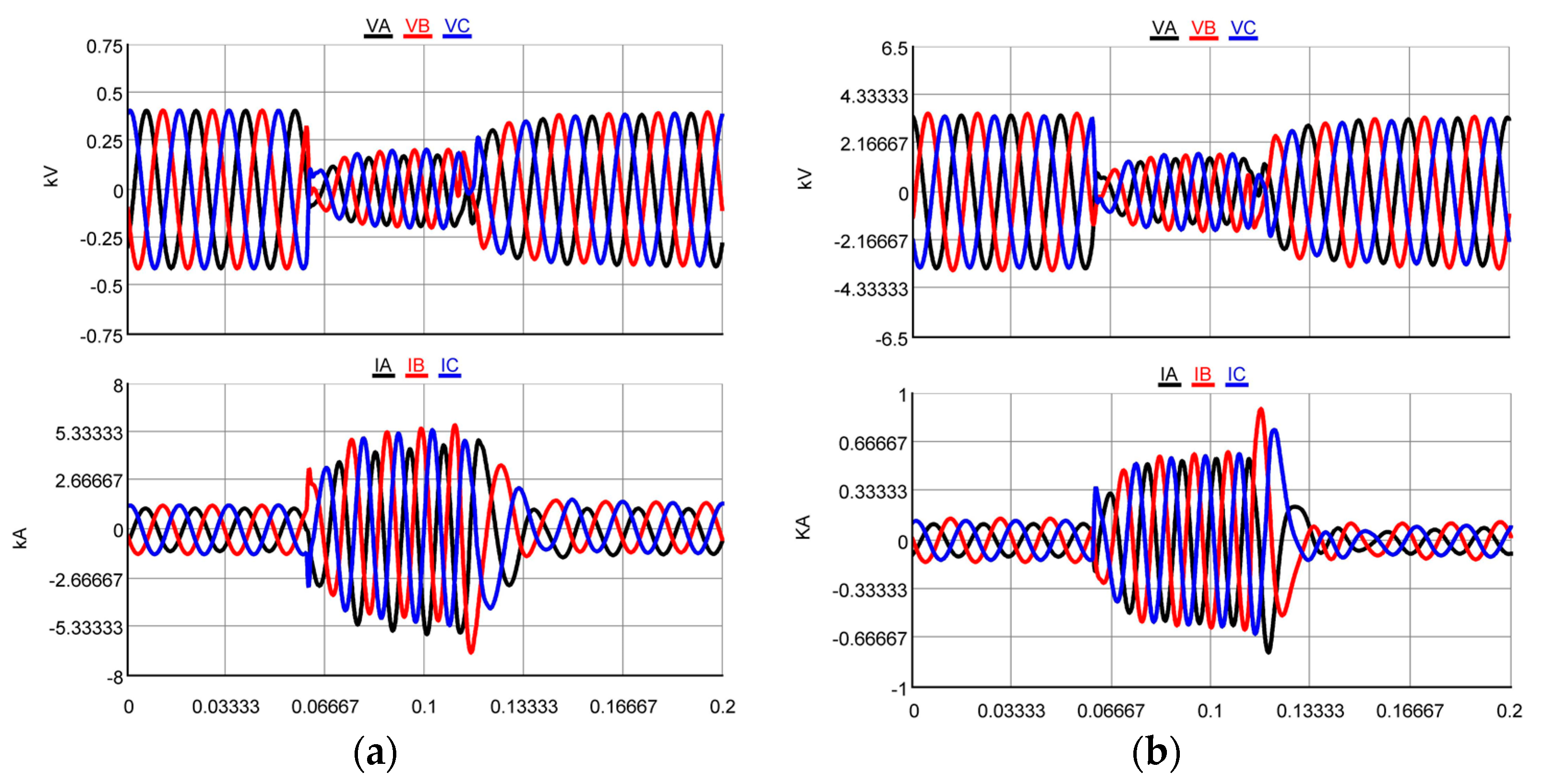
3.2. Impact of Fault Locations in the Transmission System on Solar PV Operation

In this case, the impact of fault locations in the transmission system on the operation of solar PVs in the distribution system is investigated. To this end, another fault with the same fault occurring and clearing time of the fault transpired at bus 6 is applied at bus 7 in the transmission system. Still, four types of faults at bus 7, including a three-phase fault, a single line-to-ground fault, a line-to-line fault, and a double line-to-ground fault, are considered. Following different types of faults at bus 7, the voltage and current of each solar PV bus are observed to analyze the responses of the five solar PVs in the distribution system. According to the previous analysis, it is known that when the fault is applied at bus 6, the three-phase fault has the most severe impact on the solar PV operation. For comparison, Figure 12 shows the voltage and current responses at solar PV buses 634 and 680 under the three-phase fault at bus 7 in the transmission system.

By comparing Figure 12 with Figure 8, it can be seen that when the fault location is moved far from the distributed solar PVs from bus 6 to bus 7 in the transmission system, the same fault has a less severe impact on solar PV operation. Since bus 7 is further than bus 6 in the transmission system for all solar PVs in the distribution system, the maximum transient voltage and current at bus 634 (or bus 680) following the three-phase fault at bus 7 is smaller than those at bus 634 (or bus 680) following the three-phase fault at bus 6. For example, the maximum transient voltage and current at bus 680 resulting from the fault at bus 7 is less than 1.0 p.u. and 5.67 p.u., respectively, but those resulting from the fault at bus 6 are 1.75 p.u. and 17 p.u. Thus, when the transmission-level fault location is closer to the solar PV buses, it has a substantial influence on solar PV operation in the distribution system.

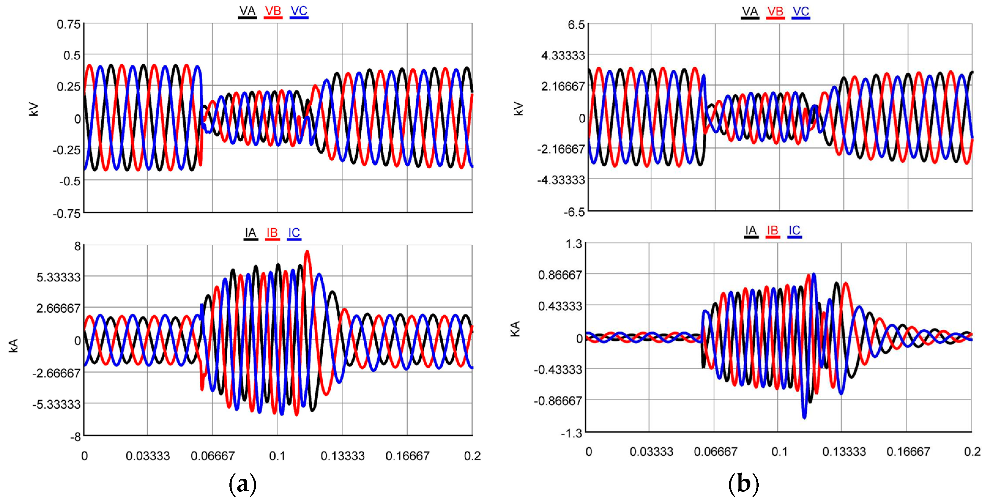
3.3. Impact of Solar Penetration Levels on Solar PV Operation under Transmission-Level Faults

Under the identified severe transmission-level fault type and location, the impact of solar penetration level on solar PV operation is further investigated. More specifically, the penetration level of the integrated solar PVs is changed by decreasing the irradiance level from 1000 W/m² to 750 W/m². Then, under the three-phase fault at bus 6 in the transmission system, Figure 13 shows the resulting voltage and current responses at solar PV bus 634 and bus 680 when solar PVs have the irradiance levels of 750 W/m².

By comparing Figure 13 with Figure 8, it can be seen that the severity of the impact of transmission-level disturbance on solar PV operation decreases with solar penetration level. As shown in Figure 13, both the maximum transient voltage and current decrease with the solar penetration level due to the irradiance decrease to 750 W/m² from 1000 W/m². For example, the maximum transient current is around 14.0 p.u. at solar PV bus 680 following the three-phase fault at bus 6 in the transmission system when all solar PVs in the distribution system have 750 W/m² solar irradiance, while the maximum current is increased to 17.0 p.u. at solar PV bus 680 resulting from the same fault when all solar PVs have 1000 W/m² solar irradiance. The maximum transient voltage in the case with 750 W/m² solar irradiance does not exceed the normal range but with 1000 W/m² solar irradiance has a peak of 1.75 p.u. for bus 680.

3.4. Impact of Loading Levels on Solar PV Operation under Transmission-Level Faults

Additionally, the impact of loading level on solar PV operation is investigated under the identified severe transmission-level fault type and location. In this case, the loading level is increased by four times its original loading level in the distribution system. Under the three-phase fault at bus 6 in the transmission system, the transient voltages and currents at the solar PV buses are investigated. For comparison, Figure 14 shows the resulting voltage and current responses at solar PV bus 634 and bus 680 after the loading is increased.

By comparing Figure 8 and Figure 14, it can be seen that the maximum transient voltage and current at bus 634 and bus 680 following the transmission-level fault at bus 6 are decreased with the increased loading. For example, before the loading level is increased in the distribution system following the transmission-level fault at bus 6, the maximum transient currents at solar PV bus 634 and bus 680 are approximately 3.0 p.u. and 17 p.u., respectively; after the loading is increased in the distribution system following the same transmission-level fault, the resulting maximum transient voltage and current decreases to 2.8 p.u. and 16.2 p.u. at bus 634 and bus 680.

3.5. Impact of Grid Strength on Solar PV Operation under Transmission-Level Faults with Different Solar Penetration Levels and Loading Levels

To understand the relationship between the previous investigation results with grid strength, the impact of grid strength on the solar operation is further analyzed in the system. To assess grid strength, the site-dependent short circuit ratio (SDSCR) [21] is used, which considers the interaction among solar PVs interconnected through the power network. The SDSCR at any point of interconnection (POI) i is calculated using the following Equation (1):

$$SDSC{R}_i=\frac{|V_{R,i}{|}^2}{\left(\left|P_{R,i}+{\displaystyle \sum _{j\in \mathit{R},j\ne i}{\omega }_{ij}{P}_{R,j}}\right|\right)|Z_{RR,ii}|}{\omega }_{ij}=\frac{Z_{RR,ij}}{Z_{RR,ii}}{\left(\frac{V_{R,i}}{V_{R,j}}\right)}^{*}$$

(1)

where R is the set of all POIs connected to IBRs; Z_RR,_ij is the (ith, jth) element in submatrix of bus impedance matrix that is only related to buses connected to IBRs; V_R,i is the voltage at POI i; P_R,i is the rated capacity or injected power from the IBR at POI i.

Based on the SDSCR defined in Equation (1), the grid strength at each POI of the solar PV in the distribution system in Figure 2 is evaluated.

Table 2. SDSCR values for solar PV buses in the distribution system.

Solar PV Buses	SDSCR Values
632	3.6346
634	3.3830
671	2.7768
675	3.0545
680	2.4765

lists the SDSCR values for the five POIs. If the SDSCR value is greater than 3, the grid is strong at the POI; if the SDSCR value is between 2 and 3, the grid is weak at the POI; if the SDSCR value is less than 2, the grid is very weak at the POI. Thus, it can be observed from Table 2 that buses 632, 634, and 675 are strong POIs since they have SDSCR values higher than 3. Bus 671 and 680 are the weak POIs as they have SDSCR values less than 3 but greater than 2.

4. Discussions

When comparing the evaluation results presented in Table 2 with the simulation results in Figure 8, Figure 9, Figure 10, Figure 11, Figure 12, Figure 13 and Figure 14, the following conclusions can be obtained:

By comparing Table 2 with Figure 8, Figure 9, Figure 10 and Figure 11, it is found that undesirable transient dynamics may be more likely to occur at weaker POIs under the same fault but different types. Moreover, the severity of the undesirable transient dynamics at the weaker POIs may increase with the fault type. Table 2 shows that bus 680 is weaker than bus 634. Comparing the maximum transient voltage and current at bus 634 with those at bus 680, it can be observed from Figure 8, Figure 9, Figure 10 and Figure 11 that the maximum transient voltage and current at bus 634 are smaller than those at bus 680 following the same transmission-level fault with the four different types. For example, when the single line-to-ground fault occurred in the transmission system, Figure 9 shows that the maximum transient current at bus 634 is approximately 2.4 p.u., but the maximum transient current at bus 680 is approximately 6.8 p.u. Moreover, when the fault type is changed into the severest three-phase fault, Figure 8 shows that the maximum transient voltage and current at bus 634 are approximately 1.72 p.u. and 3 p.u.; however, the maximum transient voltage and current at bus 680 are approximately 1.75 p.u. and 17 p.u.

By comparing Table 2 with Figure 12, it is also found that under the same three-phase fault but different locations, weak POIs are more likely to have undesirable transient dynamics. As shown in Table 2, bus 680 is weaker than bus 634. By comparing the maximum transient voltage and current at bus 634 with those at bus 680 in Figure 8 and Figure 12, it can be observed that when the three-phase fault is moved from bus 6 to bus 7 in the transmission system, the maximum current transient at bus 634 is decreased from 3 p.u. to 1.4 p.u.; the maximum current transient at bus 680 is decreased from 17 p.u. to 5.67 p.u. Additionally, even when the fault is far from the distribution system (at bus 7), weak bus 680 is still more likely to have an undesirable transient response than bus 634.

By comparing Table 2 with Figure 13, it is found that undesirable transient dynamics may be more likely to happen at weaker POIs under the increasing solar penetration level in the distribution system. Compared to bus 634, weak bus 680 has a more severe impact on solar PV operation following the same transmission-level fault. As shown in Figure 13, for bus 680, when the solar irradiance is 750 W/m², the maximum transient current is 14 p.u.; as shown in Figure 8, when solar irradiance is increased to 1000 W/m², the maximum transient current is 17 p.u. For bus 634, the maximum transient current is increased from about 2.2 p.u. to 3 p.u. when solar irradiance is increased from 750 W/m² to 1000 W/m².

By comparing Table 2 with Figure 14, it is found that increasing the loading level in the distribution system may decrease the risk of undesirable transient dynamics at weaker POIs following the transmission-level disturbance. As shown in Figure 8 and Figure 14, the severity of the impact of transmission-level disturbance on solar PV operation decreases with the increase in loading level in the distribution system. At the weak bus 680, this impact becomes relatively significant. Before increasing the loading level, the maximum transient current is 17 p.u. following the transmission-level fault at bus 6; the transient current is reduced to 16. 2 p.u. following the same transmission-level fault when the loading level is increased. This change can improve grid strength at bus 680 and thus reduce the risk of undesirable transient dynamics of solar PV at bus 680.

5. Conclusions

In this paper, a real-time RTDS-based simulation testbed was presented to explore the impacts of realistic transmission-level disturbances on solar PV operation in the distribution system. The testbed includes detailed modeling of components in the transmission and distribution systems along with the detailed PV models and its inverter controls to capture the accurate dynamic behaviors of solar PVs in response to the transmission-level disturbances. The testbed was used in this paper to investigate the transient responses from the solar PV inverters under different transmission-level disturbances regarding different fault types and locations, solar penetration levels, and loading levels. It is found that the grid strength at the POIs of solar PV inverters significantly affects the transient response from the solar PV inverters following the transmission-level disturbances. At weaker POIs, the transient response is more sensitive to the disturbances. Such sensitivity becomes more significant when the transmission-level disturbance is closer to the weak POIs or the disturbances become more severe. Additionally, the impact of the transmission-level disturbances on the solar PVs at the weak POIs exacerbate with the increasing solar penetration levels and loading levels. Thus, when an increasing number of IBRs are being integrated into the grid, it is important to study and develop new technologies for grid planning, operation, and protection in weak grid conditions to address the emerging issues of integrating the high penetration of solar PVs and other IBRs.

References

- North American Electric Reliability Corporation. 1200 MW Fault Induced Solar Photovoltaic Resource Interruption Disturbance Report; North American Electric Reliability Corporation: Atlanta, GA, USA, 2016. [Google Scholar]
- North American Electric Reliability Corporation. 900 MW Fault Induced Solar Photovoltaic Resource Interruption Disturbance Report; North American Electric Reliability Corporation: Atlanta, GA, USA, 2018. [Google Scholar]
- North American Electric Reliability Corporation. April and May 2018 Fault Induced Solar Photovoltaic Resource Interruption Disturbances Report: Southern California Events: 20 April 2018 and 11 May 2018; North American Electric Reliability Corporation: Atlanta, GA, USA, 2019. [Google Scholar]
- San Fernando Disturbance Southern California Event: 7 July 2020 Joint NERC and WECC Staff Report. Atlanta, GA, USA, 2020. Available online: https://www.nwpp.org/news/power-insights-podcast-episode-2-san-fernando-even (accessed on 25 June 2021).
- Kang, S.; Shin, H.; Jang, G.; Lee, B. Impact Analysis of Recovery Ramp Rate After Momentary Cessation in Inverter-based Distributed Generators on Power System Transient Stability. IET Gener. Transm. Distrib. 2020, 15, 24–33. [Google Scholar] [CrossRef]
- Pierre, B.J.; Elkhatib, M.E.; Hoke, A. Photovoltaic Inverter Momentary Cessation: Recovery Process is Key. In Proceedings of the 2019 IEEE 46th Photovoltaic Specialists Conference (PVSC), Chicago, IL, USA, 16–21 June 2019. [Google Scholar]
- Choi, N.; Park, B.; Cho, H.; Lee, B. Impact of Momentary Cessation Voltage Level in Inverter-Based Resources on Increasing the Short Circuit Current. Sustainability 2019, 11, 1153. [Google Scholar] [CrossRef] [Green Version]
- Zhu, S.; Piper, D.; Ramasubramanian, D.; Quint, R.; Isaacs, A.; Bauer, R. Modeling Inverter-Based Resources in Stability Studies. In Proceedings of the 2018 IEEE Power & Energy Society General Meeting (PESGM), Portland, OR, USA, 5–10 August 2018. [Google Scholar]
- Shin, H.; Jung, J.; Lee, B. Determining the Capacity Limit of Inverter-Based Distributed Generators in High-Generation Areas Considering Transient and Frequency Stability. IEEE Access 2020, 8, 34071–34079. [Google Scholar] [CrossRef]
- Mather, B.; Ding, F. Distribution-connected PV’s response to voltage sags at transmission-scale. In Proceedings of the 2016 IEEE 43rd Photovoltaic Specialists Conference (PVSC), Portland, OR, USA, 5–10 June 2016; pp. 2030–2035. [Google Scholar]
- Mather, B.; Aworo, O.; Bravo, R.; Piper, P.E.D. Laboratory Testing of a Utility-Scale PV Inverter’s Operational Response to Grid Disturbances. In Proceedings of the 2018 IEEE Power & Energy Society General Meeting (PESGM), Portland, OR, USA, 5–10 August 2018; pp. 1–5. [Google Scholar]
- Kenyon, R.W.; Mather, B.; Hodge, B.-M. Coupled Transmission and Distribution Simulations to Assess Distributed Generation Response to Power System Faults. Electr. Power Syst. Res. 2020, 189, 106746. [Google Scholar] [CrossRef]
- Shin, H.; Jung, J.; Oh, S.; Hur, K.; Iba, K.; Lee, B. Evaluating the Influence of Momentary Cessation Mode in Inverter-Based Distributed Generators on Power System Transient Stability. IEEE Trans. Power Syst. 2020, 35, 1618–1626. [Google Scholar] [CrossRef]
- Li, C.; Reinmuller, R. Fault Responses of Inverter-based Renewable Generation: On Fault Ride-Through and Momentary Cessation. In Proceedings of the 2018 IEEE Power & Energy Society General Meeting (PESGM), Portland, OR, USA, 5–10 August 2018. [Google Scholar]
- Pierre, B.J.; Elkhatib, M.E.; Hoke, A. PV Inverter Fault Response Including Momentary Cessation, Frequency-Watt, and Virtual Inertia. In Proceedings of the 2018 IEEE 7th World Conference on Photovoltaic Energy Conversion (WCPEC) (A Joint Conference of 45th IEEE PVSC, 28th PVSEC & 34th EU PVSEC), Waikoloa, HI, USA, 10–15 June 2018. [Google Scholar]
- RTDS Technologies Inc. Available online: https://www.rtds.com (accessed on 25 June 2021).
- Sauer, P.W.; Pai, M.A. Power System Dynamics And stability; Wiley Online Library: Hoboken, NJ, USA, 1998; Volume 101. [Google Scholar]
- Kersting, W.H. Distribution System Modeling and Analysis; CRC Press: Boca Raton, FL, USA, 2017. [Google Scholar]
- IEEE PES AMPS DSAS Test Feeder Working Group. Available online: https://site.ieee.org/pes-testfeeders/resources/ (accessed on 25 June 2021).
- Grainger, J.J.; Stevenson, W.D., Jr. Power System Analysis; McGrawHill: New York, NY, USA, 1994. [Google Scholar]
- Wu, D.; Li, G.; Javadi, M.; Malyscheff, A.M.; Hong, M.; Jiang, J.N. Assessing impact of renewable energy integration on system strength using site-dependent short circuit ratio. IEEE Trans. Sustain. Energy 2017, 9, 1072–1080. [Google Scholar] [CrossRef]