Algorithm for Implementation of Optimal Vector Combinations in Model Predictive Current Control of Six-Phase Induction Machines

Abstract

The development of new control techniques for multiphase induction machines (IMs) has become a point of great interest to exploit the advantages of these machines compared to three-phase topology, for example, the reduced phase currents and lower harmonic contents. One of the most analyzed techniques is the model-based predictive current control (MPC) with a finite control set. This technique presents high x–y currents because of the application of one switching state throughout the whole sampling period. Nevertheless, it is one of the most used due to its excellent dynamic response. To overcome the aforementioned drawbacks, new techniques called virtual vectors have been developed, but although there are several articles with experimental results, the algorithm for implementing the technique has not been appropriately described. This document provides a clear and detailed explanation for algorithm implementation of virtual vectors through two proposed variants VV4 and VV11, in a six-phase machine drive. The first entails lower computational cost and the second lower loss in the x–y plane. According to performance indicators such as the total harmonic distortion and the mean square error for both case studies, experimental tests were evaluated to determine the implementation’s behaviour.

1. Introduction

For decades, three-phase IM was used for most variable speed applications, and control techniques are widely developed. Still, in recent years, the strengths of the multiphase IM has encouraged their use and thus the development of new sophisticated control techniques to regulate their speed, flux, torque or current. Multiphase IM stands out from three-phase IM due to the following characteristics: an inherent ability for post-fault operation without additional hardware, lower stator current per phase for the same voltage and lower torque ripple [1,2,3,4]. On the other hand, implementing more complex control strategies and the need for careful regulation of secondary currents that appear in multiphase IM also entails a higher computational cost [5,6]. However, this fact can be addressed through more powerful digital controllers such as Digital Signal Processor (DSP).

In this sense, concerning model-based control techniques, there are numerous options with their advantages and disadvantages. Among them is the MPC with finite set control, is one of the most widely used [7,8,9,10,11]. This technique employs a cost function to select an optimal vector from the 64 available vectors, for a six-phase IM, and apply it during the sampling period. The cost function consists of a configurable weighting factor to prioritize current tracking or loss reduction in the x–y plane. This method has the disadvantage of high tracking error and considerable losses in the x–y plane since it uses a single vector [12,13,14]. This fact produces high harmonic content in the stator currents compared to other approaches that integrate modulation strategies in MPC to face this weakness [15].

An alternative to mitigate the x–y currents was proposed in [12], called virtual voltage vectors (VV). This method minimizes current losses by using a zero vector (ZV), a large vector (LV), and the corresponding medium-large collinear vector (MLV) at each sampling time ($T_s$) since in the x–y plane, these vectors are 180 degrees out of phase and tend to be eliminated. Thus, to obtain a zero voltage on average in the x–y plane, it is necessary to apply the vectors in a certain proportion of time, which means the LV is applied $0.73$ of $T_s$ and the MLV $0.27$ of $T_s$ [16]. This technique uses less computational resources because it analyzes only 12 vectors; however, combining the vectors decreases the scope, covering only $93\%$ of the LV module in the $\alpha$–$\beta$ plane.

Another MPC called M2PC based on space vector modulation (SVM), it uses a cost function to determine a pair of optimal LV at each $T_s$. The selected optimal LV and the ZV a combination is performed to represent the target voltage more accurately, cover $96\%$ of the entire $\alpha$–$\beta$ plane. This method allows to cover an area, therefore minimising the tracking error and naturally reducing the losses because the LV are mapped as the smallest in the x–y plane [17].

Recently, other MPC techniques have been developed, namely as NM2PC, which uses up to 4 active vectors at each $T_s$ and does not use the ZV. Employing a cost function, it selects up to 4 vectors, two LV and two medium vectors (MV) to reduce the losses in the x–y plane. It is essential to mention that in M2PC, the cost function implements a weighting factor between current tracking and x–y loss reduction, and to some extent, it is expected that the algorithm tends to use the zero vector to reduce losses, even if the current tracking decreases in the $\alpha$–$\beta$ plane, so the NM2PC presents an advantage by not using the ZV, but on the other hand, the tracking ability of the controller for small currents deteriorates [18]. Further, in [19], it was shown a direct relationship between the stability of modulated MPC and the values of sampling frequency and rotor speed for multiphase machines.

Although several works, as described above, have reported experimental implementations of MPC techniques for multiphase IM drives, few details have explained how to implement these techniques in DSP. In that sense, the main goal of this paper is to describe the implementation of optimal vectors combinations into MPC technique focused on two study situations called virtual vectors with four application times (VV4) and virtual vectors with 11 application times (VV11). In both cases, two active vectors with different duty cycles are used to effectively reduce the x–y currents and improve the current tracking capability using an asymmetrical six-phase IM. Experimental results are presented to contrast both study situations, comparing in terms of current tracking considering the mean square error (MSE) and total harmonic distortion (THD) of the stator currents, to analyze the performance of the system. The proposed method is tested at different operating points, considering transient and steady-state conditions.

The sections that compose the rest of this document are the following: the mathematical model of the six-phase IM is shown in Section 2, as well as the voltage source inverter (VSI) used. Section 3 presents the description of the classic MPC, which will be used for the proposed MPC design. Section 4 describes the optimal vectors combinations implementation into MPC using two VV case scenarios. Section 5 shows the experimental results of both proposed methods. Conclusions and special remarks are presented in the last section.

2. Six-Phase IM Mathematical Model

The system is composed of an asymmetrical six-phase IM and a six-phase VSI based on isolated gate bipolar transistors (IGBT) connected as shown in the electrical diagram in Figure 1. The stator phase voltages of the six-phase IM depend on the switching states and the dc-link voltage source ($V_{dc}$). In this regard, complementary signals are applied to each leg of the six-phase VSI, and thus it is possible to obtain $2^6=64$ different switching states. These states are represented by a six-dimensional vector $\left[S\right]=[S_a,S_d,S_b,S_e,S_c,S_f]$. Then, the stator phase voltages can be calculated from the ideal six-phase VSI model as shown below:

$$\left[\begin{array}{c}{v}_{as}\\ v_{ds}\\ v_{bs}\\ v_{es}\\ v_{cs}\\ v_{fs}\end{array}\right]=\frac{V_{dc}}{3}\left[\begin{array}{cccccc}2& 0& -1& 0& -1& 0\\ 0& 2& 0& -1& 0& -1\\ -1& 0& 2& 0& -1& 0\\ 0& -1& 0& 2& 0& -1\\ -1& 0& -1& 0& 2& 0\\ 0& -1& 0& -1& 0& 2\end{array}\right]\left[\begin{array}{c}{S}_a\\ S_d\\ S_b\\ S_e\\ S_c\\ S_f\end{array}\right]$$

(1)

It is possible to simplify the system model employing the vector space decomposition (VSD) technique. Making transformations through the amplitude invariant Clarke conversion matrix (C), in this way is easy to represent the six-dimensional space defined by the six phases ($a,d,b,e,c,f$) in three two-dimensional orthogonal planes in the stationary reference frame, $\alpha$–$\beta$, x–y, and $z_1$–$z_2$. The $\alpha$–$\beta$ plane is related to the torque and flux production. The x–y plane is linked to the copper losses, while the components projected in the $z_1$–$z_2$ plane are not examined due to the adopted topology (isolated neutral points). The transformation matrix is shown below:

$$C=\frac{1}{3}\left[\begin{array}{cccccc}1& \frac{\sqrt{3}}{2}& -\frac{1}{2}& -\frac{\sqrt{3}}{2}& -\frac{1}{2}& 0\\ 0& \frac{1}{2}& \frac{\sqrt{3}}{2}& \frac{1}{2}& -\frac{\sqrt{3}}{2}& -1\\ 1& -\frac{\sqrt{3}}{2}& -\frac{1}{2}& \frac{\sqrt{3}}{2}& -\frac{1}{2}& 0\\ 0& \frac{1}{2}& -\frac{\sqrt{3}}{2}& \frac{1}{2}& \frac{\sqrt{3}}{2}& -1\\ 1& 0& 1& 0& 1& 0\\ 0& 1& 0& 1& 0& 1\end{array}\right]$$

(2)

Hence, using the transformation matrix defined in (2) the stator phase voltages are converted into orthogonal planes through the following equation:

$$\left[\begin{array}{c}{v}_{\alpha s}\\ v_{\beta s}\\ v_{xs}\\ v_{ys}\\ v_{z1s}\\ v_{z2s}\end{array}\right]=C\left[\begin{array}{c}{v}_{as}\\ v_{ds}\\ v_{bs}\\ v_{es}\\ v_{cs}\\ v_{fs}\end{array}\right]$$

(3)

It must be noted that the 64 switching states can be projected simultaneously in both planes as shown in Figure 2, where 49 of them are different. Vectors can be classified into (LV), (MLV), (MV), and (SV), which are marked as red, green, blue, and light blue circles, respectively.

Furthermore, the mathematical model of the system by using the state-space representation is expressed as follows:

$${\stackrel{.}{X}}_{\left(t\right)}=A_{\left(t\right)}{X}_{\left(t\right)}+B_{\left(t\right)}{U}_{\left(t\right)}+H{n}_{p\left(t\right)}$$

(4)

defining $X_{\left(t\right)}$ as the state vector, formed by stator and rotor currents as shown in (5), $U_{\left(t\right)}$ as the input vector constituted by the stator voltages represented by (6), while $A_{\left(t\right)}$ and $B_{\left(t\right)}$ are the matrices that contain the electrical parameters of the six-phase IM expressed in (7) and (8), respectively. The Gaussian process noises ($n_{p\left(t\right)}$), and its corresponding noise weighting matrix (H), defined as the identity matrix, have been contemplated in the model.

$$\begin{array}{c}{X}_{\left(t\right)}={\left[x_1,\dots ,x_6\right]}^T={[i_{\alpha s},i_{\beta s},i_{xs},i_{ys},i_{\alpha r},i_{\beta r}]}^T\end{array}$$

(5)

$$\begin{array}{c}{U}_{\left(t\right)}={[u_1,\dots ,u_4]}^T={[u_{\alpha s},u_{\beta s},u_{xs},u_{ys}]}^T\end{array}$$

(6)

$$A_{\left(t\right)}=\left[\begin{array}{cccccc}{a}_{11}& a_{12}& 0& 0& a_{15}& a_{16}\\ a_{21}& a_{22}& 0& 0& a_{25}& a_{26}\\ 0& 0& a_{33}& 0& 0& 0\\ 0& 0& 0& a_{44}& 0& 0\\ a_{51}& a_{52}& 0& 0& a_{55}& a_{56}\\ a_{61}& a_{62}& 0& 0& a_{65}& a_{66}\end{array}\right]$$

(7)

$$B_{\left(t\right)}=\left[\begin{array}{cccc}{b}_{11}& 0& 0& 0\\ 0& b_{22}& 0& 0\\ 0& 0& b_{33}& 0\\ 0& 0& 0& b_{44}\\ b_{51}& 0& 0& 0\\ 0& b_{62}& 0& 0\end{array}\right]$$

(8)

where the coefficients are defined as:

$$\begin{array}{cccc}\hfill a_{11}& =a_{22}=-\frac{R_s{L}_r}{L_s{L}_r-L_m^2}\hfill & \hfill a_{12}& =-a_{21}=\frac{L_m^2{\omega }_r}{L_s{L}_r-L_m^2}\hfill \\ \hfill a_{15}& =a_{26}=\frac{R_r{L}_m}{L_s{L}_r-L_m^2}\hfill & \hfill a_{16}& =-a_{25}=\frac{L_m{L}_r{\omega }_r}{L_s{L}_r-L_m^2}\hfill \\ \hfill a_{33}& =a_{44}=-\frac{R_s}{L_{ls}}\hfill & \\ \hfill a_{51}& =a_{62}=\frac{R_s{L}_m}{L_s{L}_r-L_m^2}\hfill & \hfill a_{52}& =-a_{61}=-\frac{L_s{L}_m{\omega }_r}{L_s{L}_r-L_m^2}\hfill & \\ \hfill a_{55}& =a_{66}=-\frac{R_r{L}_s}{L_s{L}_r-L_m^2}\hfill & \hfill a_{56}& =-a_{65}=-\frac{L_r{L}_s{\omega }_r}{L_s{L}_r-L_m^2}\hfill \\ \hfill b_{11}& =b_{22}=\frac{L_r}{L_s{L}_r-L_m^2}\hfill & \hfill b_{33}& =b_{44}=\frac{1}{L_{ls}}\hfill \\ \hfill b_{51}& =b_{62}=-\frac{L_m}{L_s{L}_r-L_m^2}\hfill \end{array}$$

$L_s=L_{ls}+L_m$, $L_r=L_{lr}+L_m$, $R_s$, and $R_r$ being the electrical parameters of the six-phase IM.

The output vector, including zero-mean Gaussian measurement noises ($n_{m\left(t\right)}$) and uncorrelated process, in the model, is calculated as follows:

$$Y_{\left(t\right)}=\left[\begin{array}{cccccc}1& 0& 0& 0& 0& 0\\ 0& 1& 0& 0& 0& 0\\ 0& 0& 1& 0& 0& 0\\ 0& 0& 0& 1& 0& 0\end{array}\right]X_{\left(t\right)}+n_{m\left(t\right)}$$

(9)

Finally, the torque ($T_e$) and the load torque ($T_L$) of the six-phase IM are obtained using the following equations:

$$T_e=3P\left({\psi }_{\alpha s}{i}_{\beta s}-{\psi }_{\beta s}{i}_{\alpha s}\right)$$

(10)

$$J_i{\stackrel{.}{\omega }}_m+B_i{\omega }_m=\left(T_e-T_L\right)$$

(11)

$${\omega }_m=\frac{{\omega }_r}{P}$$

(12)

$J_i$, $B_i$, ${\omega }_m$, ${\omega }_r$, ${\psi }_{\alpha s}$, ${\psi }_{\beta s}$ and P, being the inertia coefficient, the friction coefficient, the rotor mechanical speed, the rotor electrical speed, the stator fluxes and the number of pole pairs, respectively.

3. Classic MPC

To implement the classic MPC in a DSP, the mathematical model of the system must be in a discrete version. For this purpose, a discretization technique derived from the forward-Euler equation is used to obtain the predictive model. Note that the predicted variables only depending on past values of the variables and not on present values. As a result, the predictive model is described as:

$${\widehat{X}}_{(k+1|k)}=X_{\left(k\right)}+f\left(X_{\left(k\right)},U_{\left(k\right)},{\omega }_{r\left(k\right)},T_s\right)$$

(13)

being k the actual sample.

3.1. Reduced Order Observer

Rotor currents can be estimated through the reduced-order observer. There are two well-known techniques, the Luenberger Observer (LO) and the Kalman Filter (KF) [20,21], the latter being the more optimal as it takes into account the noise input to the sensors, thus optimizing the gain of the observer. Therefore, the KF is designed and implemented in this document, increasing the accuracy of the predictions. The equations of the mathematical model of system state space can be defined as:

$$\begin{array}{cc}\hfill {\widehat{X}}_{(k+1|k)}& =A_{\left(k\right)}{X}_{\left(k\right)}+B_{\left(k\right)}{U}_{\left(k\right)}+H{n}_{p\left(k\right)}\hfill \end{array}$$

(14)

$$\begin{array}{cc}\hfill Y_{(k+1|k)}& =\left[\begin{array}{cccccc}1& 0& 0& 0& 0& 0\\ 0& 1& 0& 0& 0& 0\\ 0& 0& 1& 0& 0& 0\\ 0& 0& 0& 1& 0& 0\end{array}\right]X_{(k+1)}+n_{m(k+1)}\hfill \end{array}$$

(15)

where k represents the actual sample, $n_{p\left(k\right)}$ the process noise, and H the noise weight matrix.

The discretized matrices $A_{\left(k\right)}$ and $B_{\left(k\right)}$ are represented in (16) and (17) respectively. $A_{\left(k\right)}$ depends on the present amount of the rotor electrical speed and it must be actualized at every sampling period.

$$A_{\left(k\right)}=\left[\begin{array}{cccccc}{a}_{11\left(k\right)}& a_{12\left(k\right)}& 0& 0& a_{15\left(k\right)}& a_{16\left(k\right)}\\ a_{21\left(k\right)}& a_{22\left(k\right)}& 0& 0& a_{25\left(k\right)}& a_{26\left(k\right)}\\ 0& 0& a_{33\left(k\right)}& 0& 0& 0\\ 0& 0& 0& a_{44\left(k\right)}& 0& 0\\ a_{51\left(k\right)}& a_{52\left(k\right)}& 0& 0& a_{55\left(k\right)}& a_{56\left(k\right)}\\ a_{61\left(k\right)}& a_{62\left(k\right)}& 0& 0& a_{65\left(k\right)}& a_{66\left(k\right)}\end{array}\right]$$

(16)

$$B_{\left(k\right)}=\left[\begin{array}{cccc}{b}_{11\left(k\right)}& 0& 0& 0\\ 0& b_{22\left(k\right)}& 0& 0\\ 0& 0& b_{33\left(k\right)}& 0\\ 0& 0& 0& b_{44\left(k\right)}\\ b_{51\left(k\right)}& 0& 0& 0\\ 0& b_{62\left(k\right)}& 0& 0\end{array}\right]$$

(17)

The discretized matrix coefficients were included in the Appendix A.

3.2. Cost Function

The objective of the cost function is to obtain a numerical value that allows a decision to be made by prioritizing one or more variables. We can optimize, for instance, the switching losses, torque ripple, harmonic content, or tracking error of stator currents. The latter is usually the priority, so the current tracking error calculations are made in the $\alpha$–$\beta$ and x–y plane. The current tracking error between the reference ($i_{s(k+2)}^{*}$) and their predicted values (${\widehat{i}}_{s(k+2)}$) in the $\alpha$–$\beta$ and x–y planes is calculated as follows:

$$\begin{array}{cc}\hfill & J=\sqrt{{\left(e_{\alpha s}\right)}^2+{\left(e_{\beta s}\right)}^2+{\lambda }_{xy}[{\left(e_{xs}\right)}^2+{\left(e_{ys}\right)}^2]}\hfill \end{array}$$

(18)

where

$$\begin{array}{c}{e}_{\alpha s}=i_{\alpha s(k+2)}^{*}-{\widehat{i}}_{\alpha s(k+2)}\\ e_{\beta s}=i_{\beta s(k+2)}^{*}-{\widehat{i}}_{\beta s(k+2)}\\ e_{xs}=i_{xs(k+2)}^{*}-{\widehat{i}}_{xs(k+2)}\\ e_{ys}=i_{ys(k+2)}^{*}-{\widehat{i}}_{ys(k+2)}\end{array}$$

(19)

Note that a second-step ahead prediction is implemented to consider the delay compensation. This fact is produced by the comparable time between the computation of the control signal and the sampling period [22]. The tuning parameter (${\lambda }_{xy}$) expressed in (18) is usually considered in the control of the multiphase machines to provide greater weight to the $\alpha$–$\beta$ currents over the x–y currents.

4. Proposed Algorithm

This section aims to describe the algorithm implementation in a DSP based on Optimal Vector Combinations characteristics into MPC described in [12,13,16].

4.1. Case 1: VV4

The first MPC strategy to be discussed in this paper is called VV4. The described implementation algorithm is based on the virtual vector technique [12]. It uses two vectors per sampling time, a long vector and the nearest collinear medium-large vector, to obtain the target voltage. The Figure 3 exemplifies the selection of two vectors, LV and MLV, from the I-sector of the $\alpha$–$\beta$ plane. The advantage is taken of the fact that the LV and collinear MLV are 180 degrees out of phase in the x–y plane, and although they have different modulus as shown in Figure 2, they tend to subtract each other, thus decreasing the losses in this plane.

The VV4 technique adopts strategies that take into account the ratio of the modulus of LV and MLV to calculate their application times to obtain a zero average value in the x–y plane. Suitably, it is required to apply $73\%$ of the LV time and $27\%$ of the MLV time as described in [12]. The VV4 technique proposes a simple algorithm, based mainly on an interrupt and four conditional sequences, which divide the time of total application in four intervals, for which it is possible to apply $75\%$ of the time LV and $25\%$ MLV. This virtual vector is applied as follows:

$$VV4=d_{l}LV+d_{ml}MLV$$

(20)

where $d_l=0.75T_{sv}$ and $d_{ml}=0.25T_{sv}$.

On the other hand, in VV4, there is a decrease in the maximum final voltage that can be reached since it conditions the use of the LV and MLV vectors, obtaining a resulting vector of lower modulus.

The process for the implementation of VV4 is shown in Figure 4 and detailed below:

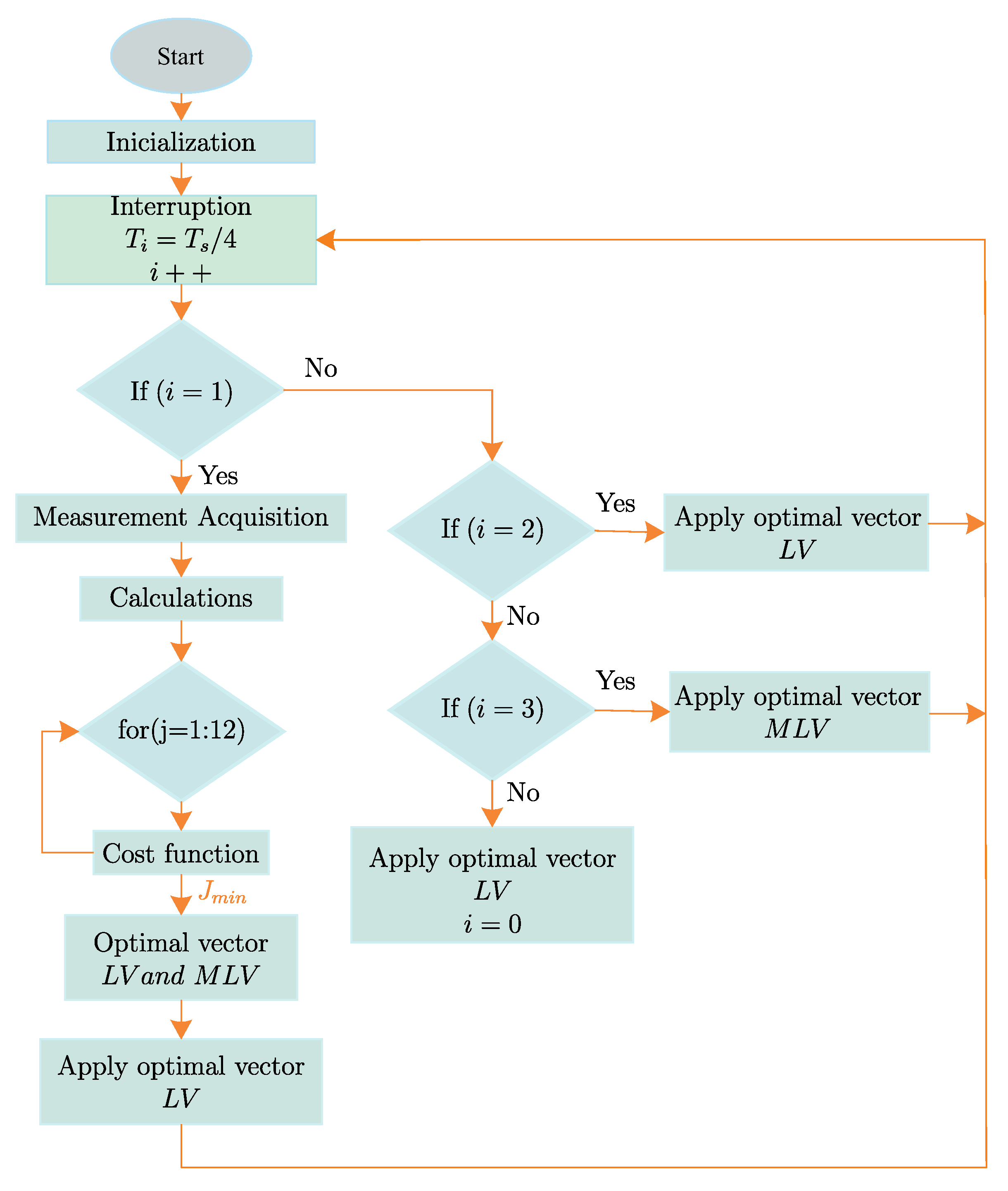
• Step 1: The algorithm starts with the variables initialization and calculation of the electrical parameters of IM.
• Step 2: The basic control technique, in this case the classical MPC, acquires measurements of the stator currents every sampling time ($T_s$). To implement the VV4 technique, the original sampling time ($T_s$) is increased by 4, hereafter referred to as ($T_{sv}$), consequently the sampling frequency is reduced by 4. On the other hand, an interrupt is used to control current readings, calculations and transforms, vector selection and application. The input period to the routines contained in this interrupt is every $T_{sv}$/4, and they are called interrupt time ($T_i$), so the interrupt is entered four times per sampling time.
• Step 3: In the first interval ($T_i$) of the sampling time ($i=1$), the measurements are considered to proceed to perform the transformations and calculations.
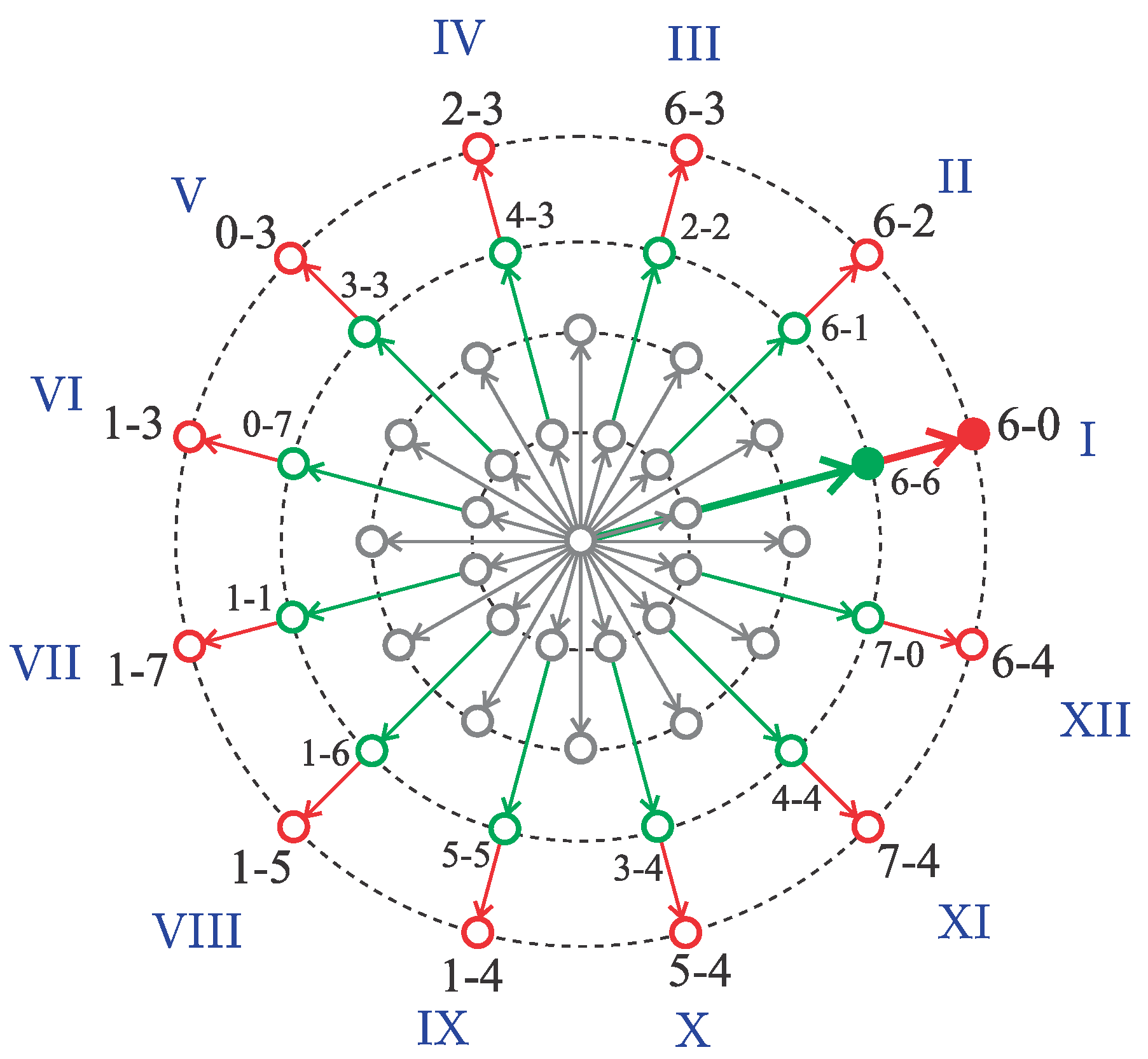
• Step 4: The 12 external vectors (LV) are evaluated using a cost function and the optimal vector is obtained. The MLV vector corresponding to the optimal LV is identified, and both will be applied during the sampling time.
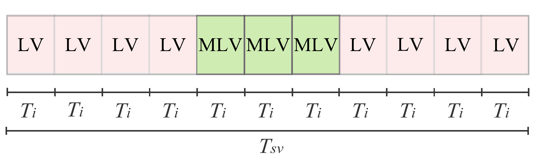
• Step 5: Only one vector is applied at each interrupt time, making use of conditional statements and a counter to identify the four interrupts in a sampling period. To reduce the losses in the x–y plane, the total application time of the active vectors is distributed between the LV and the MLV in a proportion of $75\%$ and $25\%$ respectively, so that the LV is applied three times and the MLV once. The final pattern of applied vectors is shown in Figure 5.

4.2. Case 2: VV11

The second case study is the technique called VV11, based on the MPC strategy with virtual vectors. Unlike VV4, in VV11 the LVand MLV are applied $73\%$ and $27\%$ of the time, so that the average loss in the x–y plane tends to zero. In order to achieve the latter, the sampling period is divided into 11 equal intervals, using an interrupt, conditional sequences, and a counter (i), so that $T_i$ = $T_{sv}/11$.

Similar to VV4, measurements are taken in the first interrupt of each sampling period ($i=1$), calculations, transformations are performed and optimal vectors are selected. Only one of them its applied in each $T_i$, in total, eight times the LV and three times the MLV are applied, resulting in approximately $72.73\%$ of $T_{sv}$ for LV and $27.27\%$ of $T_{sv}$ for MLV. The final applied vector pattern for VV11 is shown in Figure 6. This extra process implies higher computational costs compared to VV4, but it is closer to the appropriate proportion of application of the vectors LV and MLV.

5. Experimental Results

The case studies are implemented to analyze their performance by comparing them with each other through the experimental results collected in the six-phase IM bench.

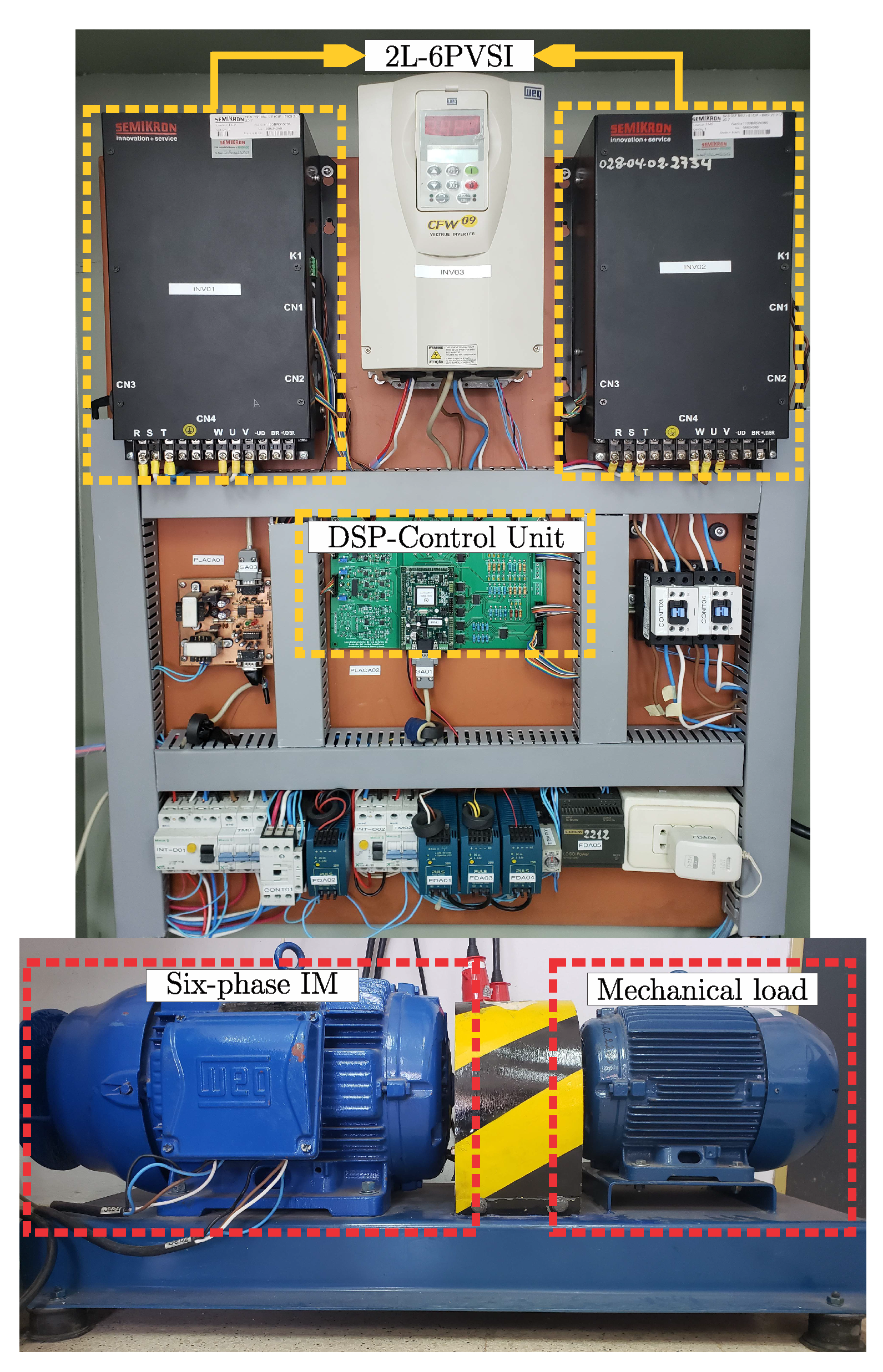
5.1. Six-Phase IM Test Bench Description

The control system is based on Six-Phase VSI, driven by a DSP (TMS320F28335 from Texas Instruments), with a Technosoft MCK28335 development environment. The IM parameters are shown in

Table 1. Electrical and mechanical parameters of the six-phase IM.

Parameter	Value	Parameter	Value
$R_r$	0.63 $\mathsf{\Omega }$	$L_s$	206.2 mH
$R_s$	0.62 $\mathsf{\Omega }$	P	3
$L_{ls}$	6.4 mH	$P_w$	15 kW
$L_{lr}$	3.5 mH	$J_i$	0.27 kg·m${}^2$
$L_m$	66.6 mH	$B_i$	0.012 kg·m${}^2$/s
$L_r$	203.3 mH	${\omega }_{r-nom}$	1000 rpm

determined by the tests described in [23,24].

The periodic measurements of the rotor currents and speed, necessary to perform the calculations and implement the control techniques, are made by a series of sensors. A 10,000 ppr encoder is used to obtain the mechanical speed of the motor.

A matching board is provided to amplify the signals coming from 4 LA 55-P sensors used to measure the stator currents. The digitalization is performed by means of a 16-bit A/D converter of the DSP. A dc-link is set to 325 V through a three-phase rectifier and the power grid with a step-down transformer. A mechanical brake pad was installed to simulate mechanical loading of approximately 120 Nm. A block diagram of the test bench is shown in Figure 7.

5.2. Figures of Merit

First, we tested experimentally VV4 and VV11 to analyze the performance under steady-state and transient conditions. The MSE between the reference and stator current measured in the $\alpha$–$\beta$ and x–y planes is obtained to compare current and loss tracking. On the other hand, the THD in the $\alpha$–$\beta$ plane is calculated to quantify the harmonic distortion obtained with both techniques. In this context, the MSE is defined as:

$$\mathrm{MSE}\left(i_{s\mathsf{\Phi }}\right)=\sqrt[]{\frac{1}{N}\sum _{k=1}^N{(i_{s\mathsf{\Phi }}\left[k\right]-i_{s\mathsf{\Phi }}^{*}\left[k\right])}^2}$$

(21)

where N is the number of samples, $i_{s\mathsf{\Phi }}^{*}$ the stator current reference, $i_{s\mathsf{\Phi }}$ the measured stator currents and $\mathsf{\Phi }\in$ $\{\alpha ,\beta ,x,y\}$. At the same time, THD is defined as:

$$\mathrm{THD}\left(i_s\right)=\sqrt[]{\frac{1}{i_{s1}^2}\sum _{j=2}^N{\left(i_{sj}\right)}^2}$$

(22)

where $i_{s1}$ is the fundamental stator currents and $i_{sj}$ is the harmonic stator currents.

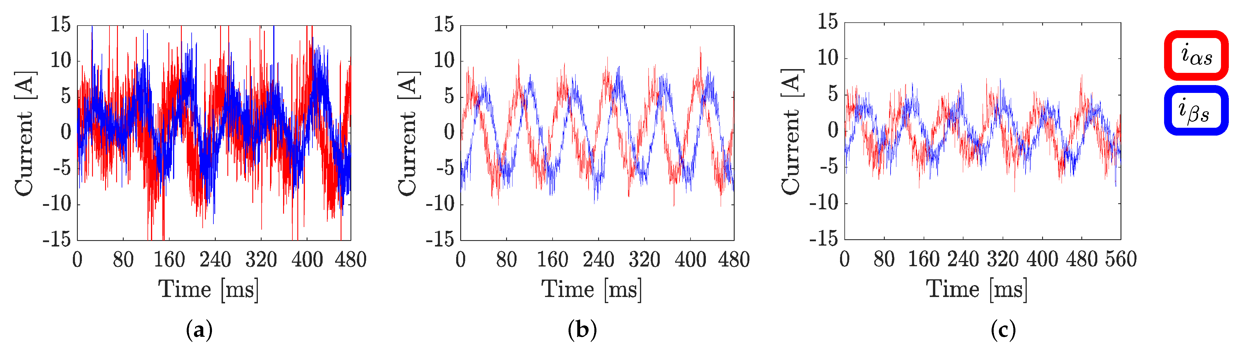
5.3. Steady-State Study

For the purpose of analyzing the performance of the x–y current, references are set to zero ($i_{xs}^{*}=i_{ys}^{*}=0$), and the d axis current ($i_{ds}^{*}=1.5$) has been considered for all cases.

For the VV4 and V11 technique, the sampling frequency is $2.5$ kHz. The tests are performed at mechanical speeds of 100 rpm to 600 rpm. The results obtained from VV4 and VV11 at the different speeds are shown in

Table 2. Performance indicators for the drive operating from 100 [rpm] to 600 [rpm] for VV4.

VV4       at       ${\mathit{f}}_{\mathit{s}}$ = 2.5 (kHz)
${\mathbf{\omega }}_{\mathit{m}}^{*}$	MSE${}_{\mathit{\alpha }}$	MSE${}_{\mathit{\beta }}$	MSE${}_{\mathit{x}}$	MSE${}_{\mathit{y}}$	THD${}_{\mathit{\alpha }}$
100	1.95	1.65	2.97	3.29	14.22
200	2.15	1.94	3.10	3.26	15.43
300	2.52	2.44	3.05	3.28	13.64
400	2.87	2.83	3.10	3.35	16.13
500	3.27	3.15	3.14	3.37	18.04
600	3.56	3.67	3.16	3.38	16.67

and

Table 3. Performance indicators for the drive operating from 100 [rpm] to 600 [rpm] for VV11.

VV11       at       ${\mathit{f}}_{\mathit{s}}$ = 2.5 (kHz)
${\mathit{\omega }}_{\mathit{m}}^{*}$	MSE${}_{\mathit{\alpha }}$	MSE${}_{\mathit{\beta }}$	MSE${}_{\mathit{x}}$	MSE${}_{\mathit{y}}$	THD${}_{\mathit{\alpha }}$
100	1.58	1.26	2.55	2.84	19.59
200	1.53	1.27	2.50	2.77	22.22
300	1.65	1.38	2.47	2.79	23.43
400	1.63	1.39	2.56	2.73	24.73
500	2.38	1.86	2.50	2.77	24.56
600	2.60	2.17	2.57	2.86	29.01

. At the same time, Figure 8 and Figure 9 show the stator currents tracking in $\alpha$–$\beta$ and x–y planes for classic MPC, VV4 and VV11 respectively. The operations were tested at a sampling frequency of $2.5$ kHz and a rotor speed of 200 rpm for the techniques.

The results show good current tracking in the $\alpha$–$\beta$ plane for both techniques, with a slight advantage for VV11, showing lower MSE values for all speeds. We can observe higher values for VV4 in terms of MSE in the x–y plane, corroborating the decrease in the resultant vector in the x–y plane also for all speeds. In terms of THD, it is observed that the VV11 technique leads to higher harmonic distortion.

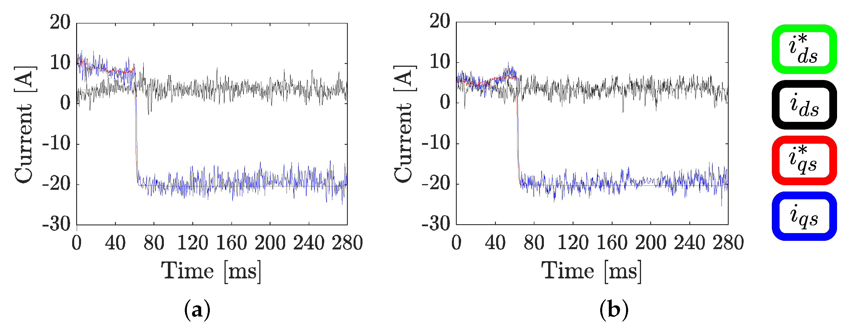
5.4. Transient Study

A step modification in the rotor speed is considered for a transient operation from 200 to $-200$ rpm (reversal condition) as shown in Figure 10. Additionally, Figure 11 presents a dynamic test (q current tracking), which reveals the transient operation of VV4 (a) and VV11 (b) for a step-change in the q current ($i_{qs}^{*}$). The dynamic performance is obtained through a reversal condition of the rotor speed (${\omega }_m^{*}$). The reaching time is approximately $0.5$ ms of both techniques, and the overshoot, for VV4 and VV11, are 10% and $12.5$%, respectively. Therefore, it can be noted that both control strategies show good speed tracking in reversal conditions; however, in terms of $i_{qs}$ current tracking, VV4 is slightly better than VV11.

6. Conclusions

The paper describes the implementation of two virtual vector modulation techniques applied to a 15 kW six-phase asymmetrical IM. Among the advantages of both techniques based on the same control strategy are: (a) reduced amount of switching, since only the change of state of the transistor pair of one VSI branch is required to switch from the MLV to the collinear LV; (b) combining LV and their corresponding MLV reduces the losses in the x–y plane. It can be seen in this work that as the combination of LV and MLV is closer to a ratio of $73\%$ and $27\%$ at each sampling time, the x–y currents and the MSE in the $\alpha$–$\beta$ plane are reduced, although these improvements are negligible compared to the $75\%$ and $25\%$ ratio used in VV4. On the other hand, the VV11, presents higher harmonic distortion and higher computational cost. These observations lead us to conclude that VV11 does not present a higher performance over VV4, so the best alternative in order to achieve good figures of merit and lower computational cost is VV4. It can be noted that due to the simple nature of the implemented controllers, they could be performed in any industrial application of a wide range of power and speed, being the computational cost the main reason to prefer VV4 over VV11.

References

1. Levi, E.; Bojoi, R.; Profumo, F.; Toliyat, H.; Williamson, S. Multiphase induction motor drives—A technology status review. IET Electr. Power Appl. 2007, 1, 489–516. [Google Scholar] [CrossRef] [Green Version]
2. Barrero, F.; Duran, M.J. Recent advances in the design, modeling, and control of multiphase machines—Part I. IEEE Trans. Ind. Electron. 2015, 63, 449–458. [Google Scholar] [CrossRef]
3. Duran, M.J.; Barrero, F. Recent advances in the design, modeling, and control of multiphase machines—Part II. IEEE Trans. Ind. Electron. 2015, 63, 459–468. [Google Scholar] [CrossRef]
4. Bermudez, M.; Gonzalez, I.; Barrero, F.; Guzman, H.; Kestelyn, X.; Duran, M.J. An experimental assessment of open-phase fault-tolerant virtual-vector-based direct torque control in five-phase induction motor drives. IEEE Trans. Power Electron. 2018, 33, 2774–2784. [Google Scholar] [CrossRef] [Green Version]
5. Kali, Y.; Ayala, M.; Rodas, J.; Saad, M.; Doval-Gandoy, J.; Gregor, R.; Benjelloun, K. Current control of a six-phase induction machine drive based on discrete-time sliding mode with time delay estimation. Energies 2019, 12, 170. [Google Scholar] [CrossRef] [Green Version]
6. Kali, Y.; Ayala, M.; Rodas, J.; Saad, M.; Doval-Gandoy, J.; Gregor, R.; Benjelloun, K. Time Delay Estimation based Discrete-Time Super-Twisting Current Control for a Six-Phase Induction Motor. IEEE Trans. Power Electron. 2020. [Google Scholar] [CrossRef]
7. Lim, C.S.; Levi, E.; Jones, M.; Rahim, N.A.; Hew, W.P. A comparative study of synchronous current control schemes based on FCS-MPC and PI-PWM for a two-motor three-phase drive. IEEE Trans. Ind. Electron. 2013, 61, 3867–3878. [Google Scholar] [CrossRef] [Green Version]
8. Lim, C.S.; Levi, E.; Jones, M.; Rahim, N.A.; Hew, W.P. FCS-MPC-based current control of a five-phase induction motor and its comparison with PI-PWM control. IEEE Tran. Ind. Electron. 2013, 61, 149–163. [Google Scholar] [CrossRef]
9. Levi, E.; Barrero, F.; Duran, M.J. Multiphase machines and drives-Revisited. IEEE Trans. Ind. Electron. 2015, 63, 429–432. [Google Scholar] [CrossRef] [Green Version]
10. Gonçalves, P.; Cruz, S.; Mendes, A. Finite control set model predictive control of six-phase asymmetrical machines—An overview. Energies 2019, 12, 4693. [Google Scholar] [CrossRef] [Green Version]
11. Pérez-Estévez, D.; Doval-Gandoy, J. A Model Predictive Current Controller With Improved Robustness Against Measurement Noise and Plant Model Variations. IEEE Open J. Ind. Appl. 2021, 2, 131–142. [Google Scholar] [CrossRef]
12. Gonzalez-Prieto, I.; Duran, M.J.; Aciego, J.J.; Martin, C.; Barrero, F. Model predictive control of six-phase induction motor drives using virtual voltage vectors. IEEE Trans. Ind. Electron. 2017, 65, 27–37. [Google Scholar] [CrossRef]
13. Aciego, J.J.; Prieto, I.G.; Duran, M.J. Model predictive control of six-phase induction motor drives using two virtual voltage vectors. IEEE J. Emerg. Sel. Top. Power Electron. 2018, 7, 321–330. [Google Scholar] [CrossRef]
14. Aciego, J.J.; Gonzalez-Prieto, I.; Duran, M.J.; Bermudez, M.; Salas-Biedma, P. Model predictive control based on dynamic voltage vectors for six-phase induction machines. IEEE J. Emerg. Sel. Top. Power Electron. 2020. [Google Scholar] [CrossRef]
15. González, O.; Ayala, M.; Romero, C.; Rodas, J.; Gregor, R.; Delorme, L.; González-Prieto, I.; Durán, M.J.; Rivera, M. Comparative Assessment of Model Predictive Current Control Strategies applied to Six-Phase Induction Machines. In Proceedings of the 2020 IEEE International Conference on Industrial Technology (ICIT), Buenos Aires, Argentina, 26–28 February 2020; pp. 1037–1043. [Google Scholar]
16. Durán, M.J.; Gonzalez-Prieto, I.; Gonzalez-Prieto, A. Large virtual voltage vectors for direct controllers in six-phase electric drives. Int. J. Electr. Power Energy Syst. 2021, 125, 106425. [Google Scholar] [CrossRef]
17. Gonzalez, O.; Ayala, M.; Doval-Gandoy, J.; Rodas, J.; Gregor, R.; Rivera, M. Predictive-Fixed Switching Current Control Strategy Applied to Six-Phase Induction Machine. Energies 2019, 12, 2294. [Google Scholar] [CrossRef] [Green Version]
18. Ayala, M.; Doval-Gandoy, J.; Rodas, J.; Gonzalez, O.; Gregor, R.; Rivera, M. A Novel Modulated Model Predictive Control Applied to Six-Phase Induction Motor Drives. IEEE Trans. Ind. Electron. 2020. [Google Scholar] [CrossRef]
19. Ayala, M.; Doval-Gandoy, J.; Gonzalez, O.; Rodas, J.; Gregor, R.; Rivera, M. Experimental Stability Study of Modulated Model Predictive Current Controllers Applied to Six-Phase Induction Motor Drives. IEEE Trans. Power Electron 2021, 1. [Google Scholar] [CrossRef]
20. Martin, C.; Arahal, M.R.; Barrero, F.; Durán, M.J. Five-phase induction motor rotor current observer for finite control set model predictive control of stator current. IEEE Trans. Ind. Electron. 2016, 63, 4527–4538. [Google Scholar] [CrossRef]
21. Martín, C.; Arahal, M.R.; Barrero, F.; Durán, M.J. Multiphase rotor current observers for current predictive control: A five-phase case study. Control Eng. Pract. 2016, 49, 101–111. [Google Scholar] [CrossRef]
22. Rodriguez, J.; Cortes, P. Predictive Control of Power Converters and Electrical Drives; John Wiley & Sons: Hoboken, NJ, USA, 2012; Volume 40. [Google Scholar]
23. Yepes, A.G.; Riveros, J.A.; Doval-Gandoy, J.; Barrero, F.; López, O.; Bogado, B.; Jones, M.; Levi, E. Parameter identification of multiphase induction machines with distributed windings Part 1: Sinusoidal excitation methods. IEEE Trans. Energy Conv. 2012, 27, 1056–1066. [Google Scholar] [CrossRef]
24. Riveros, J.A.; Yepes, A.G.; Barrero, F.; Doval-Gandoy, J.; Bogado, B.; Lopez, O.; Jones, M.; Levi, E. Parameter identification of multiphase induction machines with distributed windings Part 2: Time-domain techniques. IEEE Trans. Energy Conv. 2012, 27, 1067–1077. [Google Scholar] [CrossRef]
Figure 1. Six-phase IM fed by two level six-phase VSI.
Energies 14 03857 g001
Figure 2. Voltage vectors in the α β and xy planes for a six-phase IM drive.
Energies 14 03857 g002
Figure 3. Space sectors in the α β plane for MPC with VV.
Energies 14 03857 g003
Figure 4. Algorithm diagram for VV4 technique.
Energies 14 03857 g004
Figure 5. Timing diagram for VV4 technique.
Energies 14 03857 g005
Figure 6. Timing diagram for VV11 technique.
Energies 14 03857 g006
Figure 7. Test bench composed of the 2L-6PVSI, DSP unit control, six-phase IM and the mechanical load.
Energies 14 03857 g007
Figure 8. Performance of stator currents in α β plane for a rotor speed of 200 (rpm) at 2.5 (kHz) of sampling frequency: (a) classic MPC; (b) VV4; (c) VV11.
Energies 14 03857 g008
Figure 9. Performance of stator currents in xy plane for a rotor speed of 200 (rpm) at 2.5 (kHz) of sampling frequency: (a) classic MPC; (b) VV4; (c) VV11.
Energies 14 03857 g009
Figure 10. Reversal condition from 200 (rpm) to 200 (rpm) at 2.5 (kHz) of sampling frequency: (a) VV4; (b) VV11.
Energies 14 03857 g010
Figure 11. Transient response in q-axis of stator current for a rotor speed change from 200 (rpm) to 200 (rpm) at 2.5 (kHz) of sampling frequency: (a) VV4; (b) VV11.
Energies 14 03857 g011