Article

Experimental Study of the Space–Time Effect of a Double-Pipe Frozen Curtain Formation with Different Groundwater Velocities

1
State Key Laboratory of Mining Response and Disaster Prevention and Control in Deep Coal Mine, Huainan 232001, China
2
School of Civil Engineering and Architecture, Anhui University of Science and Technology, Huainan 232001, China
*
Author to whom correspondence should be addressed.
Energies 2021, 14(13), 3830; https://doi.org/10.3390/en14133830
Submission received: 17 May 2021 / Revised: 18 June 2021 / Accepted: 23 June 2021 / Published: 25 June 2021
(This article belongs to the Special Issue Advancements in Thermal and Energy Geotechnics)

Abstract

:
Groundwater velocity has significant effects on the formation of a frozen curtain during freezing. In order to study the influence of the velocity on a frozen curtain, a large physical model test platform was established for double-pipe freezing. Based on this platform, freezing tests for different velocities were carried out. Quartz sand was selected as a similar material. The freezing temperature of the saturated sand layer was found by analyzing the results of the nuclear magnetic resonance (NMR). Based on the study of the thermal physical properties of the sand layer, the freezing test results were analyzed, and the results showed that the flow led to the differential development of the temperature between the upstream and downstream sections of the freezing pipes. Moreover, the larger the velocity, the greater the difference. The flow prolonged the overlapping time of the frozen curtains. Additionally, the flow slowed down the development of the frozen curtain area and the frozen curtain thickness. The larger the flow velocity, the greater the inhibition of the flow on the development of the frozen curtain. The test results can provide more references for the design and construction of freezing engineering with flowing groundwater.

Graphical Abstract

1. Introduction

The artificial ground freezing (AGF) method is a common construction method that is widely used in mine and tunnel construction. This method reduces the temperature of a water-bearing stratum below the freezing point using an artificial cold source to form a frozen curtain. A frozen curtain with a certain strength has the function of supporting and blocking water, which provides the construction conditions for follow-up construction [1,2,3,4]. However, the existence of flowing groundwater will block the development of the frozen curtain and prolong the freezing overlapping time. When the velocity is large, the thickness of the frozen curtain will not meet the requirements, and it will even cause the frozen curtain to be difficult to close [5,6]. It has been found that the flowing groundwater will affect the distribution of a freezing temperature field and then affect the development of a frozen curtain [7]. Different velocities and flow directions will have different effects on freezing [8,9]. The further study of the evolution of a freezing temperature field and the development of a frozen curtain with different velocities is helpful for deepening the understanding of freezing construction, and it helps to reduce the freezing cost and to strengthen the freezing effect.
The impact of flowing groundwater on freezing has been studied by many scholars. Alzoubi et al. [10,11,12,13] systematically summarized and reviewed the theoretical basis, numerical models, and tests of the freezing method. Meanwhile, an experimental platform and a model based on the enthalpy-pore method were established to analyze the heat transfer of artificial frozen soil under the condition of high velocity. Vitel et al. [14,15] simulated the heat and mass transfer in the freezing process at a high permeability velocity, and they established a hydrothermal coupling model for freezing and then verified the model. Huang et al. [16] developed a THM model, and it could well simulate the thermal transfer and freezing expansion process of rock under freezing. Hu et al. [17] used a fully coupled model with consideration of the phase transition to analyze the effects of the water head difference, soil particle thermal conductivity, and pipe spacing on the overlapping time of a frozen curtain, and this model was applied in practical engineering. In terms of experiments, Zhou et al. [18] gave a detailed explanation of seepage velocity and groundwater velocity and conducted the model test. Wang et al. [19] carried out experimental research on ground freezing with liquid nitrogen under flowing water. Sudisman et al. [20], Shan et al. [21], and Yang et al. [22] carried out model tests of the vertical freezing of a single pipe, double-row pipes, and three pipes, respectively, and they studied the influence of groundwater velocity, freezing pipe spacing, freezing liquid temperature, and other factors. Wang et al. [23,24] conducted single pipe and double-pipe freezing tests to systematically study the influence of the velocity on the development of the freezing temperature. The above studies showed that the development of a frozen curtain was no longer uniform and symmetrical because of the effect of flowing groundwater, and the thicknesses of the frozen curtain at different positions were obviously different. In order to overcome this drawback, Marwan et al. [25] optimized a freezing scheme based on an ant colony optimization method combined with multiphase coupling theory to reduce costs. Huang et al. [26] optimized a non-uniform freezing curtain based on COMSOL and the Nelder–Mead simplex method, and the optimized layout significantly shortened the freezing time.
Through an analysis of the existing research, it can be found that the numerical simulation method and the model test method are mainly used to study the effect of flowing groundwater. Among them, the model test results can provide more guidance for theoretical analysis and a basis for numerical simulation. Although many scholars have carried out experimental research, the test sizes have often been small, which has limited the accuracy of the test results. At the same time, there is still a lack of detailed analysis regarding the influence of the velocities in the case of hydrothermal coupling. To further study the temporal and spatial evolution law of a freezing temperature field and the formation of a frozen curtain with the action of the flow, based on a large-scale controllable velocity physical model test platform, the experimental study of double-pipe freezing was carried out to determine the effect of the velocity. First, the thermal physical properties of a similar material were studied based on nuclear magnetic resonance (NMR) technology, and the design and analysis of the model test were guided based on the research results. Through the detailed analysis of the temporal and spatial evolution law of the temperature field, the distribution and development laws of the freezing temperature field for different velocities were mastered, and the formation of the frozen curtain was analyzed in depth combined with the distribution of the temperature field.

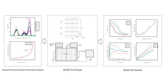
2. Experimental Study on Thermal Physical Properties of the Similar Materials

2.1. Selection of the Similar Materials

In practical engineering, flowing groundwater often exists in water-rich porous formations, such as sand and pebble formations. Considering this situation, standard quartz sand was selected as a similar material, which has uniform voids and clear properties. The sand layer composed of quartz sand can ensure the uniformity and stability of velocity in a freezing test. Most of the tests also used sand to form porous media materials [20,22]. The particle size of quartz sand is 0.5 ± 0.15 mm, and some physical properties are shown in Table 1.

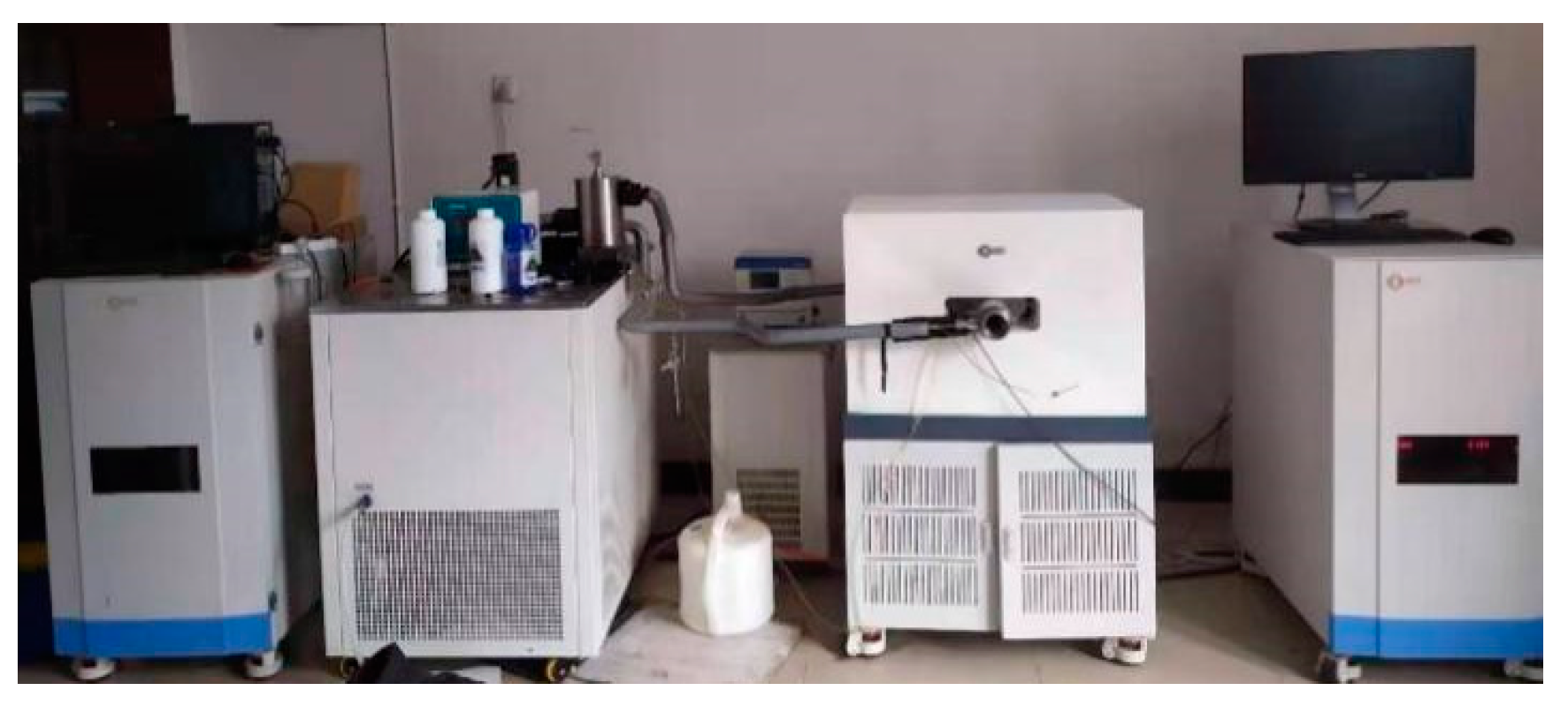
2.2. Test Method and Test Equipment

To better design and analyze the hydrothermal coupling model test, the freezing temperature of a similar material was analyzed. Freezing temperature is an important basis for judging the freezing state of a sand layer and the development of a freezing curtain, and it is also the basis of a model test. There are many methods used to measure the freezing temperature. In this research, the nuclear magnetic resonance (NMR) method was chosen [27]. The NMR method is fast and accurate, which is why it is widely used in frozen soil research. By analyzing the relationship between the energy level transition time T2 of a hydrogen atom in water and the signal intensity, the state and the content information of the water in the frozen sand layer could be obtained [28]. Through the analysis of the unfrozen water content in the sand layer, the freezing temperature was further obtained.
The test was based on low-field NMR technology, as shown in Figure 1. From left to right, the system mainly included a high pressure and low temperature control box, a constant temperature box, a magnetic field protection constant temperature box, a nuclear magnetic resonance instrument, and the test equipment. The main magnetic field intensity of the equipment was 0.5 T, the magnetic field uniformity was less than 20 ppm, and the RF power was 300 W.

2.3. Test Results

The sand with a moisture content of 19.9% (saturated) was prepared and studied in the temperature range of 0 °C to −18 °C. The relationship between the amplitude and the transverse relaxation time T2 is plotted as shown in Figure 2. In the figure, the area enclosed by the T2 curve and the coordinate axis is called the spectral crest area. The size of the spectral crest area is related to unfrozen water content, and the location of the spectral crest is related to pore size. It can be seen from Figure 2 that there were three crests in the T2 curve, which were Crest 1, Crest 2, and Crest 3, from left to right. According to the characteristics of the sand layer, it could be judged that Crest 1 corresponded to the bound water in the sand layer, and Crest 2 and Crest 3 corresponded to the free water in the sand layer. As shown in Figure 2, in the freezing process, the area of Crest 1, that is, the content of bound water in the sand sample, changed very little, while the content of free water decreased with the decrease of the temperature. In addition, the content of free water decreased rapidly from −0.5 °C to −2.5 °C. After −5 °C, the content of unfrozen water remained unchanged.
The relationship between the unfrozen water content and the temperature is shown in Figure 3. It can be more clearly seen from Figure 3 that when the temperature was lower than −0.5 °C, the unfrozen water content decreased rapidly as the temperature continued to decrease, and the unfrozen water content hardly changed after freezing to −5 °C. It can be judged from the figure that the freezing temperature of the similar materials was −0.5 °C. Furthermore, the power function was used to describe the relationship between temperature of the saturated sand layer and the unfrozen water content [29,30]. When the temperature was below the freezing temperature, the expression was:
θ = α (−T) β,
where θ is the unfrozen water content in the frozen soil, T is the temperature, and α and β are the two parameters that were obtained by fitting. The obtained fitting curve is shown in Figure 3. In the fitting, R2 > 0.94, and it could be seen that the power function fitting effect was good. For the frozen sand, α = 15.67, β = − 0.38.

3. Double-Pipe Freezing Model Test with Flowing Groundwater

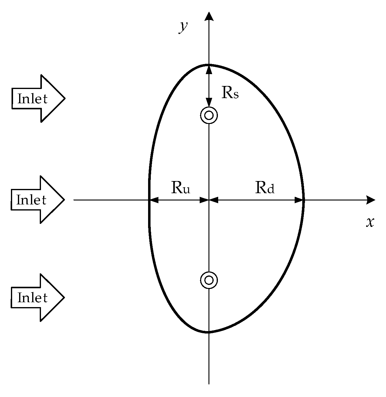
3.1. Model Test Design

The model test was designed based on the similarity theory. In order to better eliminate the boundary effect and reflect the temperature change in the real freezing project, the geometric similarity ratio Cl = 1/3 was selected. After the geometric similarity ratio was determined, other similarities were determined according to the similarity theory, as shown in Table 2. The size of the freezing core test area was determined to be 1500 mm × 2000 mm × 1000 mm. The test area was filled with quartz sand. The dimensions of each part of the box were the same as those in References [23,24].
In order to simulate the freezing under flowing groundwater accurately, a large-scale physical model test platform was assembled. The test system is shown in Figure 4. Based on the self-made test platform in References [23,24], the test system was further optimized by tamping the test area and strictly controlling the porosity of the sand layer. A high-precision flowmeter was used to strengthen the control of the flow. The effectiveness of the test system was confirmed by the pretest results. The whole setup of the test system mainly included a flowing system, freezing system, temperature measurement system, and test area. The flowing system was composed of a constant pressure water pump, high-precision flowmeter, and inlet and outlet pipelines. The aim of controlling the velocity was achieved by controlling the flow. The freezing system was composed of large freezing units. During freezing, low temperature alcohol was pumped into the freezing pipes. The alcohol entered from the inner pipe and flowed out from the outer pipe. After flowing back, the alcohol was cooled down to a certain temperature, and continued to be added into the circulation. The temperature measuring system was composed of a TDS 630 data acquisition instrument and copper-constantan thermocouples. The temperature measuring accuracy was 0.1 °C. To ensure the accuracy and reliability of temperature measurement, the temperature reduction test and ice-water mixture calibration test were carried out for each measuring point before the test. In the test, in order to reduce the influence of environmental temperature on the test results, the test box, pipeline, and so on were wrapped with insulation materials. At the same time, in order to better simulate the flow and prevent the water from flowing along the inner surface of the box, steel bars used for blocking water were set around the upstream cross section of the box. These measures further ensured the accuracy of the model test.

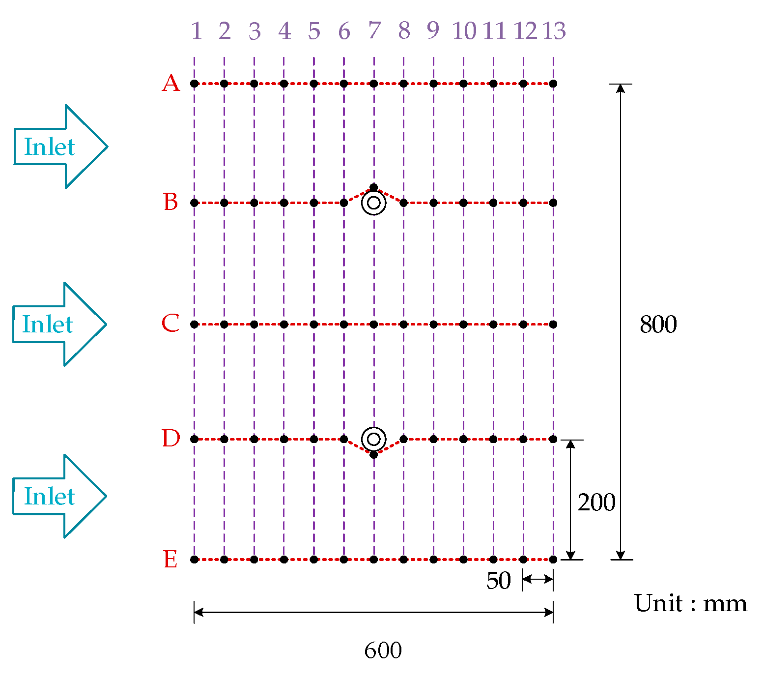
3.2. Test System and Measuring Point Layout

Without considering the change of temperature along the depth direction of the freezing pipe, the problem was simplified to a two-dimensional plane problem, and the measuring points were arranged on a horizontal plane. The plane of the measuring point was placed in the middle of the height of the inlet pipes and the outlet pipes of the flow, which could ensure the uniformity of the flow and reduce the influence of the boundary conditions. To measure and record the evolution law of the freezing temperature field as much as possible, five measuring axes, named A to E, were arranged around the two freezing pipes. The axes were arranged along the direction of flow. There were 13 temperature measurement points on each axis, of which points 1–6 were in the upstream of freezing pipes and points 8–13 were in the downstream of freezing pipes. All the measuring points were centered on the freezing pipes. The positions of the measuring axes and the freezing pipes are shown in Figure 5.

3.3. Test Scheme and Test Process

Based on the test platform, double-pipe freezing tests with different velocities were carried out. Considering the actual working conditions and existing experimental studies [19], four flow velocities (including no flow) were tested. The test scheme and the test process are shown in Figure 6. According to the similarity criterion of the cooling energy, the alcohol flow was determined to be 5 m3/h, the water temperature was kept at 15 °C, and the refrigerant temperature was −32 °C. For u = 3 m/d, 6 m/d, and 9 m/d, the water flows were 0.25 m3, 0.50 m3, and 0.75 m3, respectively. Here, the velocity u refers to the velocity of flowing water in the test, which was the same as that in the following introduction. In each group of tests, the temperature measurement system was the first to start, and the freezing system was the last to start. When the temperature at each measuring point was the same and the flow met the requirements, the test could be started. When the temperature at C7 on longer developed, the test was over.

4. Temporal and Spatial Evolution of Temperature Field in Double-Pipe Freezing

4.1. Change of Temperature with Freezing Time

The temporal and spatial evolutions of the temperature field for the above four velocities were further analyzed. It can be seen from Figure 5 that there were freezing pipes on the B axis and the D axis. Through the analysis of the B axis and the D axis, the development of the frozen curtain could be intuitively understood. The measuring point on the B axis was symmetrical about the freezing pipe, and the temperature at B7 was the temperature of the freezing pipe outer wall. It was found that at the beginning of freezing, the temperature at B7 was reduced rapidly to −29 °C and then remained stable. The temperatures at B3 (upstream) and B11 (downstream) were selected for analysis. The distance between the two measuring points and the freezing pipe was 200 mm. The temperature curves are shown in Figure 7.
Figure 7 shows the temperature variations at B3 and B11 with the freezing time for different velocities. Figure 7a shows the temperature reducing curve at B3 for four velocities. As shown in Figure 7a, the temperature at B3 was reduced with the freezing time. At the same freezing time, the larger the velocity, the higher the temperature at B3. Compared with the temperature reducing curves at u = 0 m/d and u = 3 m/d, the temperature at B3 at u = 6 m/d and u = 9 m/d began to reduce significantly later, and the temperature developed slowly in the initial stage of freezing. Taking the times from the beginning of the freezing to the temperature at B3 being reduced to 0 °C as an example, the times were 14.4 h, 15.7 h, 30.5 h, and 32.7 h for the four velocities. It can be found that the larger the velocity, the more time it took to reduce the temperature to 0 °C. In this test, in the positive temperature region, the temperature reducing rates at B3 were 0.53 °C/h, 0.39 °C/h, 0.26 °C/h, and 0.27 °C/h for the four velocities. Since the initial temperature of the sand layer at u = 9 m/d was higher than the other three groups of temperatures, it could be considered that the rate of the temperature reduction at B3 in the positive temperature zone decreased with the increase of the velocity. In the negative temperature zone (0 °C to the end of the test), the rate of the temperature reduction at B3 was stable near 0.20 °C/h, and the influence of the velocity was small. Figure 7b shows the temperature reduction curves of B11 with the freezing process for four velocities. It can be seen from the figure that the temperature variation change at B11 in the positive temperature zone was rapid when u = 6 m/d and 9 m/d. In the negative temperature zone, the temperature reduction rates at B11 were relatively stable for the four velocities, and the average rate was around 0.18 °C/h.
By comparing Figure 7a,b, it can be seen that the temperature in the upstream and downstream of the freezing pipe varied with freezing time. Under the condition of no flow, the temperatures at B3 and B11 had the same law of development, the temperature distribution was symmetrical, and the maximum temperature difference was 0.7 °C. When u = 3 m/d, the maximum temperature difference between B3 and B11 was 1 °C, and the temperature at B11 was lower than that at B3. When u = 6 m/d and 9 m/d, the developments of the temperature at B3 and B11 were obviously different. The temperature at B3 was reduced slowly in the early stage of freezing (positive temperature zone), and the temperature at B11 was reduced rapidly in the early stage of freezing. During the whole freezing process, the temperature at B11 was lower than that at B3. The analysis showed that the effect of the flow caused the difference of the temperature development between upstream and downstream. In the early stage of freezing, the flowing water absorbed the cold energy to reduce the temperature difference in the upstream points, and the low-temperature water after cooling accelerated the development of the temperature in the downstream, which made the downstream temperature develop faster than the upstream temperature. In the late stage of freezing, the frozen curtain blocked the flow of water, which made the upstream temperature begin to accelerate the reduction. The larger the velocity, the more obvious the effect of the flow. It can be seen from Figure 7 that at a large velocity, the temperature at B3 was reduced rapidly after 0 °C, and the temperature at B11 was reduced slowly after 0 °C.
The plane between the two freezing pipes was called the interface, and the C axis was on the interface. C7 was located between the two freezing pipes. The temperature variation at C7 is shown in Figure 8. It can be seen from the figure that the temperature at C7 was reduced with the freezing time, and the temperature reducing curves were relatively smooth near 0 °C for the four kinds of velocities. This was due to the heat released by the phase transformation, which partially offset the accumulation of cold energy and reduced the rate of temperature reduction. For the same freezing time, the larger the velocity, the higher the temperature at C7. In the positive temperature zone, the rates of the temperature reduction at C7 were 0.8 °C/h, 0.7 °C/h, 0.38 °C/h, and 0.34 °C/h. It can be found that the larger the velocity, the smaller the reducing rate at C7. In the negative temperature zone, the temperature reducing rates for different velocities were about 0.35 °C/h. B3, B11, and C7 were located at different positions of the freezing pipe, but they had the same distance from the freezing pipe. By comparing and analyzing the temperature development characteristics at the three positions, it could be determined that in the early freezing stage, the flow reduced the temperature reducing rate in the upstream of the freezing pipe, but the effect of the flow was weakened in the late freezing stage. Additionally, the downstream area was affected by the flow, and the temperature development was earlier than that upstream. Because of the superposition effect of the two freezing pipes, the reduction rate of the whole process was larger in the interface area, and the reduction rate in the positive temperature zone was larger than that in the negative temperature zone.

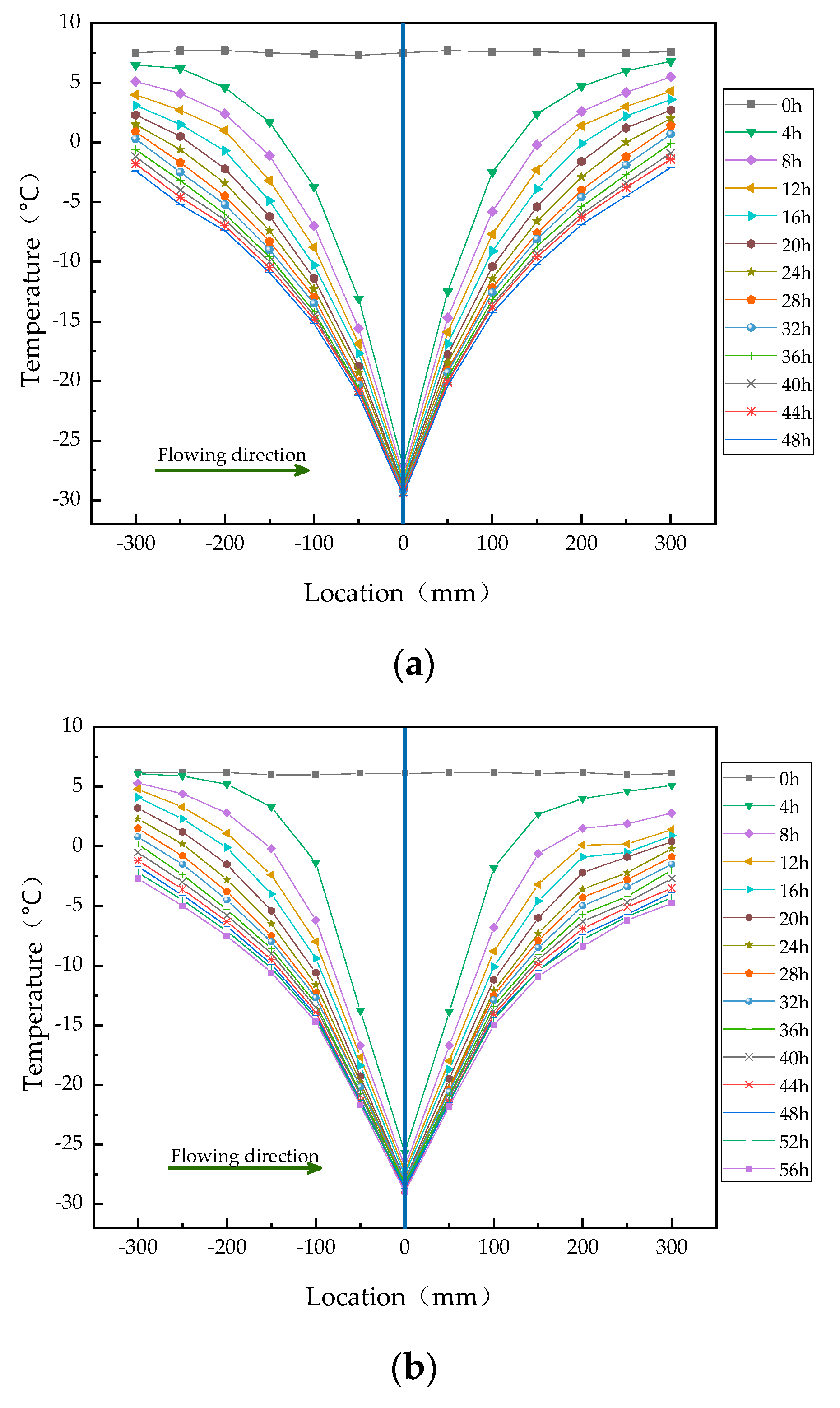
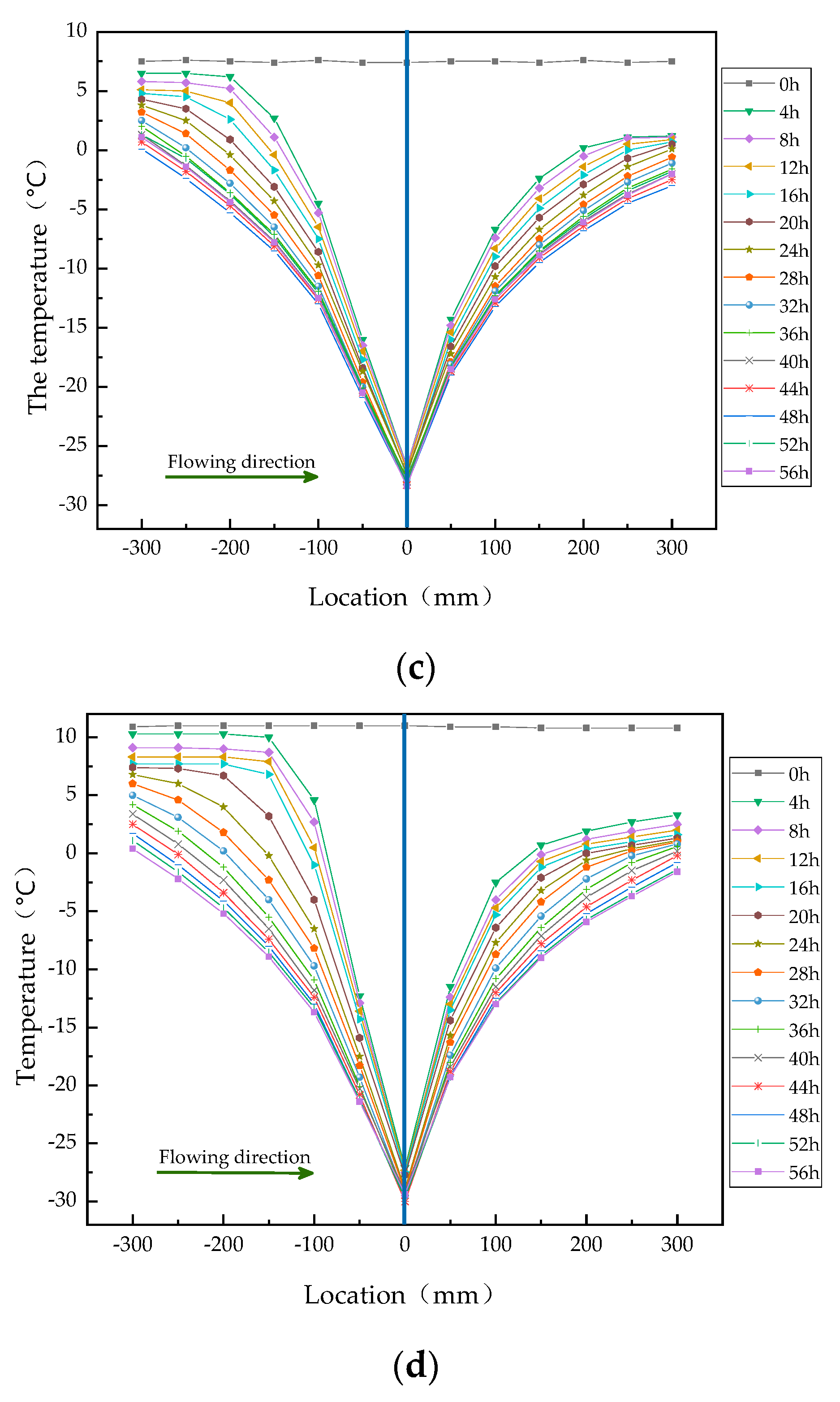
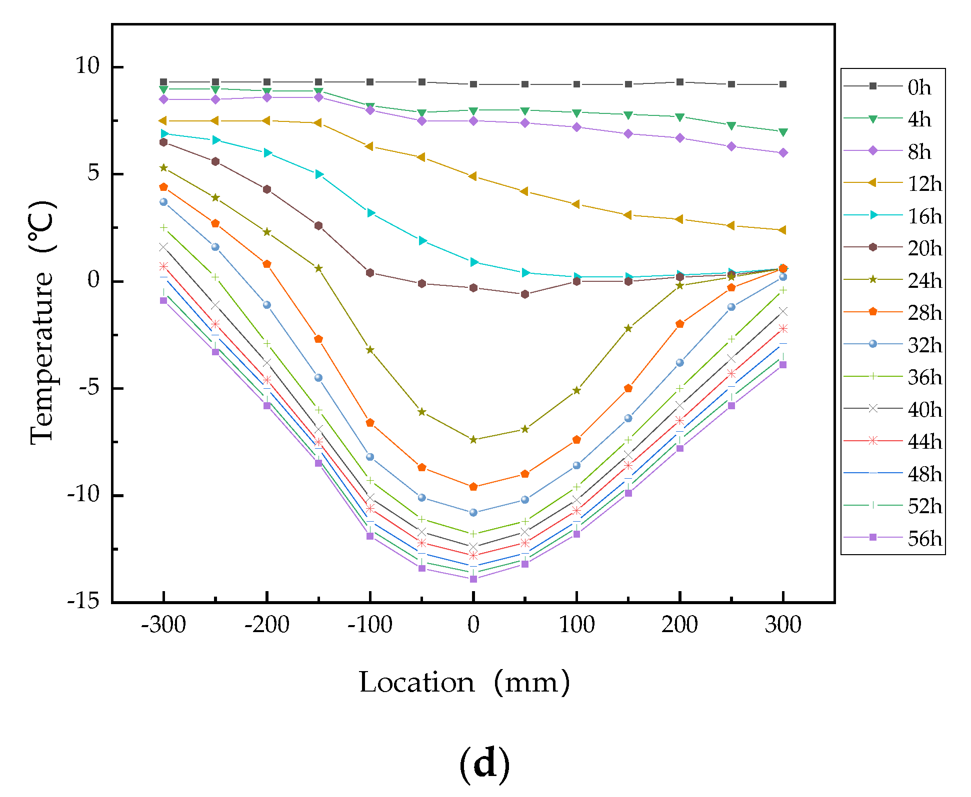
4.2. Spatial Distribution of Temperature Field

By analyzing the spatial distribution of the temperature field, the development of the freezing could be determined. Similarly, the measurement points on the B axis and the C axis were selected for analysis. The temperature distributions of measuring points on the B axis and the C axis are shown in Figure 9. It can be seen from Figure 9a that the temperature of the sand layer was basically the same before the beginning of the freezing. Once the freezing began, the temperature of each measuring point was reduced with the freezing pipe as the center. Additionally, the temperatures in the upstream and downstream of the freezing pipe reduced symmetrically. The closer to the freezing pipe, the faster the temperature reduced. At any given time, the temperatures in the upstream and downstream of the freezing pipe were the same. The temperature variations at the measuring points on the B axis in the presence of the flow are shown in Figure 9b, Figure 9c, and Figure 9d. The temperature in the upstream developed slowly, while the temperature in the downstream developed rapidly. Finally, the downstream temperature was lower than the upstream. The larger the velocity, the larger the temperature difference between symmetrical positions in the upstream and downstream. B1 and B13 which were the farthest away from the freezing pipe were selected. The variations of the temperature differences between two points for different velocities are shown in Figure 10.
It can be seen from Figure 10 that when u = 0 m/d, the differences between B1 and B13 were small and stable at about 0.3 °C. It was considered that these differences were symmetrically distributed. When there was flow, the temperature differences between the two points increased obviously. The larger the velocity, the larger the temperature difference between the two points. At the same velocity, the temperature difference first increased rapidly and then decreased slowly and gradually stabilized. When u = 3 m/d, 6 m/d, and 9 m/d, the maximum differences between the two points were 3.4 °C, 5.2 °C, and 7 °C, respectively. At the end of the test, the differences were stable at 2.1 °C, 3.1 °C, and 3.3 °C, respectively. It could be determined that the larger the velocity, the larger the temperature difference between upstream and downstream.
The temperature spatial distributions on the C axis for different velocities are shown in Figure 11. It can be seen from Figure 11 that when there was no flow, the temperatures in the upstream and downstream were symmetrical. The temperature at C7 was the lowest, but there was little difference with the temperature at C6 and C8. When there was flow, the downstream temperature was lower than the upstream temperature. At the same time, it can be found that the temperature reduction in the downstream was earlier than that in the upstream. For the four velocities, the temperatures at C6, C7, and C8 were almost the same when the temperatures reduced to 0 °C, which was due to the latent heat of the phase change. Comparing Figure 9 and Figure 11, it can be seen that the distribution law of temperature was similar. In these figures, the upstream temperature was higher than the downstream temperature, and the closer to the freezing pipe, the lower the temperature. Because there was a freezing pipe on the B axis, the influence of the phase change was relatively small. Figure 9 cannot show the characteristics of the phase change, while Figure 11 can. When comparing the changes of the temperatures on the C axis for different velocities, it can be found that with the increase of the velocity, the time required for the temperature to reduce was obviously longer. When the velocity was u = 0 m/d, the temperature at each point reduced obviously after freezing for 4 h. However, when u = 9 m/d, the temperature at each point reduced obviously after freezing for 20 h. The time taken for the temperatures at all measuring points on the C axis to reduce to 0 °C became longer and longer, at 28 h, 32 h, 48 h, and 52 h.

5. Analysis of the Formation Process of Frozen Curtain

5.1. Influence of the Flow on Overlapping Time of Frozen Curtain

The overlapping time of a frozen curtain is the key index in freezing design and construction, and it is a reference used to judge the feasibility of the scheme. The test results showed that the frozen curtains of the two freezing pipes developed independently after the beginning of the freezing. After freezing for a while, the frozen curtains interacted with each other, and then the frozen curtains tended to close. When there was no flow, the frozen curtains closed at C7 between the two freezing pipes. When there was flow, the close position was located at the downstream position between the two freezing pipes. The overlapping times of frozen curtains for different velocities in the test are shown in Figure 12. The overlapping time increased with the increase of the velocity. Compared with the case without flow, the overlapping times at 3 m/d, 6 m/d, and 9 m/d increased by 20%, 95%, and 180%, respectively. It can be seen from the analysis that the overlapping time increased less at 3 m/d, which indicated that the effect of the flow on the freezing was less when the velocity was small. When u = 6 m/d, the overlapping time increased by a large amount. Additionally, the overlapping time continued to increase with the increase of the velocity. Based on the relationship between the velocity and the overlapping time in this test, the influence of the flow had to be considered when the velocity was greater than 6 m/d.

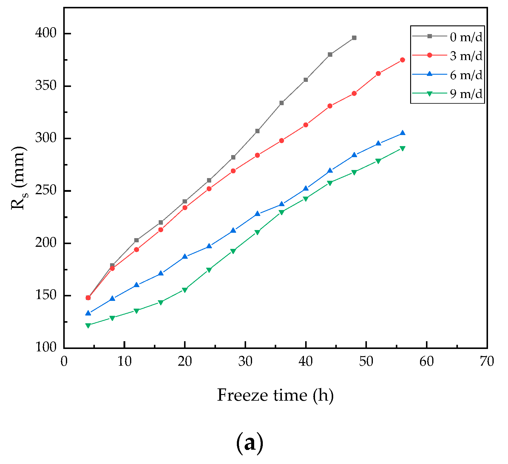
5.2. Influence of the Flow on the Development of Frozen Curtain Area

The frozen curtain developed with the freezing time. The development characteristics of the frozen curtain were analyzed by analyzing the area of the frozen curtain. According to the test results, the curves of the frozen curtain area are shown in Figure 13. To maintain the continuity of the curve, the area of the frozen curtain was the sum of the areas of the two frozen curtains before the intersection of the frozen curtains. According to the above analysis, the frozen curtains of the two freezing pipes were symmetrically distributed, so the frozen curtain area was twice that of a single freezing pipe before closing. It can be seen from Figure 13 that the area of the frozen curtain increased with the freezing time for the four velocities. In the range of the statistical time, the area of the frozen curtain had a linear positive correlation with the freezing time. The larger the velocity, the smaller the development rate of the frozen curtain area was. For the four velocities, the average development rates of the frozen curtain area in the whole freezing process were 16,662 mm2/h, 12,936 mm2/h, 10,072 mm2/h, and 8986 mm2/h.

5.3. Influence of the Flow on Shape Characteristics of the Frozen Curtain

Compared with the area of the frozen curtain, the shape characteristics information of the frozen curtain was also valuable, especially for weak surface monitoring. Three thicknesses were selected to describe the shape characteristics, including the side thickness of the frozen curtain Rs, the upstream thickness of the frozen curtain Ru, and the downstream thickness of the frozen curtain Rd. The positions of Ru, Rd, and Rs are shown in Figure 14.
Figure 15 shows the development curves of the frozen curtain thickness with freezing time for different velocities. As can be seen from Figure 15a, Rs began to appear and develop at the beginning of freezing, and Rs increased linearly with the freezing time. The larger the velocity, the slower the development of Rs. The flow had an inhibition effect on the side thickness of the frozen curtain Rs. Ru and Rd appeared after the frozen curtains closed. Ru continued to develop in the freezing process. Similarly, the larger the velocity, the slower the development of Ru. When the velocity was u = 0 m/d and 3 m/d, the relationship between Ru and the freezing time was linear. When the velocity was u = 6 m/d and 9 m/d, the development rate of Ru first increased and then decreased. That is to say, in the late stage of freezing, the high velocity had an obvious inhibitory effect on Ru. For the four kinds of velocities, Rd developed continuously; the larger the velocity, the smaller the development rate of Rd. The development rate of Rd first increased and then decreased at every velocity.
The average development rates of Rs, Ru, and Rd in the freezing process for different velocities are shown in Table 3. It can be seen from the table that Rs, Ru, and Rd were all restrained by the flow. The larger the velocity, the slower the development of the frozen curtain thickness. Comparing the development of the frozen curtain thickness for the same velocity, it can be found that when there was no flow, the development rates of the frozen curtain thickness in the upstream and downstream were the same. Compared with Ru and Rd, the development rate of Rs was slower. When there was flow, the development rate of Rd was the largest, and the development rate of Rs was the smallest. Compared with the development rates when u = 0 m/d, the development rates of Rs, Ru, and Rd at u = 9 m/d decreased by 42%, 32%, and 14%, respectively. It can be found that the flow had the greatest inhibition effect on Rs and the smallest inhibition effect on Ru.

6. Conclusions

In this research, in order to study the influence of the groundwater velocity on freezing, the freezing for a flow test platform was established, and double-pipe freezing model tests were carried out for four flowing velocities. The thermal physics properties of similar materials were tested with NMR. Combined with the analysis results of the freezing temperature of similar materials, the temperature field distribution and the formation process of the frozen curtain of freezing test were further analyzed. According to the analysis, the following conclusions were drawn:
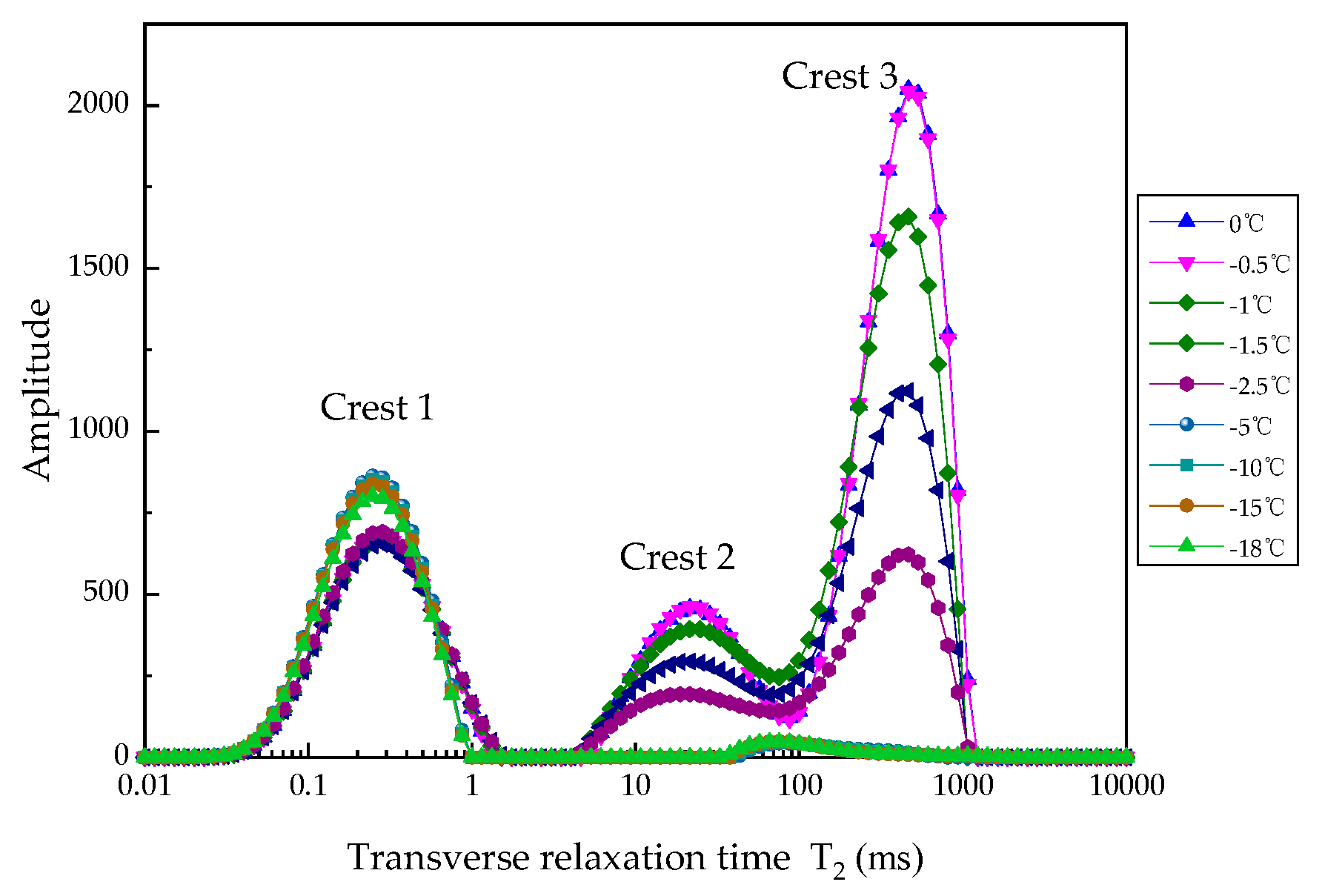
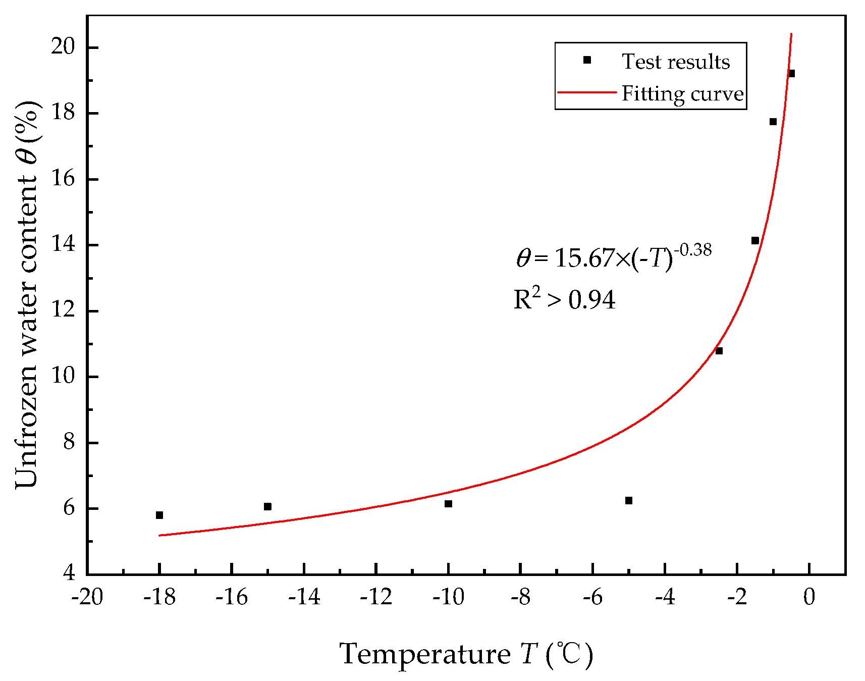
  • Based on NMR method, the saturated sand layer was studied, and it was found that the content of unfrozen water decreased rapidly between −0.5 °C and −2.5 °C, and the freezing temperature of the saturated sand was −0.5 °C. The relationship between the unfrozen water content and the temperature in the sand layer was further fitted, and it was found that the relationship between the unfrozen water content and the temperature satisfied the power function. For the saturated sand layer, the two parameters were α = 15.67 and β = −0.38.
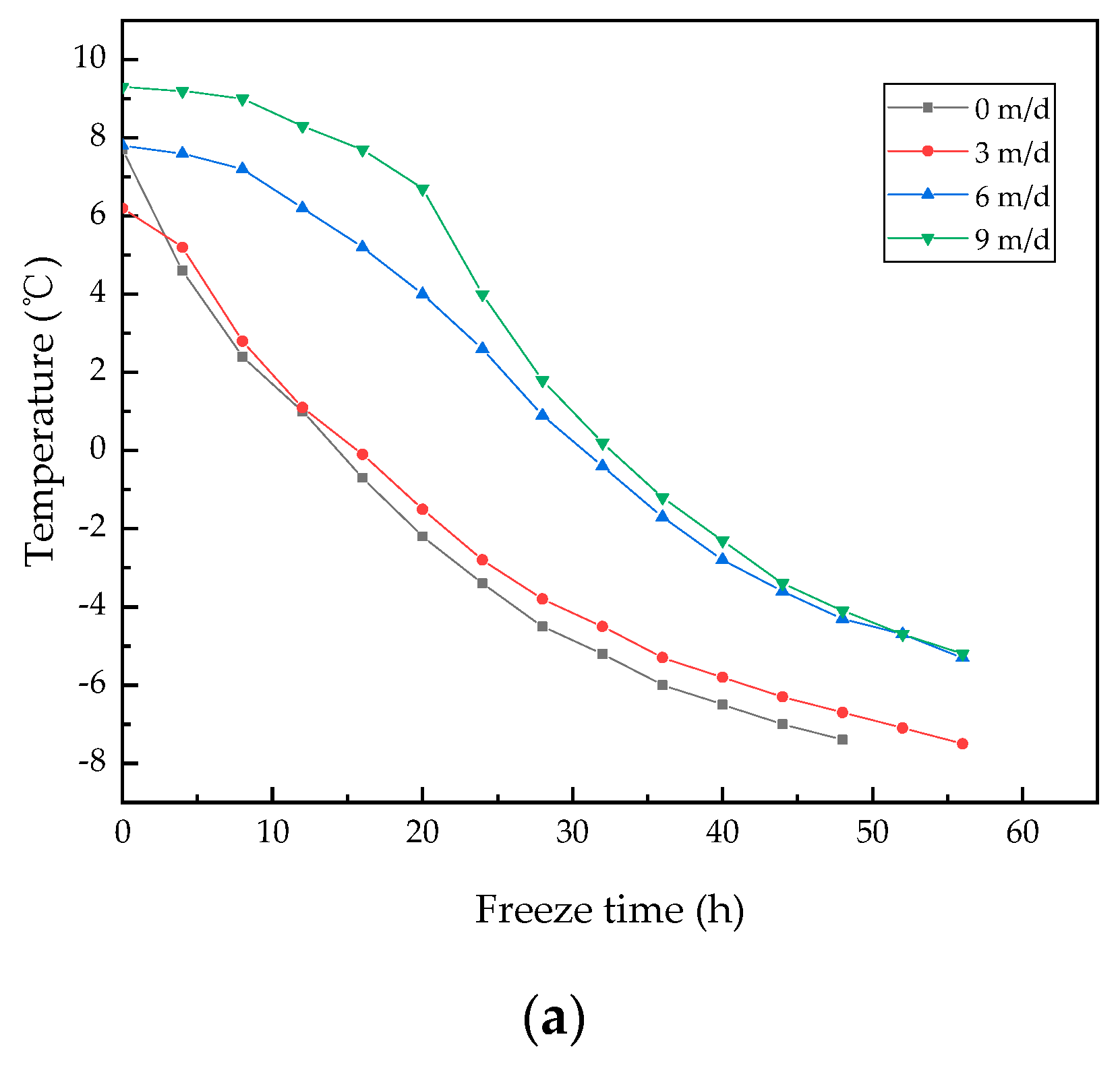
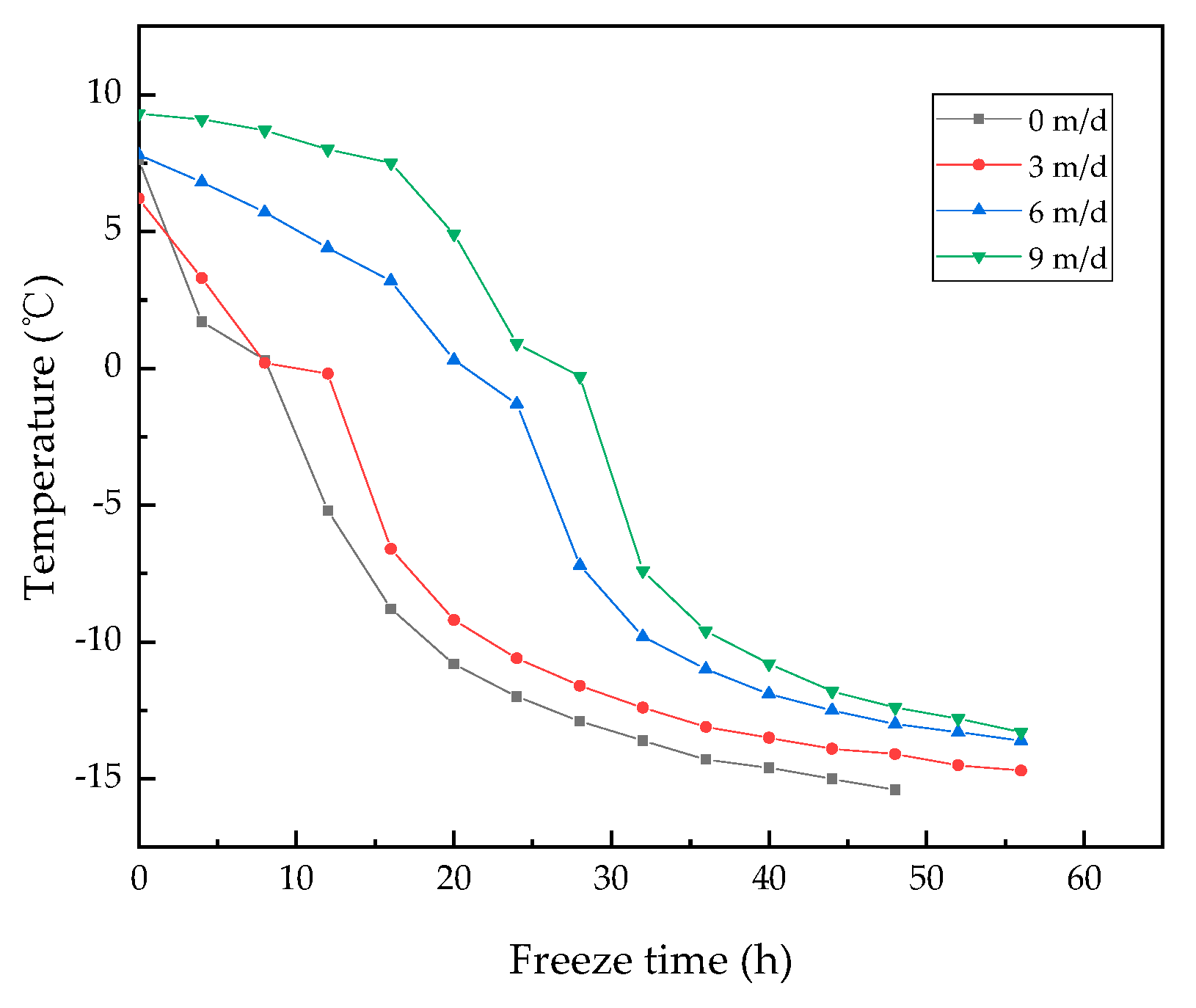
  • The flow led to the difference of the temperature evolution between upstream and downstream. During the process of freezing, in the positive temperature zone, the upstream temperature reducing rates at B3 were 0.53 °C/h, 0.39 °C/h, 0.26 °C/h, and 0.27 °C/h for the four velocities. In the negative temperature zone, the rates of the temperature reduction were stable near 0.20 °C/h. The rate of the temperature reduction in the upstream was larger than that in the downstream, and the flow had little effect on the reducing rate in the negative temperature zone. C7 was located between the two freezing pipes. Because of the superposition effect of the two freezing pipes, the reduction rate of the whole process was larger than that of B3 and B11. In the positive temperature zone, the rates of the temperature reduction at C7 were 0.8 °C/h, 0.7 °C/h, 0.38 °C/h, and 0.34 °C/h. In the negative temperature zone, the temperature reducing rates for different velocities were about 0.35 °C/h.
  • In the space, because of the flow, the downstream temperature was lower than the upstream temperature. Additionally, the larger the velocity, the larger the temperature difference. The temperature difference at the symmetrical points first increased, then decreased, and finally tended to be stable. When u = 3 m/d, 6 m/d, and 9 m/d, the maximum differences between B1 and B13 were 3.4 °C, 5.2 °C, and 7 °C, respectively. At the end of the test, the differences were stable at 2.1 °C, 3.1 °C, and 3.3 °C, respectively.
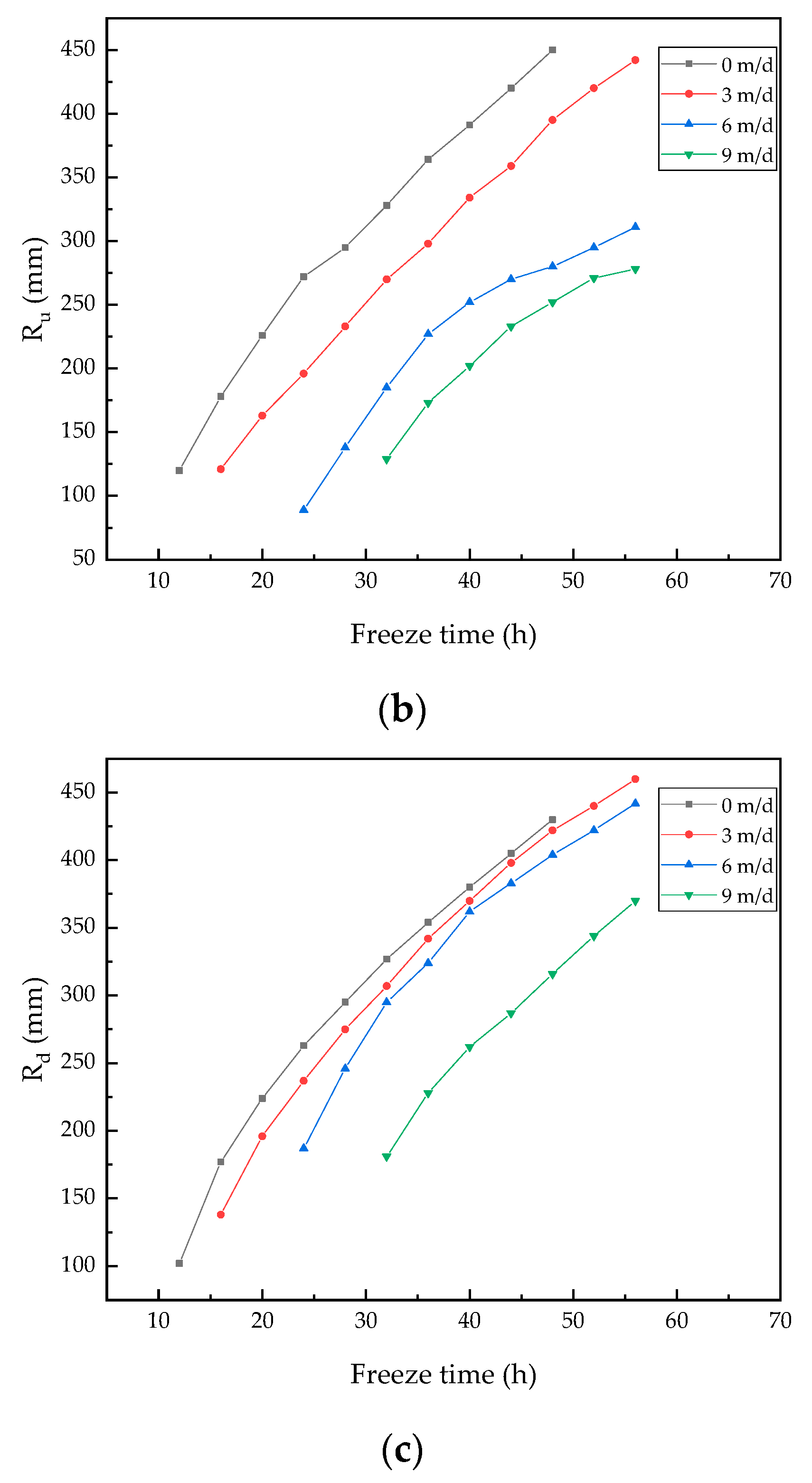
  • The flow prolonged the overlapping time of the frozen curtains. Compared with u = 0 m/d, the overlapping times at u = 3 m/d, 6 m/d, and 9 m/d were increased by 20%, 95%, and 180%, respectively. The development of the frozen curtain was inhibited by the flow. The larger the velocity, the slower the development of the frozen curtain. There was a linear positive correlation between the area of the frozen curtain and the freezing time. With the four velocities, the average development rates of the frozen curtain area in the whole freezing process were 16,662 mm2/h, 12,936 mm2/h, 10,072 mm2/h, and 8986 mm2/h. The statistical analysis of the frozen curtain thicknesses Rs, Ru, and Rd at the three locations showed that the developments of Rs, Ru, and Rd were all inhibited by the flow. The larger the velocity, the more obvious the inhibition. Compared with the development rates when u = 0 m/d, the development rates of Rs, Ru, and Rd at u = 9 m/d decreased by 42%, 32%, and 14%, respectively. The flow had the greatest inhibitory effect on the side thickness of the frozen curtain Rs, and it had the smallest inhibitory effect on the downstream thickness of the frozen curtain Rd.

Author Contributions

Conceptualization, C.R. and H.C.; methodology, B.W.; validation, S.S., X.J., and W.Z.; formal analysis, S.S.; investigation, Y.H.; resources, C.R.; data curation, S.S.; writing—original draft preparation, S.S.; writing—review and editing, S.S.; supervision, B.W.; project administration, W.Z.; funding acquisition, C.R. All authors have read and agreed to the published version of the manuscript.

Funding

This research was funded by the National Natural Science Foundation of China, grant number 51878005.

Data Availability Statement

The data used to support the findings of this study are available from the corresponding author upon request.

Conflicts of Interest

The authors declare that there are no conflicts of interest regarding the publication of this paper.

References

  1. Russo, G.; Corbo, A.; Cavuoto, F.; Autuori, S. Artificial ground freezing to excavate a tunnel in sandy soil. measurements and back analysis. Tunn. Undergr. Space Technol. 2015, 50, 226–238. [Google Scholar] [CrossRef]
  2. Wang, B.; Rong, C.X.; Cheng, H.; Yao, Z.S.; Cai, H.B. Research and application of the local differential freezing technology in deep alluvium. Adv. Civil. Eng. 2020, 2020, 9381468. [Google Scholar] [CrossRef]
  3. Gallardo, A.H.; Marui, A. The aftermath of the fukushima nuclear accident: Measures to contain groundwater contamination. Sci. Total Environ. 2016, 547, 261–268. [Google Scholar] [CrossRef]
  4. Huang, X.W.; Yao, Z.S.; Cai, H.B. An analytical heat-transfer model for coaxial borehole heat exchanger with segmented method. Energy Source Part A 2020, 10, 1851821. [Google Scholar] [CrossRef]
  5. Lin, J.; Cheng, H.; Cai, H.B.; Tang, B.; Cao, G.Y. Effect of seepage velocity on formation of shaft frozen curtain in loose aquifer. Adv. Mater Sci Eng. 2018, 2018, 2307157. [Google Scholar] [CrossRef] [Green Version]
  6. Li, Z.M.; Chen, J.; Sugimoto, M.; Ge, H.Y. Numerical simulation model of artificial ground freezing for tunneling under seepage flow conditions. Tunn. Undergr. Space Technol. 2019, 92, 103035. [Google Scholar] [CrossRef]
  7. Lao, L.Y.; Ji, Z.Q.; Huang, L.L.; Li, S.J. Research on the temperature field of a partially freezing sand barrier with groun-water seepage. Sci. Cold Arid Reg. 2017, 9, 280–288. [Google Scholar]
  8. Pimentel, E.; Sres, A.; Anagnostou, G. Large-scale laboratory tests on artificial ground freezing under seepage-flow conditions. Geotechnique 2012, 62, 227–241. [Google Scholar] [CrossRef]
  9. Wang, B.; Rong, C.X.; Lin, J.; Cheng, H.; Cai, H.B. Study on the formation law of the freezing temperature field of freezing shaft sinking under the action of large-flow-rate groundwater. Adv. Mater. Sci. Eng. 2019, 2019, 1670820. [Google Scholar] [CrossRef] [Green Version]
  10. Alzoubi, M.A.; Xu, M.H.; Hassani, F.P.; Poncet, S.; Sasmito, A.P. Artificial ground freezing: A Review of thermal and hydraulic aspects. Tunn. Under. Space Techno. 2020, 104, 1–18. [Google Scholar] [CrossRef]
  11. Alzoubi, M.A.; Nie-Rouquette, A.; Sasmito, A.P. Conjugate heat transfer in artificial ground freezing using enthalpy-porosity method: Experiments and model validation. Int. J. Heat Mass Trans. 2018, 126, 740–752. [Google Scholar] [CrossRef]
  12. Alzoubi, M.A.; Madiseh, A.; Hassani, F.P.; Sasmito, A.P. Heat transfer analysis in artificial ground freezing under high seepage: Validation and heatlines visualization. Int. J. Therm. Sci. 2019, 139, 232–245. [Google Scholar] [CrossRef]
  13. Alzoubi, M.A.; Sasmito, A.P.; Madiseh, A.; Hassani, F.P. Intermittent freezing concept for energy saving in artificial ground freezing systems. Energy Procedia. 2017, 142, 3920–3925. [Google Scholar] [CrossRef]
  14. Vitel, M.; Rouabhi, A.; Tijani, M.; Guérin, F. Thermo-hydraulic modeling of artificial ground freezing: Application to an underground mine in fractured sandstone. Comput. Geotech. 2016, 75, 80–92. [Google Scholar] [CrossRef]
  15. Vitel, M.; Rouabhi, A.; Tijani, M.; Guérin, F. Modeling heat and mass transfer during ground freezing subjected to high seepage velocities. Comput. Geotech. 2016, 73, 1–15. [Google Scholar] [CrossRef]
  16. Huang, S.B.; Liu, Q.S.; Cheng, A.P.; Liu, Y.Z.; Liu, G.F. A fully coupled thermo-hydro-mechanical model including the determination of coupling parameters for freezing rock. Int. J. Rock Mech. Min. 2018, 103, 205–214. [Google Scholar] [CrossRef]
  17. Hu, J.; Liu, Y.; Li, Y.P.; Yao, K. Artificial ground freezing in tunnelling through aquifer soil layers: A case study in Nanjing Metro Line 2. KSCE J. Civ. Eng. 2018, 22, 4136–4142. [Google Scholar] [CrossRef]
  18. Zhou, X.M.; Wang, M.S.; Zhang, X.Z. Model test research on the formation of freezing wall in seepage ground. J. China Coal Soc. 2005, 30, 196–201. (In Chinese) [Google Scholar]
  19. Wang, Z.H.; Zhu, X.R.; Zhu, G.X. The experimental researches on the ground freezing with liquid nitrogen under water flowing. J. Zhejiang Univ. 1998, 32, 534–540. (In Chinese) [Google Scholar]
  20. Sudisman, R.A.; Osada, M.; Yamabe, T. Experimental investigation on effects of water flow to freezing sand around vertically buried freezing pipe. J. Cold Reg. Eng. 2019, 33, 04019004. [Google Scholar] [CrossRef] [Green Version]
  21. Shan, R.L.; Liu, W.J.; Chai, G.J.; Xiao, S.C. Experimental study on influencing factors of characteristic index of local horizontal frozen body of double-row pipe under seepage. Adv. Mater. Sci. Eng. 2020, 2020, 8267692. [Google Scholar] [CrossRef] [Green Version]
  22. Yang, X.; Ji, Z.Q.; Zhang, P.; Qi, J.L. Model test and numerical simulation on the development of artificially freezing curtain in sandy layers. Transp. Geotech. 2019, 21, 100293–100376. [Google Scholar] [CrossRef]
  23. Wang, B.; Rong, C.X.; Cheng, H.; Cai, H.B.; Zhang, S.Q. Analytical solution of steady-state temperature field of single freezing pipe under action of seepage field. Adv. Civ. Eng. 2020, 2020, 5902184. [Google Scholar] [CrossRef]
  24. Wang, B.; Rong, C.X.; Cheng, H.; Cai, H.B.; Dong, Y.B.; Yang, F. Temporal and spatial evolution of temperature field of single freezing pipe in large velocity infiltration configuration. Cold Reg. Sci. Technol. 2020, 175, 5902184. [Google Scholar] [CrossRef]
  25. Marwan, A.; Zhou, M.M.; Abdelrehim, M.Z.; Meschke, G. Optimization of artificial ground freezing in tunneling in the presence of seepage flow. Comput. Geo. Tech. 2016, 75, 115–125. [Google Scholar] [CrossRef]
  26. Huang, S.B.; Guo, Y.L.; Liu, Y.Z.; Ke, L.H.; Liu, G.F.; Chen, C. Study on the influence of water flow on temperature around freeze pipes and its distribution optimization during artificial ground freezing. Appl. Therm. Eng. 2018, 135, 435–445. [Google Scholar] [CrossRef]
  27. Liu, H.W.; Zhang, X.F.; Leng, Y.F. Testing analysis on influencing factors of unfrozen water of frozen earth. North Commun. 2010, 9, 22–24. (In Chinese) [Google Scholar]
  28. Tan, L.; Wei, C.F.; Tian, H.H.; Zho, J.Z.; Wei, H.Z. Experimental study of unfrozen water content of frozen soils by low-field nuclear magnetic resonance. Rock Soil Mech. 2015, 36, 1566–1572. (In Chinese) [Google Scholar]
  29. Anderson, D.M.; Tice, A.R. Predicting unfrozen water contents in frozen soils from surface area measurements. Highw. Res. Rec. 1972, 393, 12–18. [Google Scholar]
  30. Lu, J.G.; Pei, W.S.; Zhang, X.Y.; Bi, J.; Zhao, T. Evaluation of calculation models for the unfrozen water content of freezing soils. J. Hydol. 2019, 575, 976–985. [Google Scholar] [CrossRef]
Figure 1. Low-field NMR system.
Energies 14 03830 g001
Figure 2. Variation of T2 distribution curve during the freezing of the saturated sand.
Energies 14 03830 g002
Figure 3. Relationship between unfrozen water content and temperature.
Energies 14 03830 g003
Figure 4. Test system diagram: (a) Schematic diagram of test system. 1, Constant temperature water tank; 2, constant pressure pump; 3, inlet flowmeter; 4, ball valve; 5, freezing machine; 6, alcohol flowmeter; 7, freezing pipes; 8, data acquisition instrument; 9, temperature measuring surface; 10, porous media; 11, buffer layer; 12, outlet flowmeter. (b) Photograph of the test system.
Energies 14 03830 g004
Figure 5. Layout of measuring points.
Energies 14 03830 g005
Figure 6. Test scheme and process.
Energies 14 03830 g006
Figure 7. Temperature variation at B3 and B11 under different velocity: (a) Temperature variation at B3; (b) temperature variation at B11.
Energies 14 03830 g007aEnergies 14 03830 g007b
Figure 8. Temperature variation at C7 with different velocities.
Energies 14 03830 g008
Figure 9. Spatial distributions of temperatures on the B axis at: (a) 0 m/d; (b) 3 m/d; (c) 6 m/d; (d) 9 m/d.
Energies 14 03830 g009aEnergies 14 03830 g009b
Figure 10. The temperature difference changes between B1 and B13 with the freezing time.
Energies 14 03830 g010
Figure 11. Spatial distribution of temperature on the C axis at: (a) 0 m/d; (b) 3 m/d; (c) 6 m/d; (d) 9 m/d.
Energies 14 03830 g011aEnergies 14 03830 g011b
Figure 12. The relationship between the velocities and the overlapping times.
Energies 14 03830 g012
Figure 13. The relationship between the freezing curtain area and the freezing time.
Energies 14 03830 g013
Figure 14. The positions ofRu, Rd,RS.
Energies 14 03830 g014
Figure 15. The development of the frozen curtain thickness at different locations for different velocities: (a) Rs; (b) Ru; (c) Rd.
Energies 14 03830 g015aEnergies 14 03830 g015b
Table 1. Physical properties of sand.
Dry Density (kg/m3)Saturated Density (kg/m3)PorositySaturated Moisture ContentPermeability Coefficient (m/s)Thermal Conductivity (W/mK)
161219420.3219.9%2.28 × 10−42.25
Table 2. Model similarity ratio.
Geometric Similarity Ratio ClTemperature Similarity Ratio CTTime Similarity Ratio CtVelocity Similarity Ratio Cu
1/311/93
Table 3. The development rate of frozen curtain thickness.
Flowing Velocity (m/d)0369
Development rate of Rs (mm/h)5.64.43.33.2
Development rate of Ru (mm/h)9.286.96.2
Development rate of Rd (mm/h)9.18.27.97.8
Publisher’s Note: MDPI stays neutral with regard to jurisdictional claims in published maps and institutional affiliations.

