Robust Operation of Hybrid Solar–Wind Power Plant with Battery Energy Storage System

Abstract

The intraday continuous electricity market (ICM) is a potential target market for the Dispatchable Hybrid Renewable solar–wind–battery energy storage system (BESS) power plant (DHRB). However, the uncertainty of the electricity price jeopardizes economic justification of BESS operation, an essential component of DHRB. Using the duality theory, this paper proposes a unilevel mixed-integer linear programming rolling-approach-based robust optimal scheduling tool for DHRB that keeps BESS operation optimal should the worst price scenario occur. It reflects BESS’s degradation as penalty factors and also integrates a BESS degradation model in the scheduling tool for better assessment of the available resources through the BESS’s lifetime. This tool aids the DHRB operator to decide the power offer to the ICM in such a way that the BESS’s operation remains optimal. A case study is carried out to demonstrate the application of the proposed tool. Both the long-term and short-term losses/benefits of utilizing this tool for scheduling DHRB in the ICM are investigated at various uncertainty levels. It is shown that there will be a risk of loss of income for the DHRB in the short-term due to increased nondispatchable energy. However, by limiting the use of BESS to only those settlement periods that are either certainly profitable or unavoidable, the lifetime of BESS can potentially be extended. Hence, this can result in more income by the DHRB power plant in the long-term.

1. Introduction

Dispatchability refers to the ability of the power system units (e.g., generator and demand) to change their power injection/draw within the announced operational limits, per the request of the system operator. Power system operation is centered around the key dispatchability feature of conventional generation units. Solar and wind power plants can potentially vary their output between zero and the maximum available power [1]. However, due to the intermittency of the available power (i.e., variable wind speed and solar irradiance), they are inherently nondispatchable, meaning there is no guarantee that the expected amount of power will be available on-demand, for a given period of time.

Power system penetration of renewables and in specific solar and wind generation has substantially increased worldwide. Realizing 100% renewables-based power systems is a hot topic under investigation [2]. Dispatchable renewable generation is the holy grail of 100% renewables-based power systems. It enables the participation of renewables in several electricity markets and potentially reduces the costs of reserve and flexibility associated with the integration of renewables.

Dispatchable renewable generation entails adequately sized and controlled energy storage systems (ESSs) to compensate for power deficiency due to the variability of renewables [3]. Nguyen et al. [4] investigated size battery ESS (BESS) capacity and power rating with the aid of a rule-based dispatch strategy, using mean wind power as the reference dispatch power. Abdullah et al. [5] proposed to initially carry out day-ahead scheduling of wind power using scenario-based stochastic programming to maximize the expected revenue. In the real-time control, battery storage units are provided with set-points, individually, to maintain an even state of charge. The aim was to meet the committed power as well as prolong BESS’s lifetime. Due to the fast exhausting of BESS, Gholami et al. [6] proposed dividing it into two sections and controlling them to meet the mean wind power forecast, as a reference for dispatch. Hence, BESS lifetime can be increased by increasing the depth of charge/discharge in each section by only allowing charging or discharging in several consecutive periods. Instead of such a division, the authors of [7,8] considered hybrid ESS (HESS) in their proposed design. Sequential control of hybrid flywheel-battery ESS to smooth wind power is presented in [7]. The reference power is optimized for minimum deviation from the forecast wind power. The share of each storage resource in the ESS is determined such that the cost of operation is minimized. To avoid inefficient use of the battery requires simultaneous charge/discharge of ESS resources and limiting the battery power rating with a state-of-charge-based logarithmic function. In [8], a statistical approach was taken to size a supercapacitor–battery HESS for dispatchable wind power. The study proposed handling high-frequency variations of wind power with the supercapacitor and managed the power flow between the storage resources to maintain a safe battery power ramp rate.

The economic justification of employing BESS to realize dispatchable renewable generation may be jeopardized due to its fast exhaustion [9]. A solution for partially alleviating this issue is to exploit the synergy of solar and wind generation. In [10], hourly dispatch of wind and solar generation was achieved using the average wind and solar power hourly forecast as set-points for wind and solar generation. Any difference between the set-points and actual power generation is compensated by power injection/drawing with BESS. For smoothing the wind and solar power output, in [11] proposed using a dynamic filtering controller or a dynamic rate limiter. Similar to [5], power set-points were provided to each battery unit individually.

Scheduling and management of hybrid renewable resources have been addressed at various time-frames. In [12], the alternating direction method of multipliers (ADMM) was employed to solve the day-ahead scheduling of Solar PV and BESS equipped prosumers within a grid-connected local energy community in a distributed fashion. In the proposed two-stage approach, initially, the problem is decomposed to enable each prosumer to schedule locally and without compromising its privacy. The Lagrangian multipliers are updated at each iteration of the first stage until the residual meets the stop criteria. In the second stage, the internal losses of the energy community are incorporated by calculating the efficiency of transactions between the prosumers themselves and the grid; the transactions are refined accordingly. The beetle antenna search algorithm, an evolutionary-based optimization technique, was used in [13] to optimally schedule the distributed resources within a virtual power plant (wind turbine, solar PV, microturbine, fuel cell, and BESS) for the day-ahead market. The uncertainty of solar and wind generation are modeled using the beta and Weibull distributions, respectively. However, the electricity price considered is deterministic and endangers the profitability of storage unit operation. Being day-ahead and having an hourly resolution implies that the scheduled power is not dispatchable. The authors of [14] proposed a framework for collaborative interactions of the distribution system operator (DSO) and microgrid. This framework is employed for optimal dispatch of resources (distributed generation and ESS) in a 10–15 min time frame. The full problem, including the technical and operational constraints, is initially formulated as an integrated mixed-integer second-order cone programming problem. Benders decomposition is used to decompose the problem into a master problem, which is solved by the DSO. The subproblems that are solved by the microgrids provide the cuts for the master problem. This approach enables preserving the privacy of microgrids. Since load-following is the aim of this paper, the scheduled microgrid power is nondispatchable. Moreover, it does not consider the uncertainty of the electricity price. In [15], the authors proposed a real-time energy management system for microgrid resources using the Lyapunov optimization technique; this methodology is particularly suitable for real-time applications, where the optimization methods need to be computationally inexpensive. Virtual queues are defined to satisfy the time-coupled constraints such as BESS state of charge and customer quality of service. The stability of the virtual queues is balanced against the total operation cost with the aid of the variable V algorithm. As this paper deals with real-time energy management, we do not need to consider the uncertainty of generation, demand, and electricity price. It should be noted that the goal of [15] was to meet the microgrid demand at least cost rather than injecting dispatchable power. It is noted that none of the following studies [12,13,14,15] considered BESS degradation in their methodology.

One of the target markets for a Dispatchable Hybrid Renewable solar–wind–BESS power plant (DHRB) is the intraday continuous market (ICM). ICM participants submit market orders (buy or sell under various categories) to the market operator up to several settlement periods prior to delivery. For every settlement period, the market operator matches the orders and determines the final price based on certain criteria, including submission time and bid value [16]. Accordingly, there is an uncertainty on the market price for electricity. Several methods have been proposed in the literature for dealing with uncertain electricity markets [17]. The authors of [18] exploited the arbitrage capability of a storage unit and modeled its scheduling in the ICM with the aid of the Markov decision process framework, which defines policies based on price triggers and parameters that enable adapting triggers to the system conditions, and optimizes the policy functions using the REINFORCE algorithm. The authors demonstrated that the proposed methodology is suitable for fast decision making and the results are comparable to those of rolling-based algorithms. Ansari et al. [19] proposed a dynamic risk-constrained bidding strategy for power generation companies (GENCOs), in which the bid curves of the other rationale GENCOs in the market were estimated. The expected profit of the GENCO is maximized while the variance of its income, as a metric of risk, is minimized with the aid of a weighting factor. Optimizing the retailer’s revenue (upper level) and demand response aggregators’ bidding (lower level) with a bilevel approach was presented by [20].

Stochastic differential equations are used to model the uncertainty of electricity price in the day-ahead market. The expected revenue of the retailer is maximized in the upper level while its conditional value at risk is reduced. The upper- and lower-level problems are solved iteratively such that the optimality conditions (KKT) of all demand response aggregators are satisfied. The authors of [21] proposed using the Monte Carlo simulation technique for generating a large number of scenarios for uncertain electricity price, demand, renewable generation, and islanding duration of a microgrid from normal probability distribution functions of the associated errors. Then, they used the K-means algorithm to draw a representative set of scenarios. These were input to a framework for reliable day-ahead scheduling of the microgrid resources by incorporating the conditional value at risk in the objective function and applying network constraints using linearized power flow equations. It should be noted that BESS was included in the framework proposed by [21]. In [22], the bidding of a hydro power plant was optimized using stochastic mixed-integer linear programming. The problem was decomposed into market-price-independent and -dependent stages. A large number of price scenarios produced by ARMA and processed with Monte Carlo sampling were employed to maximize the expected revenue. A sampling-based model predictive control was proposed in [23]. The real-time electricity price and solar generation and demand forecast were used in this process. Using sampling and the Halton propagation model, all possible states of the system were estimated. The states that breach constraints were discarded and, among the feasible states, the one with the least cost of realization was selected. This graph search approach minimizes the overall cost of load-following. However, it does not consider the degradation of BESS. Chang et al. proposed a two-stage optimization algorithm for day-ahead hourly generation scheduling [24]. In the first stage, stochastic programming and the Latin hypercube sampling method were used to generate uncertain electricity price scenarios based on historic data. This yielded the expected electricity price profile, which was then passed to the second stage. In the second stage, a robust distributed optimization that considers the uncertainty of the wind and solar generation and demand was used to schedule the power from each resource under the worst-case scenario. The Lagrangian multipliers in the distributed problems were updated iteratively until the algorithm converges to the common electricity price, which minimizes the cost of operation. However, it does not consider the degradation of ESS. The authors of [25] proposed a two-stage robust stochastic robust programming model to address the optimal scheduling of commercial microgrids comprising renewables. In the first stage, the Latin hypercube sampling method was used to generate scenarios for solar and wind generation and demand. These were input to a robust optimization problem that treats the electricity price as the uncertain factor and schedules the resources to maximize the profit of the microgrids in the hourly day-ahead market. In the second stage, the cost of imbalance was minimized using demand response and storage units. Although BESS degradation was not modeled, a penalty factor was incorporated to reflect the cost of BESS degradation. Instead of directly modeling the uncertain values, the authors of [26] used Taguchi’s orthogonal array testing to generate a representative set of power mismatch scenarios. These scenarios were employed to robustly optimize the aggregated microgrids’ schedule in the day-ahead market. Realization of sufficient reserve and ramping capability from conventional generation, energy storage system, and demand response were considered in the paper. An iterative algorithm was implemented to update the Langrangian multipliers of subproblems that schedule the resources within each microgrid. A penalty factor was used to reflect the cost of degradation of BESS.

In [27], interval forecasting was used to model the uncertainty of wind, demand, and water inflow in the day-ahead coordinated scheduling of hydro- and wind-power-generation systems. The provision of sufficient reserve through the hydro unit in the presence of water inflow uncertainty is particularly interesting. This was achieved by modeling the uncertainties as interval variables and applying the duality concept to transform the nonlinear constraints defining the lower and upper bound to linear ones. The two-part price of China was used in the paper; however, it was shown that the price scheme can significantly affect the scheduling. Reference [28] presented a robust optimization technique in conjunction with ADMM for scheduling resources of multiple microgrids in an hourly real-time market. In the proposed algorithm, a local optimization problem is defined for each microgrid. The uncertainty of electricity price and net demand profiles are modeled by confidence intervals in the local optimization problems. The scheduling was accomplished by iteratively updating the Lagrangian multipliers in the local problems. A penalty factor was used to reflect the cost of degradation of BESS.

The authors of [29] proposed robust optimization for GENCOs day-ahead offering curve. To manage the computational burden of stochastic programming, maximization of revenues (first level) under the worst-case electricity price scenario (second level) was formulated as a bilevel problem. This was then turned into a unilevel problem using the dual of the second problem. In [30], the authors proposed a new market-clearing mechanism for the interaction of microgrids with distribution systems by separating the electricity price into locational marginal and uncertainty locational marginal price. Accordingly, instead of end-users, renewables are penalized by their cost of uncertainty. A bilevel dispatch model was presented for the coordination of the distribution system and microgrids under this market mechanism. The upper level finds the locational marginal price and uncertainty locational marginal price based on the power exchange and uncertainty parameters submitted by the microgrids. The lower level uses these prices to optimize its dispatch. The column and constraint-generation algorithm was used to solve the problem for each level. This process was repeated iteratively until convergence.

To the best knowledge of the authors, the previous works do not consider the participation of a dispatchable hybrid power plant in the ICM. This work builds on the previous works and proposes a robust optimal scheduling tool for participation of DHRB in the ICM. Unlike previous works, which only reflect BESS degradation as penalty factors, it integrates the BESS degradation model in the scheduling tool for better assessment of the available resources. This tool aids the DHRB operator to decide the offered power in the ICM where electricity price is uncertain. It facilitates the provision of dispatchable renewable generation and ensures that the BESS operation remains optimal in the ICM, should the worst price scenarios occur; this is achieved by limiting the use of BESS to only those settlement periods that are either profitable or unavoidable. Many of the previous works focus on short-term aspects of employing robust optimization. This paper also sheds light on the long-term losses/benefits of employing robust optimization for DHRB in the ICM at various uncertainty levels. The contributions are summarized as follows:

• Formulation of the DHRB operation as a unilevel MILP robust optimization problem which acts as a Maximin problem.
• Investigation of DHRB participation in the ICM with the aid of robust optimization at various uncertainty levels.
• Exploring the implications of using robust optimization for short-term and long-term operation of DHRB and BESS lifetime at various uncertainty levels.

The rest of the paper is structured as follows: Section 2 conceptualizes a DHRB. Section 3 presents the dispatch time horizon and formulates the deterministic optimization problem and modifies it to yield the robust problem employed for DHRB. Section 4 presents the study case, DHRB; demonstrates the applicability of the proposed methodology on the study case; and discusses the findings. Section 5 concludes this paper and provides grounds for future research.

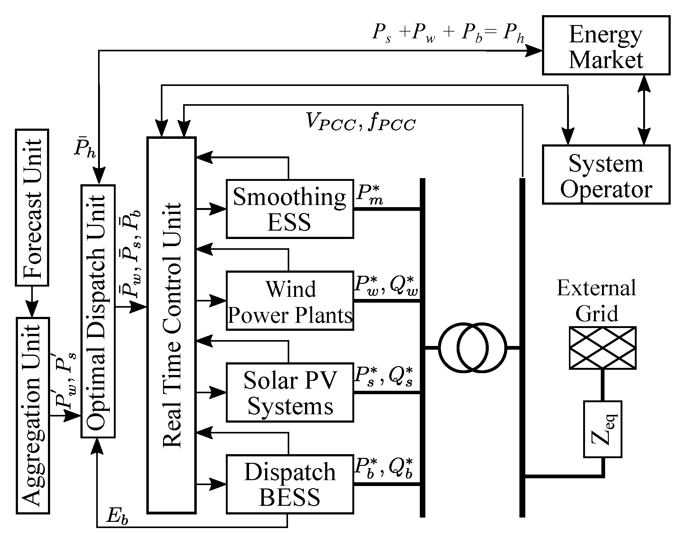
2. Dispatchable Hybrid Power Plant Framework

An energy management system is a key component for realizing dispatchable power from a hybrid renewable power plant. Its role is to continuously assess the available resources to identify the dispatchable power and control the resources to realize the committed power. Therefore, 4 main units are expected for such an energy management system, forecasting (to forecast wind speed, solar irradiance, temperature, etc), aggregation (to estimate the available renewable power at every moment), optimal dispatch, and real-time control, as seen in Figure 1. The focus of this paper is on the optimal dispatch unit. This unit finds the optimum set-points for the wind farm, solar photovoltaic (PV) system, and BESS based on the estimated available renewable power and the state of charge of BESS such that the equipment (and grid code) constraints are respected. These values shall be used for participation of the DHRB in the ICM. It is worth mentioning that in this framework, the output of the forecast and aggregation units [31] is the forecast power corresponding to the lower confidence limit at a sufficiently high confidence level.

3. Hybrid Power Plant Dispatch

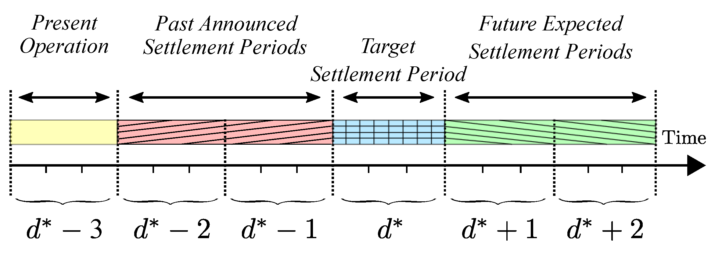
3.1. Dispatch Time Horizons

GENCOs participating in the ICM are required to submit the volume of electricity that they can provide as well as the least acceptable price (market order) $n_D^{-}$ settlement periods ahead (e.g., 2 settlement periods in Ireland [32]) of the target settlement period $d^{*}$. To meet technical constraints and grid code requirements, GENCOs may also consider $n_D^{+}$ post-target settlement periods in their resource assessment. Therefore, at every moment, from a GENCO’s perspective, the ahead settlement periods (as shown in Figure 2), where $n_D^{+}=n_D^{-}=2$, shall be divided into 4 types:

• present operation ($d^{*}-n_D^{-}-1$), which corresponds to the real-time operation of the DHRB, based on the committed power, and is dealt with by the real-time control unit (Figure 1).
• past announced ($d^{*}-n_D^{-}$ to $d^{*}-1$), for which the DHRB operator has already bid in the electricity market and should realize the committed power despite the changes that might have occurred in the available renewable generation forecast to avoid power shortage penalty.
• target ($d^{*}$), which is the nearest (in time) settlement period for which the DHRB operator shall bid.
• future expected ($d^{*}+1$ to $d^{*}+n_D^{-}$), which provides an indication of the future renewable generation forecast for efficient resource management.

3.2. Optimal Scheduling Problem

Considering the former 3 types of settlement periods, an optimization problem is formulated to find the optimal dispatchable power from DHRB. This can be used by GENCO to participate in the ICM. The constraints and objective function are explained in detail.

3.2.1. Constraints

$${\displaystyle P_{h,d}=\sum _{s=1}^S{P}_{s,t_d}+\sum _{w=1}^W{P}_{w,t_d}+\sum _{b=1}^B{P}_{b,t_d}\forall t_d\in T_d}$$

(1)

$${\displaystyle P_{w,t_d}={\lambda }_{w,t_d}{P}_{w,t_d}^{\prime }}$$

(2)

$${\displaystyle P_{s,t_d}={\lambda }_{s,t_d}{P}_{s,t_d}^{\prime }}$$

(3)

$${\displaystyle P_{b,t_d}=P_{b,dc,t_d}{\delta }_{b,dc}-P_{b,c,t_d}{\delta }_{b,c}^{-1}}$$

(4)

$${\displaystyle E_{b,t_d}{N}_D{N}_T=(N_D{N}_T-{\delta }_{b,e})E_{b,t_{d-1}}+P_{b,c,t_d}-P_{b,dc,t_d}}$$

(5)

$$d<d^{*}⟶P_{h,d}={\overline{P}}_{h,d},$$

(6)

where $P_{b,dc,t_d}={\lambda }_{b,dc,t_d}{P}_{b,dc,t_d}^{max}$ and $P_{b,c,t_d}={\lambda }_{b,c,t_d}{P}_{b,c,t_d}^{max}$. S ($s\in S$), W ($w\in W$), B ($b\in B$), D ($d\in D$), and $T_d$ ($t_d\in T_d$) are sets of solar PV system, wind farm, BESS, dispatch interval, and time steps within d, respectively. The DHRB active power and its announced value to the market operator are $P_h$ and ${\overline{P}}_h$, respectively. $P_w$, $P_s$, ${\lambda }_w$, ${\lambda }_s$, $P_w^{\prime }$, and $P_s^{{}^{\prime }}$ are the wind farm and solar PV systems active power set-point, utilization factor of the available power, and forecast power, respectively. $E_b$, ${\delta }_{b,e}$$P_b$, $P_{b,c}$, $P_{b,dc}$, $P_{b,c}^{max}$, $P_{b,dc}^{max}$, ${\lambda }_{b,c}$, ${\lambda }_{b,dc}$, ${\delta }_{b,c}$, and ${\delta }_{b,dc}$ are the BESS stored energy, hourly self-discharge percentage, active power set-point, charge and discharge power, maximum rate, utilization factor, and efficiency, respectively.

Equation (1) requires the power output of the hybrid power plant to be constant during every settlement period d by adjusting the set-points of the wind farm, solar PV system, and BESS for the time steps within d. The active power output of the wind farm, solar PV system, and BESS are defined by (2)–(4), respectively. The stored energy in the BESS at the end of every time step is dependent on the state of charge at the end of the previous time step as well as the power injected/drawn by the BESS in the current time step; this is given by (5). Equation (6) requires the output of the hybrid power plant during the past announced settlement periods to be equal to the submitted values to the system operator. Further constraints can be found in Appendix A.

3.2.2. Objective Function

$${\displaystyle \mathrm{Max}\left\{\sum _{d=d^{*}-n_D^{-}}^{d^{*}+n_D^{+}}\frac{P_{h,d}}{N_D}(C_{h,d}+C_{h,d}^{add})-\sum _{d=d^{*}-n_D^{-}}^{d^{*}+n_D^{+}}\sum _{t_d\in T_d}\sum _{b=1}^B\frac{C_b{\chi }_{b,t_d}}{{\chi }_{b,total}}{(1+{\mathsf{\Pi }}_b)}^{\frac{N_{h,i,d}}{f_{h,\rho }}}\right\},}$$

(7)

where

$$C_{h,d}=\min (C_{h,d}^{\prime }+C_h^{prem},C_h^{cap})$$

$$N_{h,i,d}=⌊\frac{8760}{N_{\rho }}\mathit{frac}\left(\frac{d-1}{8760N_D}\right)⌋+1+n_{\rho }+⌊\frac{d-1}{8760N_D}⌋f_{h,\rho },$$

$${\chi }_{b,t_d}=\frac{E_{b,t_d-1}{\delta }_{b,e}+{\lambda }_{b,c,t_d}{P}_{b,c}^{max}+{\lambda }_{b,dc,t_d}{P}_{b,dc}^{max}}{N_D{N}_T}$$

$${\chi }_{b,total}=({\lambda }_{b,e}^{max}-{\lambda }_{b,e}^{min}){\delta }_{b,c}{\delta }_{b,dc}{E}_b^{max}(N_b+1)(EO{L}_b+1)$$

and $C_{h,d}^{\prime }$, $C_h^{prem}$, $C_h^{add}$, $C_h^{cap}$, $EO{L}_b$, $N_b$, $N_{\rho }$, and $n_{\rho }$ are the expected ICM clearing price, premium paid to support renewable, any other additional income or penalty per injected energy (e.g., balancing cost) and cap for payment to renewable [33], BESS end-of-life per-unit capacity, nominal BESS charge cycles, number of hours covered per payment, and number of intervals for delay in payment, respectively. The second term in Equation (7) approximates the cost associated with the degradation of BESS considering the yearly interest rate ${\mathsf{\Pi }}_b$ for BESS capital cost $C_b$ and frequency of payment per year for DHRB $f_{h,\rho }$.

3.2.3. Problem Definition

The revenue maximization (RM) problem is defined based on the presented constraints and objective function:

• Constraints: (1)–(6) and (A1)–(A8);
• Objective function: (7);
• Decision variables: $P_{b,c}$, $P_{b,dc}$, $P_s$, and $P_w$.

3.3. Robust Optimal Scheduling Problem

The presented RM optimization problem assumes that the expected ICM price will be realized; however, this value is uncertain due to its dependence on the matching market order. To take this aspect into account, the methodology presented by [34] is employed. With this methodology, the actual purchase price of electricity is

$$C_{h,d}+\mathsf{\Delta }{C}_{h,d}^{+}{\mathsf{\Lambda }}_{h,d}^{+}+\mathsf{\Delta }{C}_{h,d}^{-}{\mathsf{\Lambda }}_{h,d}^{-},$$

where $\mathsf{\Delta }{C}_{h,d}^{+}$ and $\mathsf{\Delta }{C}_{h,d}^{-}$ are the maximum and minimum power purchase price change, respectively; these are defined as

$$\mathsf{\Delta }{C}_{h,d}^{+}=\min (C_{h,d}^{+}+C_h^{prem},C_h^{cap})-C_{h,d}$$

$$\mathsf{\Delta }{C}_{h,d}^{-}=\min (C_{h,d}^{-}+C_h^{prem},C_h^{cap})-C_{h,d}$$

The application factors ${\mathsf{\Lambda }}_{h,d}^{+}$ and ${\mathsf{\Lambda }}_{h,d}^{-}$ are defined over the $\left[01\right]$ interval. In any electricity price scenario, $O_{{\mathsf{\Phi }}_h}^k$ (where $k\in K$ and K is the set of price scenarios), the condition ${\mathsf{\Lambda }}_{h,d}^{+}\ast {\mathsf{\Lambda }}_{h,d}^{-}=0$ and ${\displaystyle \sum _{d=d^{*}-n_D^{-}}^{d^{*}+n_D^{+}}{\mathsf{\Lambda }}_{h,d}^{-}\le {\mathsf{\Phi }}_h}$ must hold. The use of BESS may become inefficient if the ICM price is lower than predicted, i.e., ${\mathsf{\Lambda }}_{h,d}^{-}>0$. For fixed $P_{b,c}$, $P_{b,dc}$, $P_s$, and $P_w$, the worst electricity price scenario $O_{{\mathsf{\Phi }}_h}^{worst}$ is the scenario at which ${\mathsf{\Lambda }}_{h,d}^{-}=1$ in up to ${\mathsf{\Phi }}_h$ dispatch intervals. Hence, $O_{{\mathsf{\Phi }}_h}^{worst}$ can be found by solving

$$\begin{array}{cc}\hfill & {\displaystyle \mathrm{Min}\sum _{d=d^{*}-n_D^{-}}^{d^{*}+n_D^{+}}\frac{P_{h,d}}{N_D}\mathsf{\Delta }{C}_{h,d}^{-}{\mathsf{\Lambda }}_{h,d}^{-}}\hfill \\ s.t.\hfill & {\displaystyle \sum _{d=d^{*}-n_D^{-}}^{d^{*}+n_D^{+}}{\mathsf{\Lambda }}_{h,d}^{-}\le {\mathsf{\Phi }}_h}\hfill \\ \hfill & 0\le {\mathsf{\Lambda }}_{h,d}^{-}\le 1,\hfill \end{array}$$

(8)

where the parameter ${\mathsf{\Phi }}_h$ is referred to as the uncertainty budget. Accordingly, in any $O_{{\mathsf{\Phi }}_h}^k$ other than $O_{{\mathsf{\Phi }}_h}^{worst}$, the fixed variables will lead to a greater or equal DHRB income.

It can be noted that $P_{h,d}$ affect $O_{{\mathsf{\Phi }}_h}^{worst}$. However, robust operation of the DHRB entails optimizing against the worst-case scenario (maximizing the minimum income, i.e., Maximin). This implies that a mixed-integer nonlinear programming (MINLP) problem (combining (8) and RM) needs to be solved. Bilevel optimization techniques can be employed to handle this problem by solving RM and (8) iteratively. However, iterative approaches may not be ideal due to convergence issues. Therefore, the bilevel problem is converted to a unilevel MILP problem using the duality theory. Accordingly, a new objective function and constraint are defined by (9) and (10), respectively.

$$\begin{array}{cc}{\displaystyle \mathrm{Max}}\hfill & {\displaystyle \left\{\sum _{d=d^{*}-n_D^{-}}^{d^{*}+n_D^{+}}\frac{P_{h,d}}{N_D}(C_{h,d}+C_{h,d}^{add})-\sum _{d=d^{*}-n_D^{-}}^{d^{*}+n_D^{+}}\sum _{t_d\in T_d}\sum _{b=1}^B\frac{C_b{\chi }_{b,t_d}}{{\chi }_{b,total}}{(1+{\mathsf{\Pi }}_b)}^{\frac{N_{h,i,d}}{f_{h,\rho }}}\right.}\hfill \\ \hfill \\ \hfill & {\displaystyle -\left.\sum _{d=d^{*}-n_D^{-}}^{d^{*}+n_D^{+}}{\mathsf{\Psi }}_{h,d}-{\xi }_h{\mathsf{\Phi }}_h\right\}}\hfill \\ \hfill \end{array}$$

(9)

$$-{\mathsf{\Psi }}_{h,d}-{\xi }_h\le \frac{P_{h,d}}{N_D}\mathsf{\Delta }{C}_{h,d}^{-},$$

(10)

where ${\mathsf{\Psi }}_{h,d}$ and ${\xi }_h$ are non-negative dual variables yielded from (8). Subsequently, the robust revenue maximization (RRM) problem is given:

• Constraints: (1)–(6), (10) and (A1)–(A8);
• Objective function: (9);
• Decision variables: ${\mathsf{\Psi }}_{h,d}$, ${\xi }_h$, $P_{b,c}$, $P_{b,dc}$, $P_s$ and $P_w$.

This problem finds DHRB set-points $S{P}_{{\mathsf{\Phi }}_h}$ that maximize the minimum income if ${\displaystyle \sum _{d=d^{*}-n_D^{-}}^{d^{*}+n_D^{+}}{\mathsf{\Lambda }}_{h,d}^{-}\le {\mathsf{\Phi }}_h}$. Hence, $S{P}_0$ is identical to the set-points found in the RM problem. Further details on the applied technique can be found in [34].

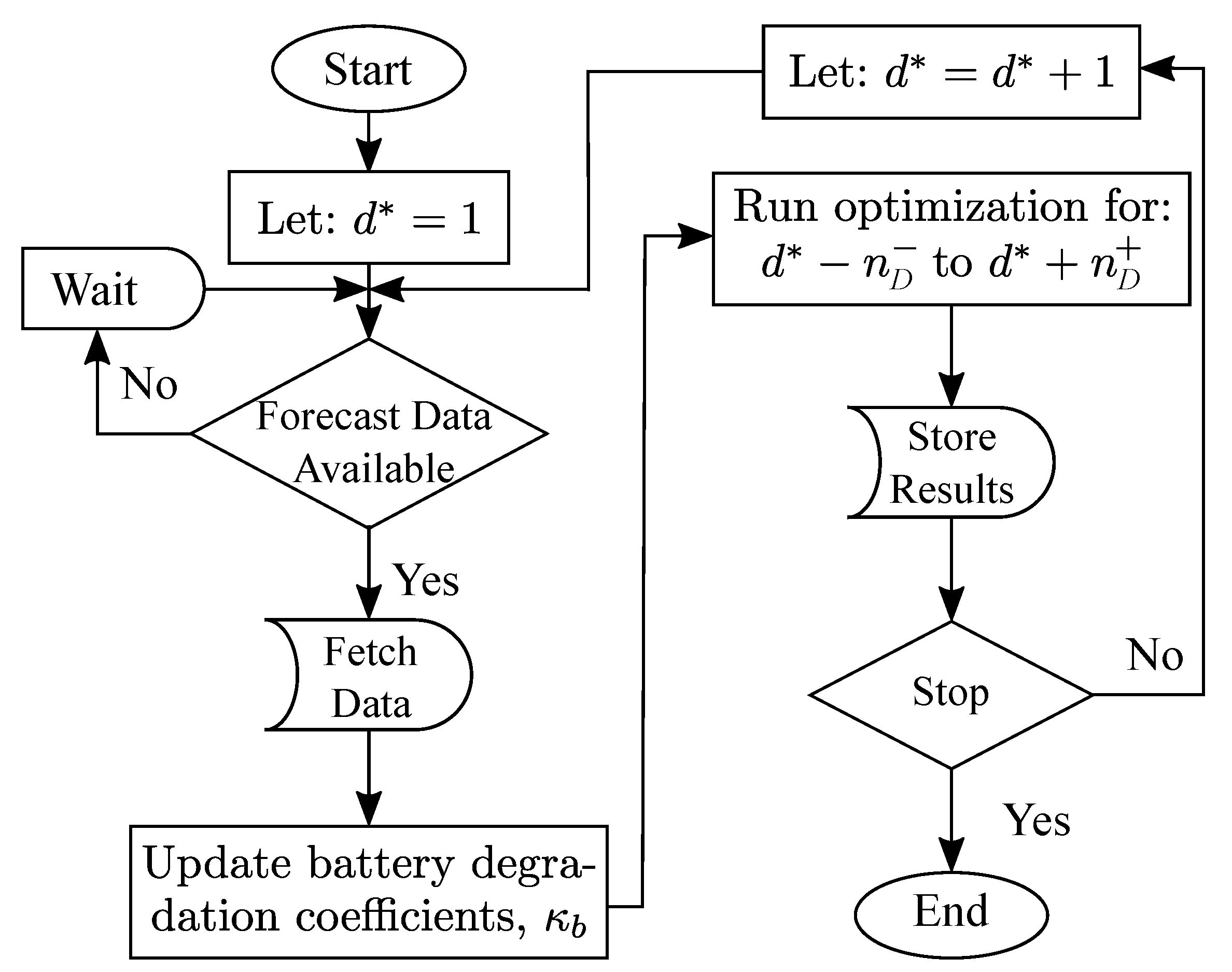
3.4. Rolling Approach

The rolling algorithm shown by Figure 3 is used to solve the RRM problem for the $d^{*}-n_D^{-}$ to $d^{*}+n_D^{+}$ settlement periods window and identify the dispatchable power for the target settlement period and meet the committed power in the past announced settlement periods. In every iteration, this algorithm updates the forecast and battery degradation coefficients (per Appendix B) for $d^{*}-n_D^{-}$ to $d^{*}+n_D^{+}$ to improve accuracy. This gives the DHRB operator the ability to adjust the forecast and aggregation units’ parameters where necessary.

As implied, the proposed framework is capable of handling multiple resources and associated forecasts. However, for it to efficiently deliver dispatchable renewable generation, it is necessary to adequately size the BESS both in terms of capacity and rate of charge and discharge. Sizing the resources is out of the scope of this paper; however, more details can be found in [9,35,36].

4. Case Study

A case study was carried out on an 80-MW hybrid renewable power plant comprising a 50 MW wind farm, 30 MW solar PV system, and 5 MWh BESS. The length of each settlement period was assumed to be 30 min ($N_D=2$). One-year, 10-min resolution ($N_T=3$) wind and solar power generation profiles obtained from [37] were used as input (assumed as output of the aggregation unit in Figure 1). Ten years of electricity market data obtained from [32] was used to form the 1 year maximum and minimum ICM price profiles ($C_h^{+}$ and $C_h^{-}$) and expected ICM price profile ($C_h^{\prime }$); however, these could be produced with certain confidence levels using forecasting techniques (e.g., ARIMA [29]). Short-term balancing cost increase due to the intermittency of renewables is assumed €3/MWh; since a DHRB guarantees the dispatch, the short-term balancing cost can be avoided and deemed as a potential income for the DHRB, i.e., $C_h^{add}=$ €3/MWh. The parameters are summarized in

Table 1. List of parameters.

Parameter	Value	Parameter	Value	Parameter	Value
$E_b^{max}$	5 MWh	${\lambda }_{b,e}^{max}$	1	${\lambda }_{b,e}^{min}$	0.2
$P_{b,c}^{max}$	10 MW	${\lambda }_{b,c}^{max}$	1	${\lambda }_{b,c}^{min}$	0
$P_{b,dc}^{max}$	10 MW	${\lambda }_{b,dc}^{max}$	1	${\lambda }_{b,dc}^{min}$	0
$P_w^{max}$	50 MW	${\lambda }_w^{max}$	1	${\lambda }_w^{min}$	0
$P_w^{min}$	30 MW	${\lambda }_s^{max}$	1	${\lambda }_s^{min}$	0
$EO{L}_b$	0.65	$N_{\rho }$	730	${\delta }_{b,e}$	0.005%
$C_h^{prem}$	30$\frac{\mathsf{€}}{\mathrm{MWh}}$	$f_{h,\rho }$	12	${\delta }_{b,c}$	0.95
$C_h^{cap}$	77$\frac{\mathsf{€}}{\mathrm{MWh}}$	$n_{\rho }$	0	${\delta }_{b,dc}$	0.95
$C_b$	€1.5m	${\mathsf{\Pi }}_b$	0.04	$N_b$	4000

.

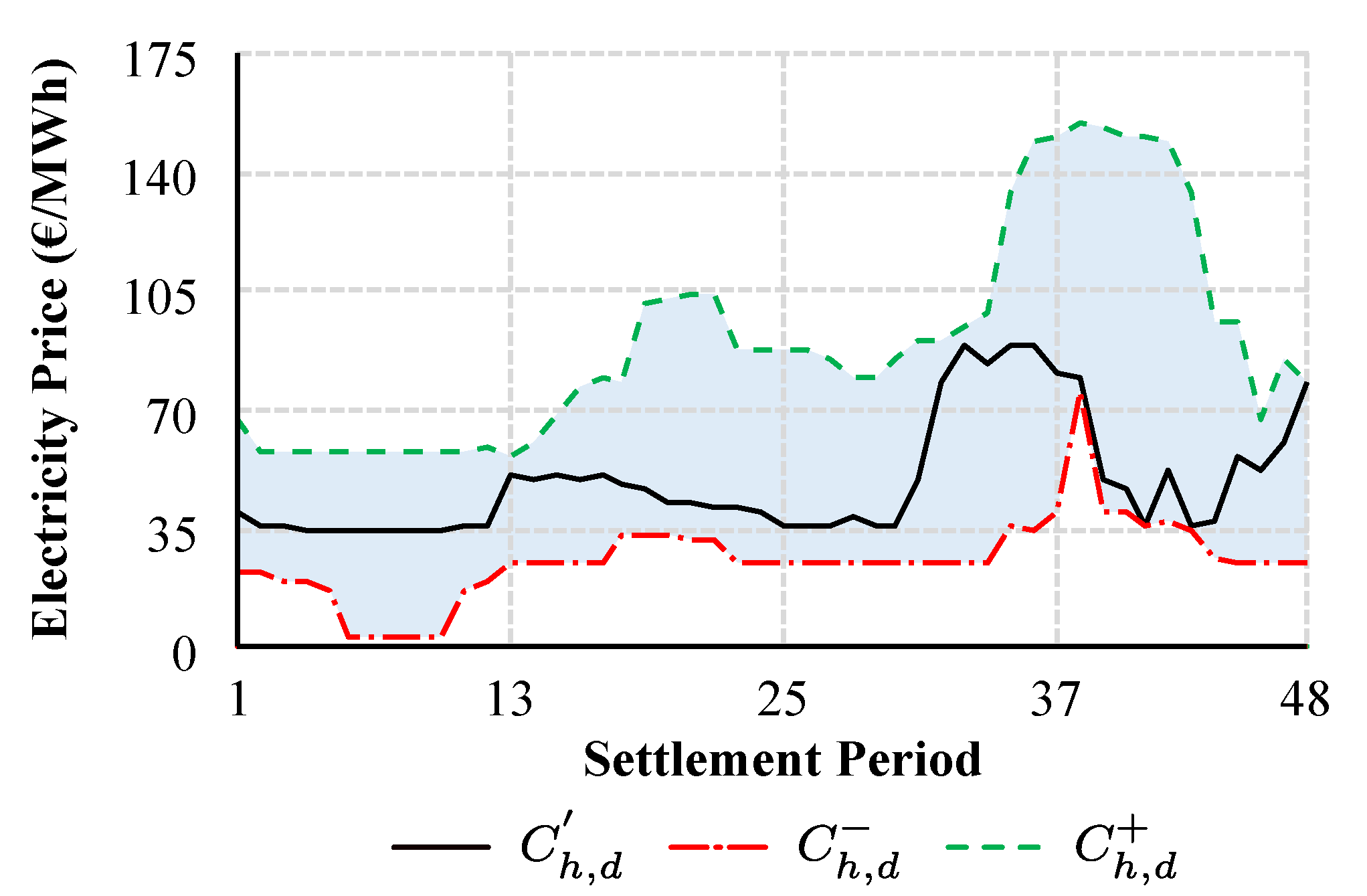
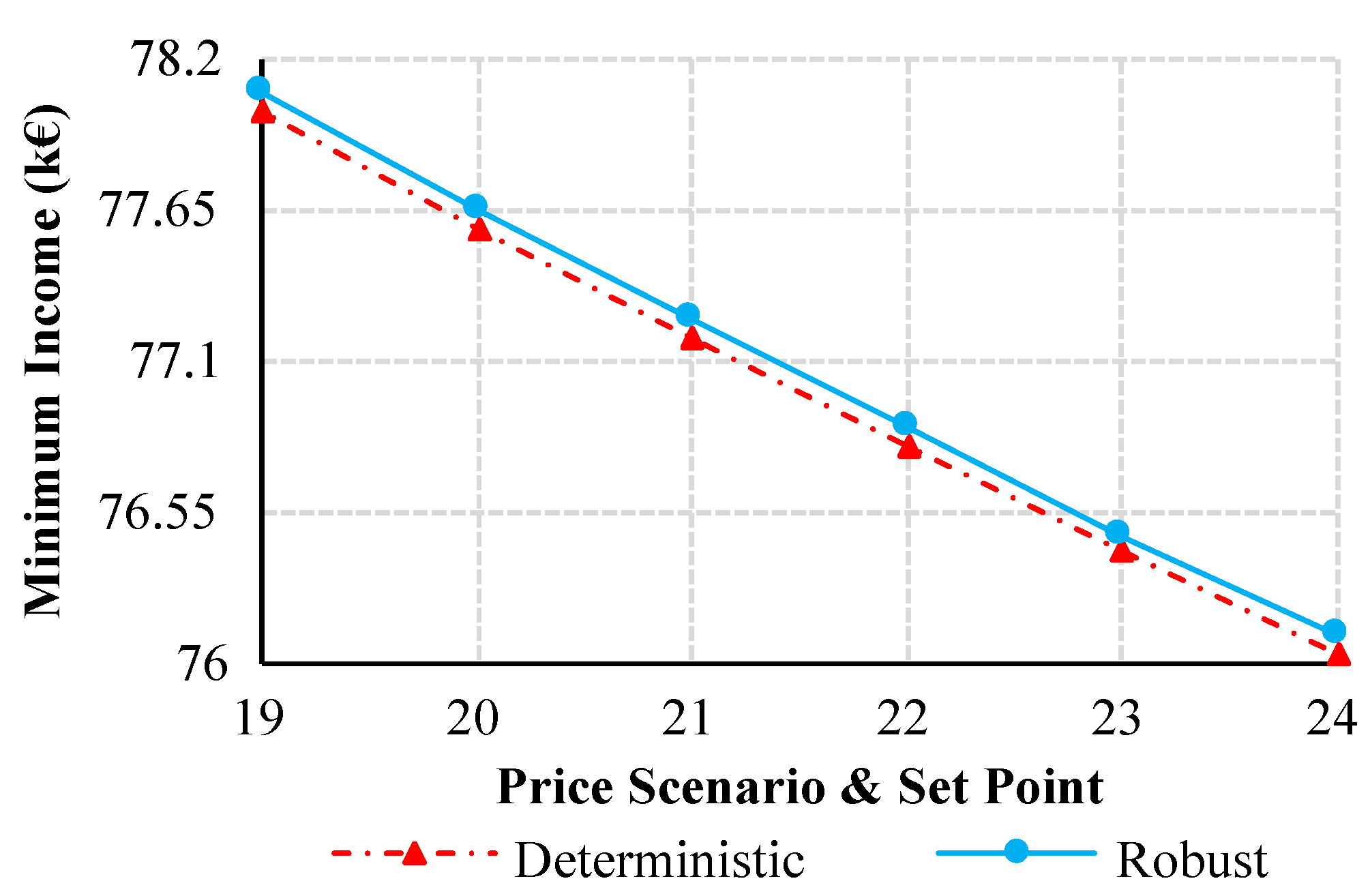
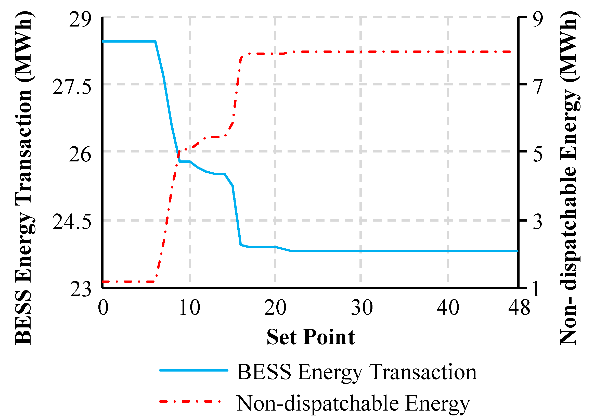
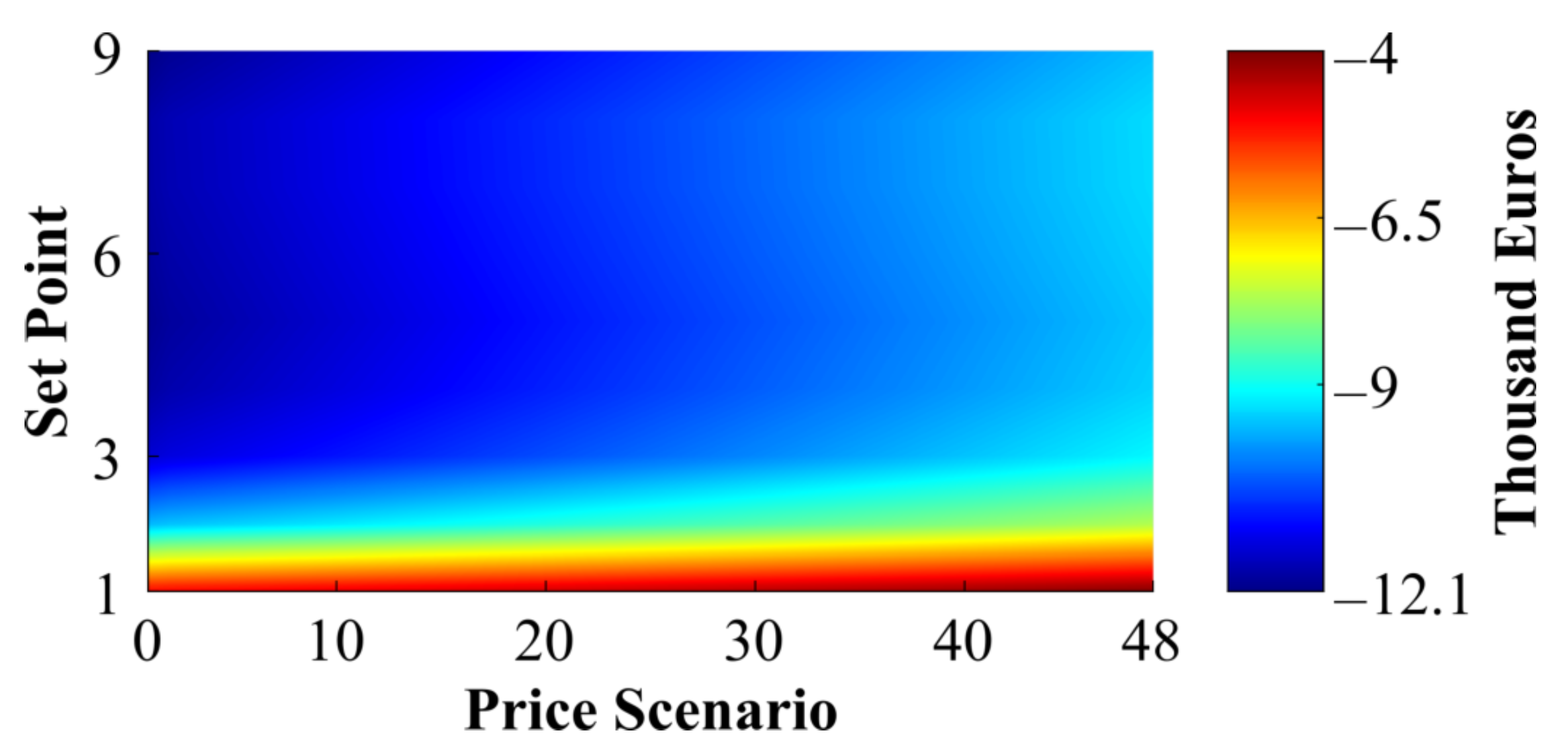
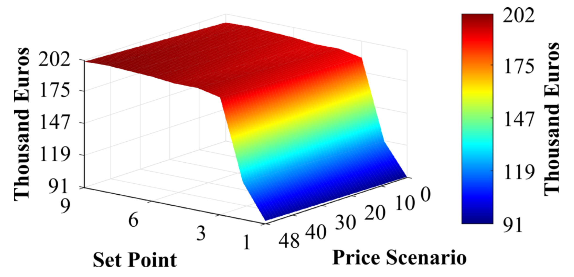
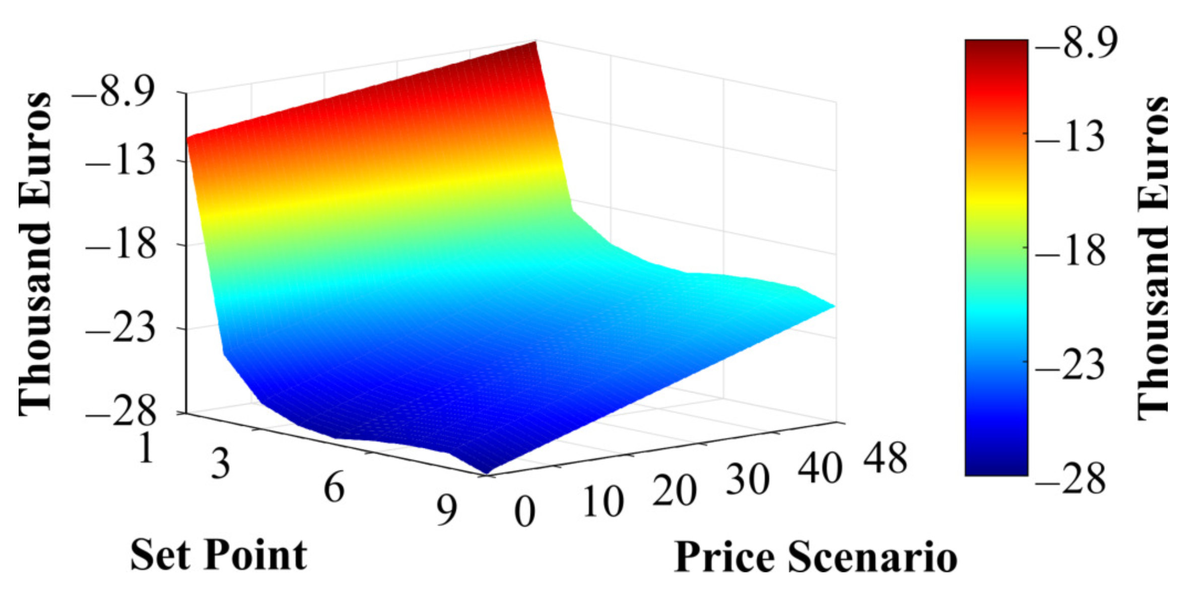
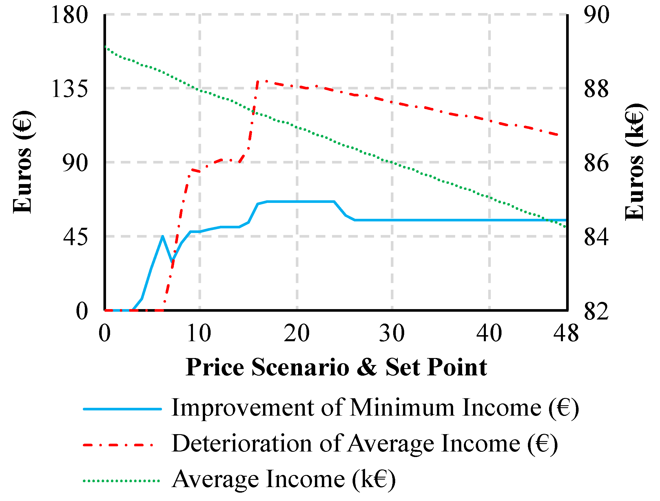
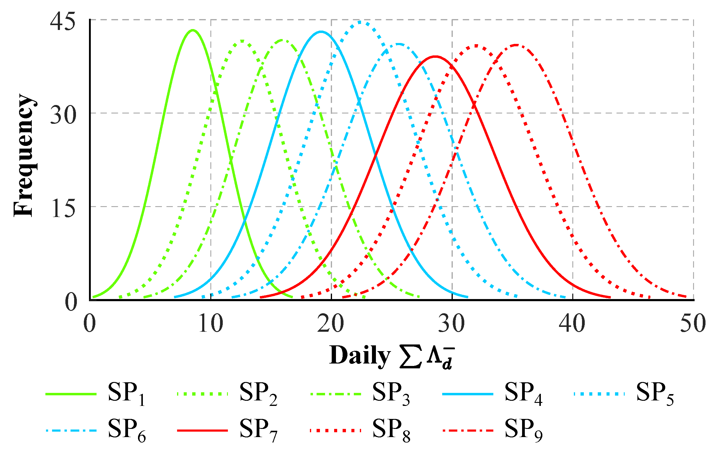
4.1. Effect of Uncertainty Degree

Figure 4 shows $C^{\prime }$, $C^{+}$, and $C^{-}$ ICM price profiles for 1 day, with 48 settlement periods. It can be seen that while the difference between the expected and the minimum electricity price is negligible in some of the settlement periods, in others it reaches up to 82%. The realization of the lower electricity prices may contradict the economic justification of using BESS to realize dispatchable renewable generation.

Initially, the effect of the uncertainty degree was investigated. In the day of interest, $S{P}_{{\mathsf{\Phi }}_h}$ were found for ${\mathsf{\Phi }}_h$ ranging from 1 to 48. For this purpose, the RRM problem was solved in single runs, i.e., without the rolling algorithm ($n_D^{-}=1$ and $n_D^{-}=47$). $S{P}_{{\mathsf{\Phi }}_h}$ were then used to calculate the income of the DHRB in the corresponding $O_{{\mathsf{\Phi }}_h}^{worst}$. In Figure 5, this is compared to the minimum income of the DHRB, at various ${\mathsf{\Phi }}_h$, if $S{P}_0$ is used instead.

It can be seen that for every ${\mathsf{\Phi }}_h$ shown, using $S{P}_{{\mathsf{\Phi }}_h}$ results in a greater (or equal) worst DHRB income compared with using $S{P}_0$. However, by using $S{P}_{{\mathsf{\Phi }}_h}$, there is a risk of loss of income if price scenarios other than $O_{{\mathsf{\Phi }}_h}^{worst}$ are realized. This is shown with the aid of ≈2 million random-generated $O_{{\mathsf{\Phi }}_h}^k$ (within $C_{h,d}^{-}$ and $C_{h,d}^{+}$). The average DHRB income using $S{P}_{{\mathsf{\Phi }}_h}$ in $O_{{\mathsf{\Phi }}_h}^k$ was calculated. This was then compared with the average DHRB income using $S{P}_0$ in the same $O_{{\mathsf{\Phi }}_h}^k$ to yield the average income deterioration trend. The trends for improvement of minimum income and deterioration of average income are shown in Figure 6. It can be seen that at certain $\mathsf{\Phi }$, the risk of using $S{P}_{{\mathsf{\Phi }}_h}$ instead of $S{P}_0$ is higher than its benefit. It should be noted that the drops and rises in the improvement and deterioration trends are due to the change in the difference between the DHRB income in the corresponding price scenarios and should not be mistaken with the actual DHRB income.

As illustrated in Figure 7, by using $S{P}_{{\mathsf{\Phi }}_h}$, the BESS energy transaction reduced when $\mathsf{\Phi }$ increased. The effect of less usage of BESS manifested in the nondispatchable energy, which followed a similar but inverse trend. Interestingly, this is in the favor of DHRB minimum income (per Figure 5). It means that compared to using $S{P}_{{\mathsf{\Phi }}_h}$, $S{P}_0$ not only leads to lower minimum income but also further exhausts BESS.

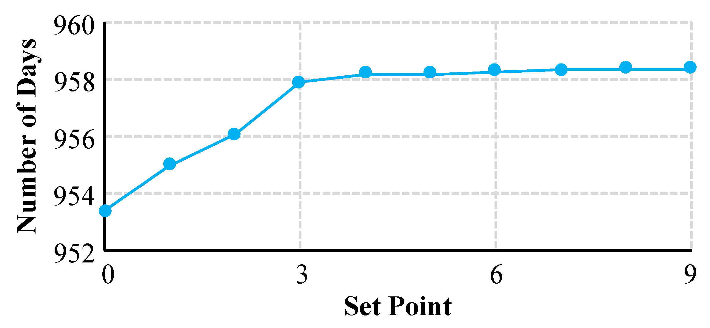
4.2. Invoking the Rolling Algorithm

The characteristics of the RRM problem when used within a rolling algorithm were investigated by solving it for 1-year operation of the DHRB using a sliding window of 10 settlement periods ($n_D^{-}=2$ and $n_D^{-}=6$) for uncertainty degrees ranging from 1 to 9. The rolling algorithm updates $S{P}_{{\mathsf{\Phi }}_h}$ and, consequently, $O_{{\mathsf{\Phi }}_h}^{worst}$ in every run; therefore, ${\mathsf{\Lambda }}_d^{-}$ is only fixed when d leaves the sliding window. This means that $\sum {\mathsf{\Lambda }}_d^{-}<=\mathsf{\Phi }$ may not hold for every 10 consecutive settlement periods or even be consistent over the days. Figure 8 shows the 1-year normal distribution fit of daily $\sum {\mathsf{\Lambda }}_d^{-}$ that resulted in $S{P}_{{\mathsf{\Phi }}_h}$. Despite the inconsistency, it can be seen that the mean value of $\sum {\mathsf{\Lambda }}_d^{-}$ increased with ${\mathsf{\Phi }}_h$.

For the day of interest of Section 4.1, Figure 9 shows the average change of DHRB income (over the same random $O_{{\mathsf{\Phi }}_h}^k$) if $S{P}_{{\mathsf{\Phi }}_h}$ is used instead of $S{P}_0$. Interestingly, the income improved slightly with $S{P}_1$; however, for the rest of the $S{P}_{{\mathsf{\Phi }}_h}$, the DHRB income deteriorated. The maximum deterioration occurred at $S{P}_6$, which is worst than the maximum deterioration seen in Figure 6, where a rolling algorithm was not invoked (e.g., day ahead market).

To explore the applicability of the RRM as a year-long solution (with rolling algorithm), ≈2 million year-long random $O_{{\mathsf{\Phi }}_h}^k$ (within $C_{h,d}^{-}$ and $C_{h,d}^{+}$) with ${\mathsf{\Phi }}_h$ ranging from 1 to 48 (within a day) were generated. The average change of 1-year DHRB income if $S{P}_{{\mathsf{\Phi }}_h}$ is used instead of $S{P}_0$ is shown in Figure 10. It can be seen that for all of $S{P}_{{\mathsf{\Phi }}_h}$, the average change of income is negatively indicating that it deteriorated. The reason behind this phenomenon is the nondispatchable energy. Figure 11 shows the total DHRB nondispatchable energy and BESS energy transaction in 1-year operation with each of the studied $S{P}_{{\mathsf{\Phi }}_h}$.

It is inferred that less use of BESS in vulnerable settlement periods increased the total power plant nondispatchable energy, hence the reduced income of DHRB. It should be noted that the change in the total DHRB nondispatchable energy and BESS energy transaction may not necessarily be equal since this change might correspond to only fractions of the settlement period that are not equal in length.

To capture the benefit of the difference noted in the BESS energy transaction, the simulation was extended to the end of the life of BESS by duplicating the 1-year renewables and electricity price profiles. For each $S{P}_{{\mathsf{\Phi }}_h}$, Figure 12 shows the number of days the BESS could be operated before its end of life. It can be seen that up to $S{P}_3$, the lifetime of BESS increased linearly, however, it saturated after that. This is in line with the total BESS energy transaction trend shown in Figure 11.

Two situations were considered:

• Situation A: DHRB stopping power injection after BESS lifetime;
• Situation B: DHRB committed to injecting the minimum predicted renewable power (within each d), until the d corresponding to BESS’ end of life with $S{P}_9$ is completed, i.e., d = 46,003.

The latter is a hypothetical situation, which was solely considered for comparison purpose. The change in lifetime average DHRB income (over the random $O_{{\mathsf{\Phi }}_h}^k$) if $S{P}_{{\mathsf{\Phi }}_h}$ is used instead of $S{P}_0$ has been calculated for situations A and B and is shown in Figure 13 and Figure 14, respectively.

It can be seen that in situation A, compared to $S{P}_0$, the average extra income of DHRB through the BESS lifetime is ≈€$91k$ when $S{P}_1$ is used. This number can reach up to ≈€$202k$ by using $S{P}_9$. A slight increase is also noted comparing $O_{48}^k$ with $O_1^k$. This means that the more the number of hours, the more the electricity price differs from the expected value, and the more the average extra income will be if $S{P}_{{\mathsf{\Phi }}_h}$ is used instead of $S{P}_0$. However, the change of the income in situation B exhibited a different behavior, which is similar to that illustrated in Figure 10. It can be noted that using $S{P}_{{\mathsf{\Phi }}_h}$ instead of $S{P}_0$ results in a reduction of the average lifetime DHRB income. This reduction is largest for $S{P}_3$ onward. Although, the loss of income reduces as the number of hours the electricity price differs from the expected value increases.

5. Conclusions

This paper explored the participation of a dispatchable hybrid renewable solar–wind power plant with a battery energy storage system in the intraday continuous electricity market. Economic justification of BESS operation in a DHRB can be jeopardized by the uncertain electricity price. Duality theory was employed to derive a unilevel MILP problem for robust optimization of DHRB set-points. Implications of using robust optimization for short-term and long-term operation of DHRB and BESS lifetime were investigated. With the aid of a sensitivity analysis, it was shown that robust optimization improves the minimum income of DHRB; however, it may not yield the optimum solution if the electricity price differs from the worst scenario. Hence, there will be a risk of loss of income for DHRB. The loss of income is associated with the increased DHRB nondispatchable energy. However, this phenomenon was accompanied by slightly reduced BESS energy transaction, which in turn resulted in its longer lifetime. Therefore, over the lifetime of BESS, on average (over a large set of electricity price scenarios), the income of DHRB was higher comparing robust to deterministic optimization. The methodology presented can help to optimize the planning and operation of DHRB.

References

1. Ye, H.; Wang, J.; Ge, Y.; Li, J.; Li, Z. Robust Integration of High-Level Dispatchable Renewables in Power System Operation. IEEE Trans. Sustain. Energy 2017, 8, 826–835. [Google Scholar] [CrossRef]
2. Blakers, A.; Stocks, M.; Lu, B.; Cheng, C.; Stocks, R. Pathway to 100% Renewable Electricity. IEEE J. Photovolt. 2019, 9, 1828–1833. [Google Scholar] [CrossRef]
3. Bakhtvar, M.; Al-Hinai, A.; Moursi, M.S.E.; Albadi, M.; Al-Badi, A.; Maashri, A.A.; Abri, R.A.; Hosseinzadeh, N.; Charaabi, Y.; Al-Yahyai, S. Optimal Scheduling for Dispatchable Renewable Energy Generation. In Proceedings of the 2020 6th IEEE International Energy Conference (ENERGYCon), Tunis, Tunisia, 28 September–1 October 2020; pp. 238–243. [Google Scholar]
4. Nguyen, C.; Lee, H. Effective power dispatch capability decision method for a wind-battery hybrid power system. IET Gener. Transm. Distrib. 2016, 10, 661–668. [Google Scholar] [CrossRef]
5. Abdullah, M.A.; Muttaqi, K.M.; Sutanto, D.; Agalgaonkar, A.P. An Effective Power Dispatch Control Strategy to Improve Generation Schedulability and Supply Reliability of a Wind Farm Using a Battery Energy Storage System. IEEE Trans. Sustain. Energy 2015, 6, 1093–1102. [Google Scholar] [CrossRef]
6. Gholami, M.; Fathi, S.H.; Milimonfared, J.; Chen, Z.; Deng, F. A new strategy based on hybrid battery–wind power system for wind power dispatching. IET Gener. Transm. Distrib. 2018, 12, 160–169. [Google Scholar] [CrossRef]
7. Zhang, F.; Hu, Z.; Meng, K.; Ding, L.; Dong, Z.Y. Sequence control strategy for hybrid energy storage system for wind smoothing. IET Gener. Transm. Distrib. 2019, 13, 4482–4490. [Google Scholar] [CrossRef]
8. Wee, K.W.; Choi, S.S.; Vilathgamuwa, D.M. Design of a Least-Cost Battery-Supercapacitor Energy Storage System for Realizing Dispatchable Wind Power. IEEE Trans. Sustain. Energy 2013, 4, 786–796. [Google Scholar] [CrossRef]
9. Bakhtvar, M.; Al-Hinai, A.; El Moursi, M.S.; Albadi, M. A Vision of Flexible Dispatchable Hybrid Solar-Wind-Energy Storage Power Plant. IET Renew. Power Gener. 2021, 15, 1848–1860. [Google Scholar]
10. Teleke, S.; Baran, M.E.; Bhattacharya, S.; Huang, A.Q. Rule-Based Control of Battery Energy Storage for Dispatching Intermittent Renewable Sources. IEEE Trans. Sustain. Energy 2010, 1, 117–124. [Google Scholar] [CrossRef]
11. Li, X.; Hui, D.; Lai, X. Battery Energy Storage Station (BESS)-Based Smoothing Control of Photovoltaic (PV) and Wind Power Generation Fluctuations. IEEE Trans. Sustain. Energy 2013, 4, 464–473. [Google Scholar] [CrossRef]
12. Lilla, S.; Orozco, C.; Borghetti, A.; Napolitano, F.; Tossani, F. Day-Ahead Scheduling of a Local Energy Community: An Alternating Direction Method of Multipliers Approach. IEEE Trans. Power Syst. 2020, 35, 1132–1142. [Google Scholar] [CrossRef]
13. Pal, P.; Krishnamoorthy, P.A.; Rukmani, D.K.; Antony, S.J.; Ocheme, S.; Subramanian, U.; Elavarasan, R.M.; Das, N.; Hasanien, H.M. Optimal Dispatch Strategy of Virtual Power Plant for Day-Ahead Market Framework. Appl. Sci. 2021, 11, 3814. [Google Scholar] [CrossRef]
14. Li, Z.; Shahidehpour, M. Privacy-Preserving Collaborative Operation of Networked Microgrids with the Local Utility Grid Based on Enhanced Benders Decomposition. IEEE Trans. Smart Grid 2020, 11, 2638–2651. [Google Scholar] [CrossRef]
15. Zeinal-Kheiri, S.; Ghassem-Zadeh, S.; Mohammadpour Shotorbani, A.; Mohammadi-Ivatloo, B. Real-time energy management in a microgrid with renewable generation, energy storages, flexible loads and combined heat and power units using Lyapunov optimisation. IET Renew. Power Gener. 2020, 14, 526–538. [Google Scholar] [CrossRef]
16. Neuhoff, K.; Ritter, N.; Salah-Abou-El-Enien, A.; Vassilopoulo, P. Intraday Markets for Power: Discretizing the Continuous Trading? Discussion Paper No. 1544; DIW Berlin: Berlin, Germany, 2016. [Google Scholar]
17. Li, G.; Shi, J.; Qu, X. Modeling methods for GenCo bidding strategy optimization in the liberalized electricity spot market–A state-of-the-art review. Energy 2011, 36, 4686–4700. [Google Scholar] [CrossRef]
18. Bertrand, G.; Papavasiliou, A. Adaptive Trading in Continuous Intraday Electricity Markets for a Storage Unit. IEEE Trans. Power Syst. 2020, 35, 2339–2350. [Google Scholar] [CrossRef]
19. Ansari, B.; Rahimi-Kian, A. A Dynamic Risk-Constrained Bidding Strategy for Generation Companies Based on Linear Supply Function Model. IEEE Syst. J. 2015, 9, 1463–1474. [Google Scholar] [CrossRef]
20. Mohammad, N.; Mishra, Y. Retailer’s risk-aware trading framework with demand response aggregators in short-term electricity markets. IET Gener. Transm. Distrib. 2019, 13, 2611–2618. [Google Scholar] [CrossRef]
21. Vahedipour-Dahraie, M.; Rashidizadeh-Kermani, H.; Anvari-Moghaddam, A. Risk-Based Stochastic Scheduling of Resilient Microgrids Considering Demand Response Programs. IEEE Syst. J. 2021, 15, 971–980. [Google Scholar] [CrossRef]
22. Fleten, S.E.; Kristoffersen, T.K. Stochastic programming for optimizing bidding strategies of a Nordic hydropower producer. Eur. J. Oper. Res. 2007, 181, 916–928. [Google Scholar] [CrossRef] [Green Version]
23. Ospina, J.; Gupta, N.; Newaz, A.; Harper, M.; Faruque, M.O.; Collins, E.G.; Meeker, R.; Lofman, G. Sampling-Based Model Predictive Control of PV-Integrated Energy Storage System Considering Power Generation Forecast and Real-Time Price. IEEE Power Energy Technol. Syst. J. 2019, 6, 195–207. [Google Scholar] [CrossRef]
24. Chang, X.; Xu, Y.; Gu, W.; Sun, H.; Chow, M.Y.; Yi, Z. Accelerated Distributed Hybrid Stochastic/Robust Energy Management of Smart Grids. IEEE Trans. Ind. Inform. 2021, 17, 5335–5347. [Google Scholar] [CrossRef]
25. Daneshvar, M.; Mohammadi-Ivatloo, B.; Zare, K.; Asadi, S. Two-Stage Robust Stochastic Model Scheduling for Transactive Energy Based Renewable Microgrids. IEEE Trans. Ind. Inform. 2020, 16, 6857–6867. [Google Scholar] [CrossRef]
26. Purage, M.I.S.L.; Krishnan, A.; Foo, E.Y.S.; Gooi, H.B. Cooperative Bidding-Based Robust Optimal Energy Management of Multimicrogrids. IEEE Trans. Ind. Inform. 2020, 16, 5757–5768. [Google Scholar] [CrossRef]
27. Li, Y.; Zhao, T.; Liu, C.; Zhao, Y.; Yu, Z.; Li, K.; Wu, L. Day-Ahead Coordinated Scheduling of Hydro and Wind Power Generation System Considering Uncertainties. IEEE Trans. Ind. Appl. 2019, 55, 2368–2377. [Google Scholar] [CrossRef]
28. Liu, Y.; Li, Y.; Gooi, H.B.; Jian, Y.; Xin, H.; Jiang, X.; Pan, J. Distributed Robust Energy Management of a Multimicrogrid System in the Real-Time Energy Market. IEEE Trans. Sustain. Energy 2019, 10, 396–406. [Google Scholar] [CrossRef]
29. Baringo, L.; Conejo, A.J. Offering Strategy Via Robust Optimization. IEEE Trans. Power Syst. 2011, 26, 1418–1425. [Google Scholar] [CrossRef]
30. Wang, L.; Zhu, Z.; Jiang, C.; Li, Z. Bi-Level Robust Optimization for Distribution System With Multiple Microgrids Considering Uncertainty Distribution Locational Marginal Price. IEEE Trans. Smart Grid 2021, 12, 1104–1117. [Google Scholar] [CrossRef]
31. Al-Zadjali, S.; Al Maashri, A.; Al-Hinai, A.; Al-Yahyai, S.; Bakhtvar, M. An Accurate, Light-Weight Wind Speed Predictor for Renewable Energy Management Systems. Energies 2019, 12, 4355. [Google Scholar] [CrossRef] [Green Version]
32. Single Electricity Market Operator. Available online: http://www.sem-o.com (accessed on 13 August 2018).
33. IRENA. 30 Year of Policies for Wind Energy: Lessons from 12 Wind Energy Markets; International Renewable Energy Agency (IRENA): Abu Dhabi, United Arab Emirates, 2016. [Google Scholar]
34. Soroudi, A.; Siano, P.; Keane, A. Optimal DR and ESS Scheduling for Distribution Losses Payments Minimization under Electricity Price Uncertainty. IEEE Trans. Smart Grid 2016, 7, 261–272. [Google Scholar] [CrossRef] [Green Version]
35. Al Shereiqi, A.; Al-Hinai, A.; Albadi, M.; Al-Abri, R. Optimal Sizing of a Hybrid Wind-Photovoltaic-Battery Plant to Mitigate Output Fluctuations in a Grid-Connected System. Energies 2020, 13, 3015. [Google Scholar] [CrossRef]
36. Pourmousavi Kani, S.A.; Wild, P.; Saha, T.K. Improving Predictability of Renewable Generation through Optimal Battery Sizing. IEEE Trans. Sustain. Energy 2020, 11, 37–47. [Google Scholar] [CrossRef]
37. Grid Data and Tools. Available online: https://nrel.gov/grid/data-tools.html (accessed on 13 August 2018).
38. Ramadesigan, V.; Northrop, P.W.C.; De, S.; Santhanagopalan, S.; Braatz, R.D.; Subramanian, V.R. Modeling and simulation of lithium-ion batteries from a systems engineering perspective. J. Electrochem. Soc. 2012, 159, R31–R45. [Google Scholar] [CrossRef]
39. Tourani, A.; White, P.; Ivey, P. A multi scale multi-dimensional thermo electrochemical modelling of high capacity lithium-ion cells. J. Power Sources 2014, 255, 360–367. [Google Scholar] [CrossRef]
40. Garofalini, S. Molecular dynamics simulations of Li transport between cathode crystals. J. Power Sources 2002, 110, 412–415. [Google Scholar] [CrossRef]
Figure 1. Framework for Dispatchable Hybrid Power Plant.
Energies 14 03781 g001
Figure 2. Hybrid Power Plant Dispatch Time Horizon.
Energies 14 03781 g002
Figure 3. Rolling approach for the dispatchable hybrid power plant.
Energies 14 03781 g003
Figure 4. Predicted ( C h , d ), maximum ( C h , d + ), and minimum ( C h , d ) ICM price for 1 day.
Energies 14 03781 g004
Figure 5. Comparison of minimum income in RM and RRM.
Energies 14 03781 g005
Figure 6. One-day DHRB income analysis.
Energies 14 03781 g006
Figure 7. One-day DHRB nondispatchable and BESS energy transaction change.
Energies 14 03781 g007
Figure 8. Normal distribution fit of daily Λ d in 1-year operation.
Energies 14 03781 g008
Figure 9. One-day DHRB average income change.
Energies 14 03781 g009
Figure 10. One-year DHRB average income change.
Energies 14 03781 g010
Figure 11. One-year operation total DHRB nondispatchable and BESS energy transaction change.
Energies 14 03781 g011
Figure 12. Number of days before BESS end of life.
Energies 14 03781 g012
Figure 13. DHRB lifetime average income change in situation A.
Energies 14 03781 g013
Figure 14. DHRB lifetime average income change in situation B.
Energies 14 03781 g014