
Solar Field Output Temperature Optimization Using a MILP Algorithm and a 0D Model in the Case of a Hybrid Concentrated Solar Thermal Power Plant for SHIP Applications


Abstract
:1. Introduction
2. Envisaged System and Algorithm Structure
2.1. Concentrated Solar Thermal System under Consideration
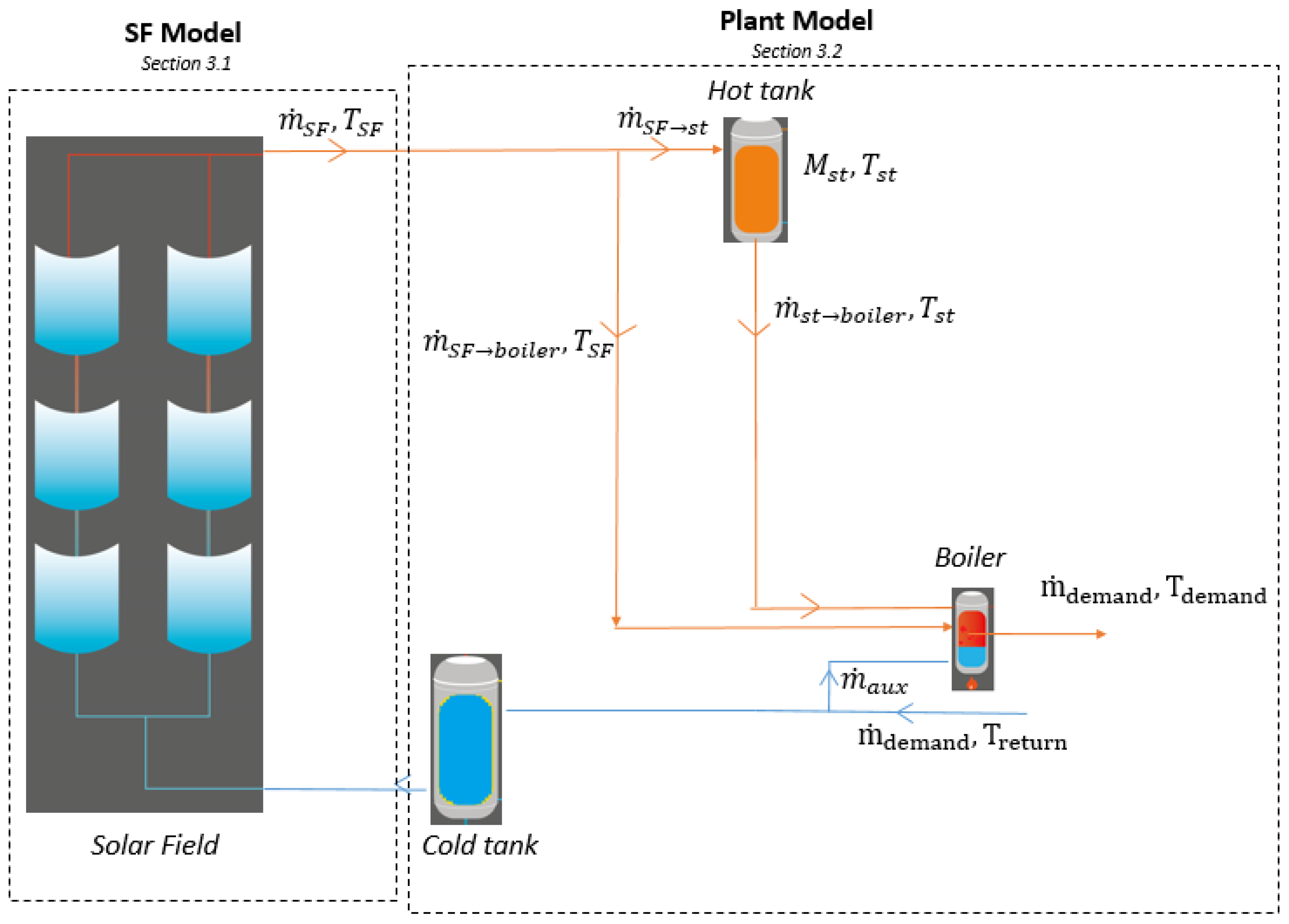
2.1.1. Schematic and System Description
2.1.2. Main Hypothesis
- Some thermal and parasitic losses are neglected: heat losses from night’s recirculation to avoid freezing, line pumping power...
- Perfectly mixed hot tank: uniform temperature in the tank.
- Heat losses’ approximation in the SF: they are classically taken as the module’s losses, with the average temperature of the SF.
- Constant fluid properties with temperature.
- Constant boiler efficiency. No limitations on the power (maximal or minimal) are considered.
- No heat losses in the cold tank: no calculations were made on the cold tank, although heat losses do happen in it as well.
- Perfect solar forecast: this hypothesis is chosen in order to exclude the influence of the forecasting model.
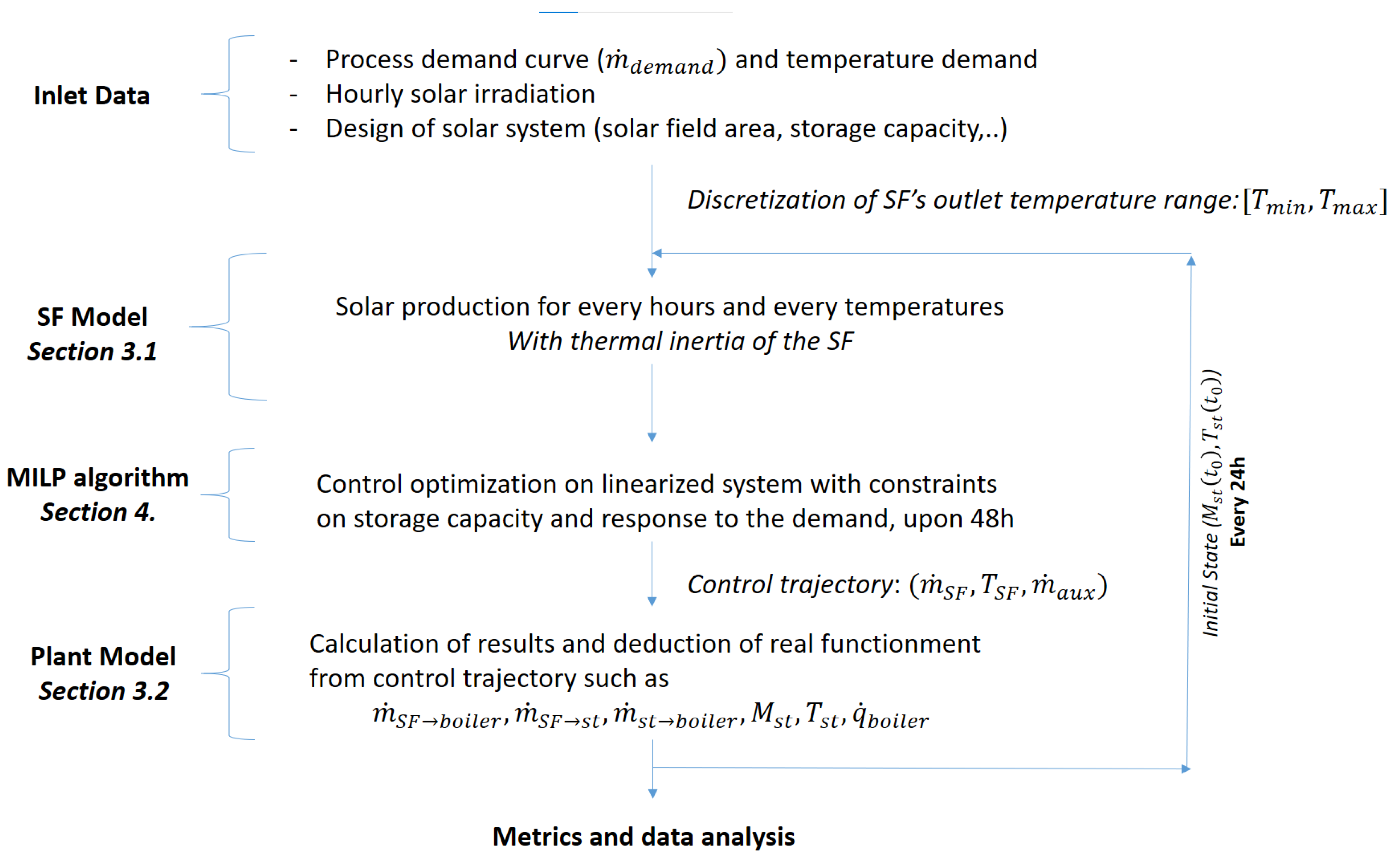
2.2. Algorithm Structure
3. Physical Model
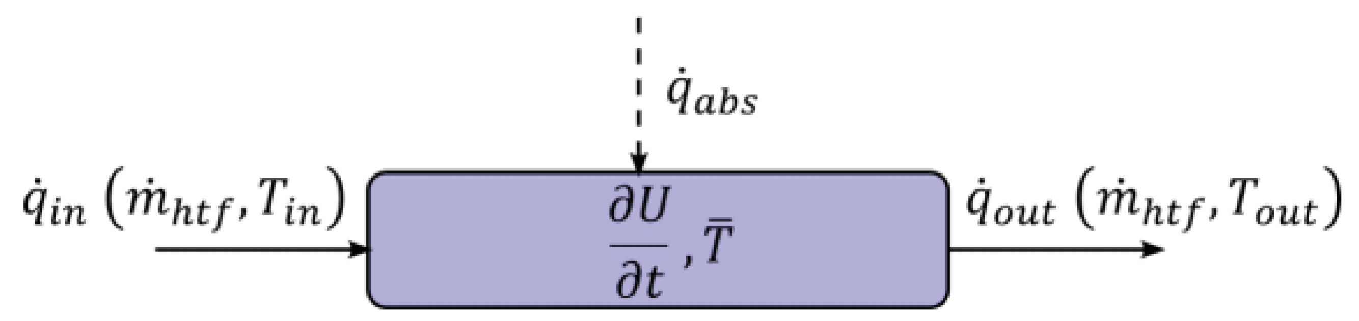
3.1. 0D Solar Field Model
- Sun position
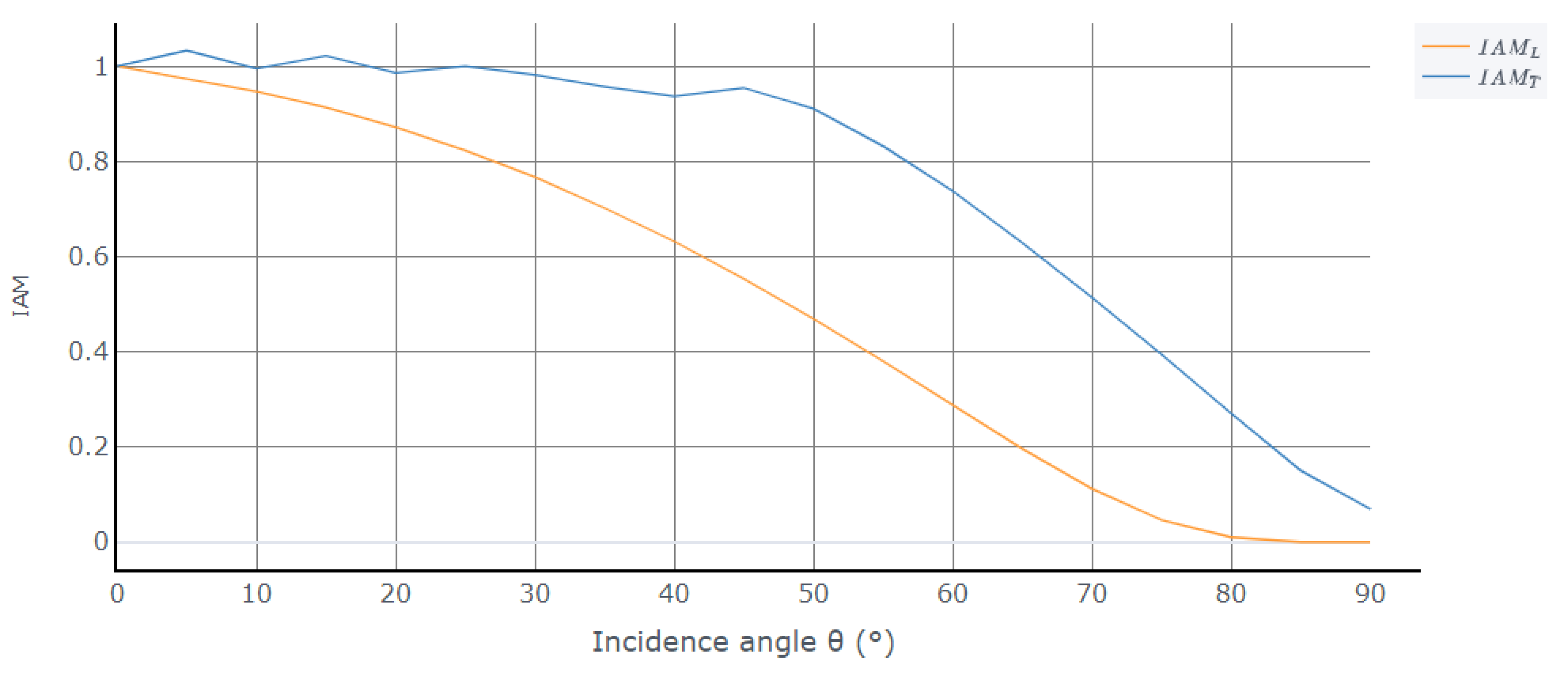
- Optical efficiency
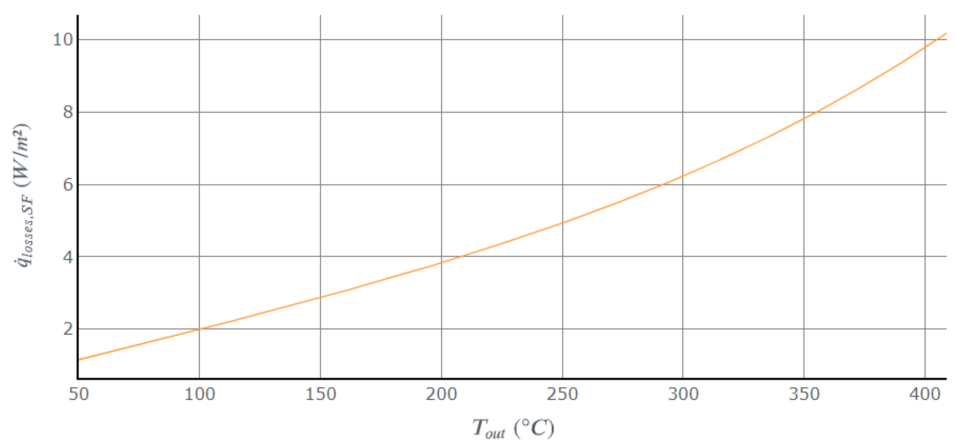
- Heat losses
- Heat from the solar field
- Mass flow rate of the SF from outlet temperature, considering inertia.
- Validation
3.2. Plant Model
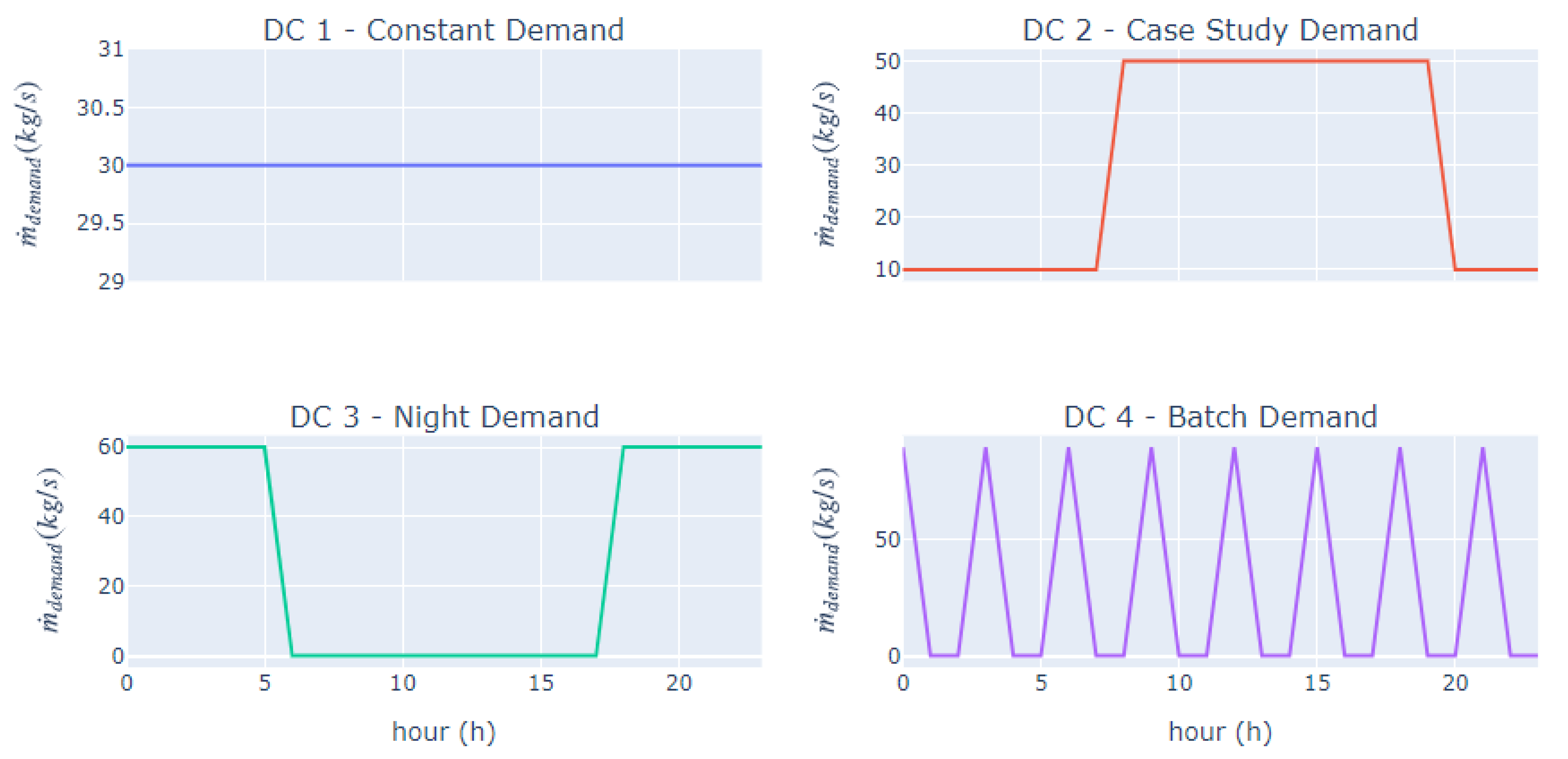
3.2.1. Mass and Mass Flow Rates Balance (Storage and Demand)
- Case 1: . Too much mass flow rate at the inlet, need to defocus. Implementation:
- Case 2: . Demand was not answered correctly, need to increase the auxiliary mass flow rate. Implementation:
3.2.2. Temperature of the Storage
3.2.3. Boiler Model
3.2.4. Plant Metrics
4. Control Models
4.1. MILP Algorithm
4.1.1. General Description of MILP Algorithm and Solver
4.1.2. Methodology: How Is the Mathematical Problem Posed
4.1.3. From Algorithm Parameters to MILP Algorithm’s Parameters
- Temperature range discretization:
- Absorbed heat from the sun, from Equation (3):
- Mass flow rate calculation:
4.1.4. From MILP Parameters to MILP Formulation
4.2. Control Models for Comparison
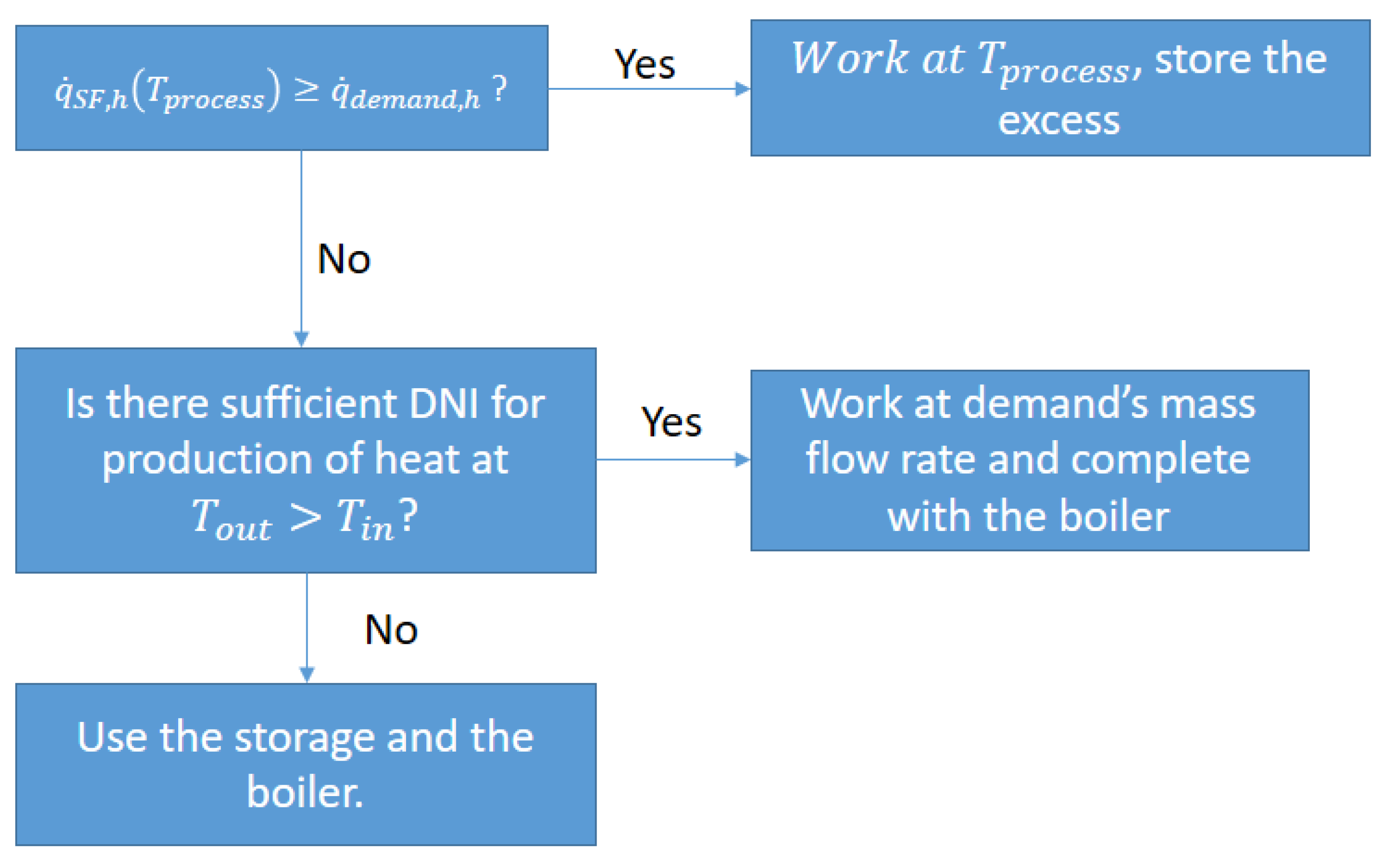
4.2.1. Control Approach 1 (CA1)
4.2.2. Control Approach 2 (CA2)
5. Case study and Results
5.1. Case Study
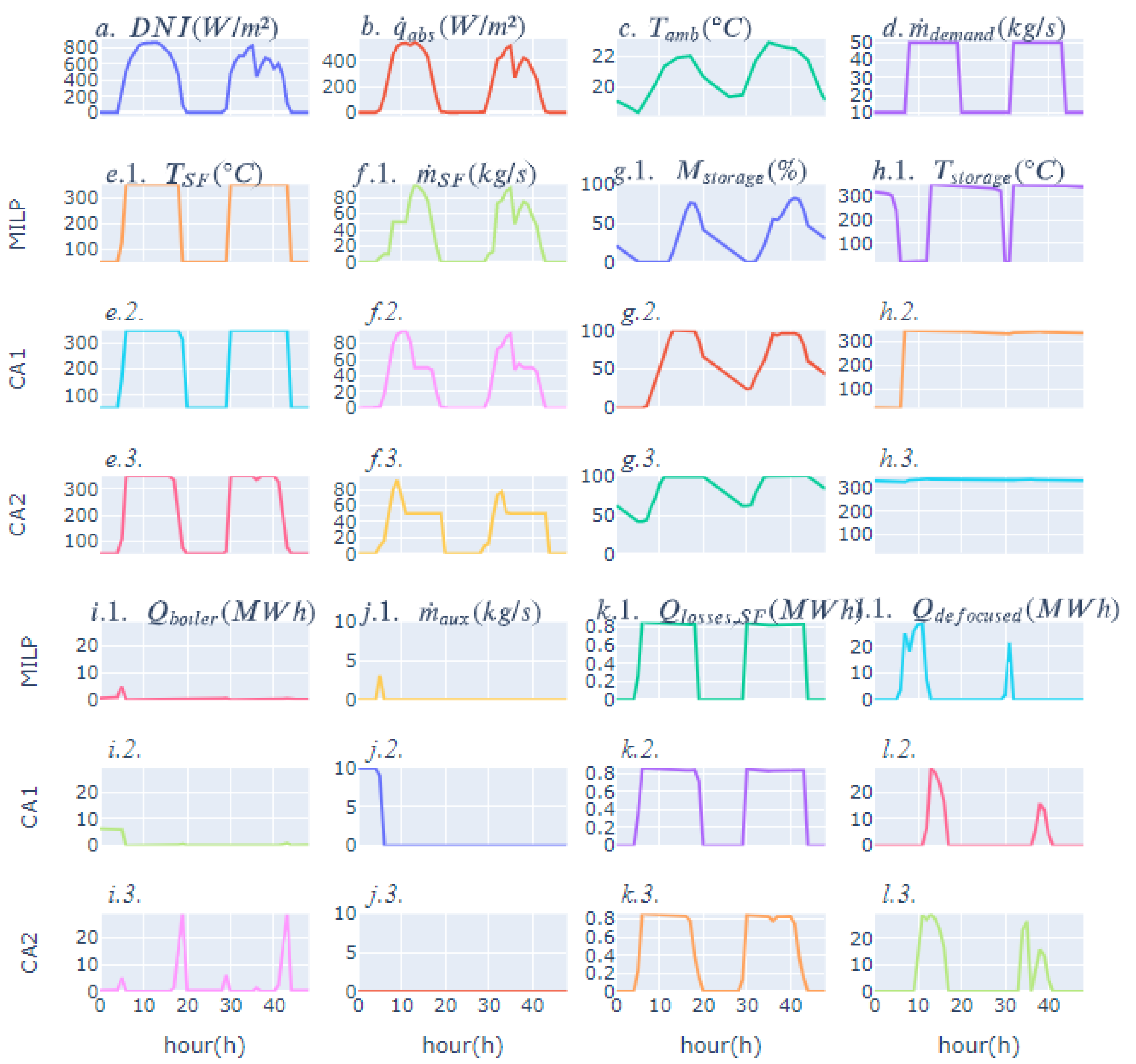
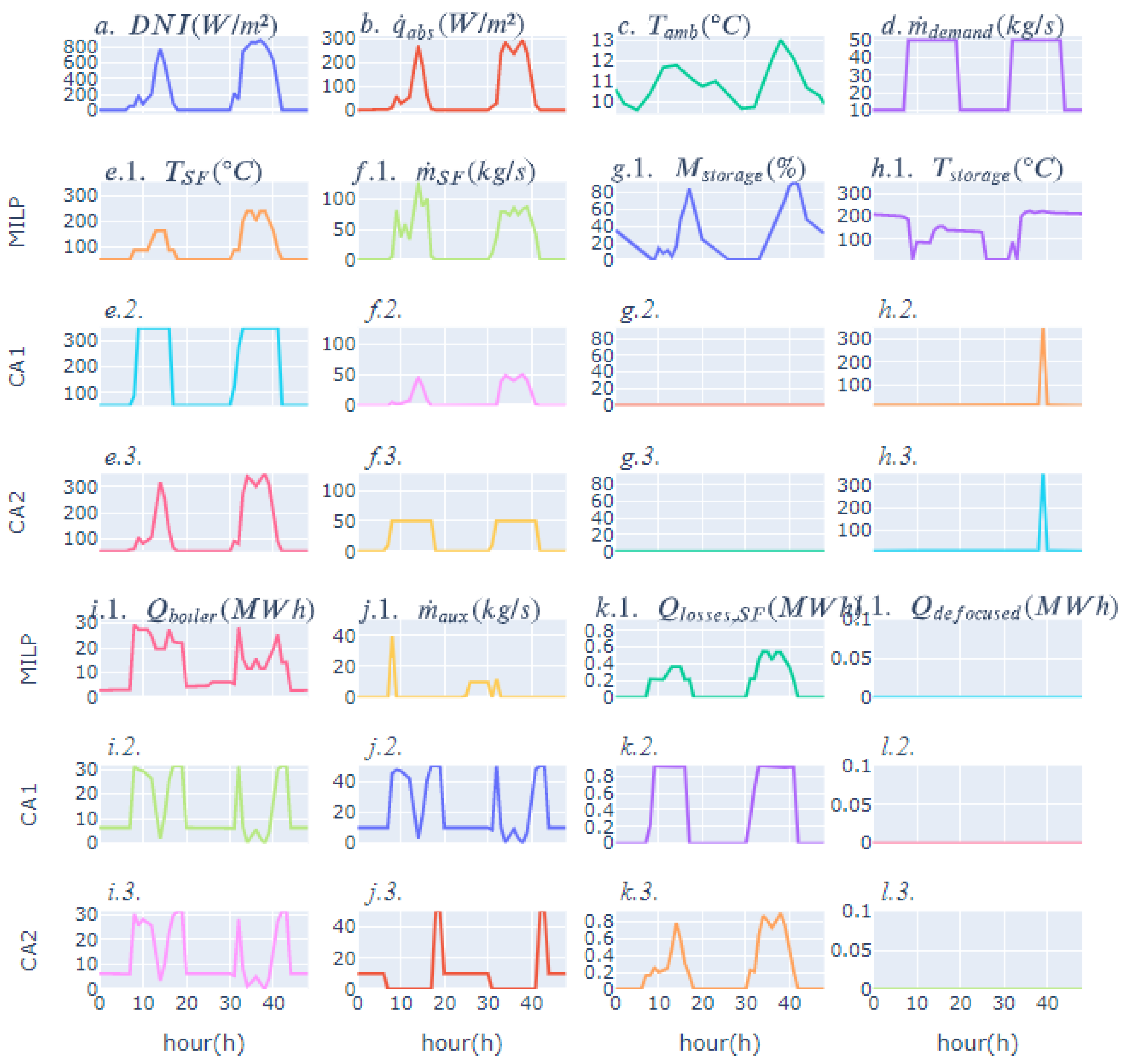
5.2. Hourly Results
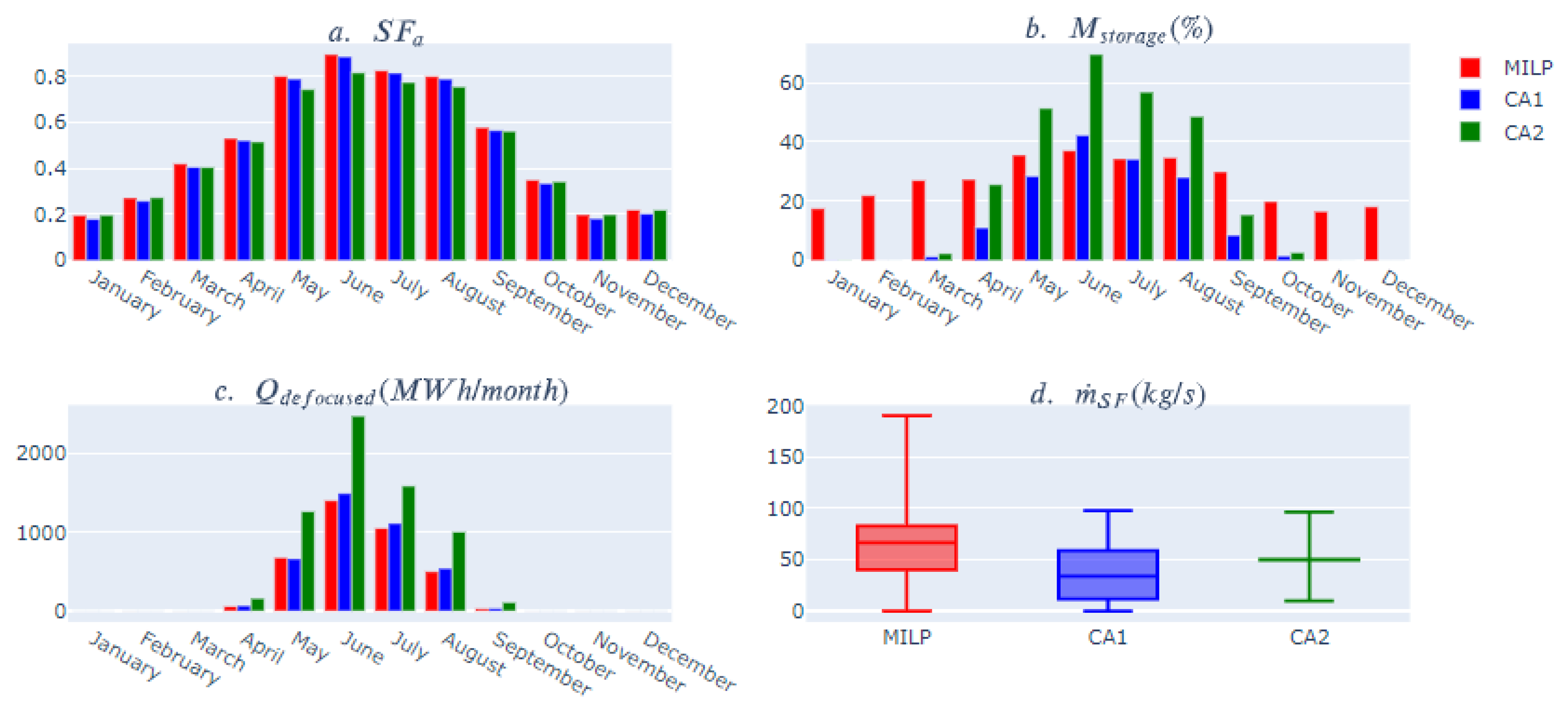
5.3. Yearly Results
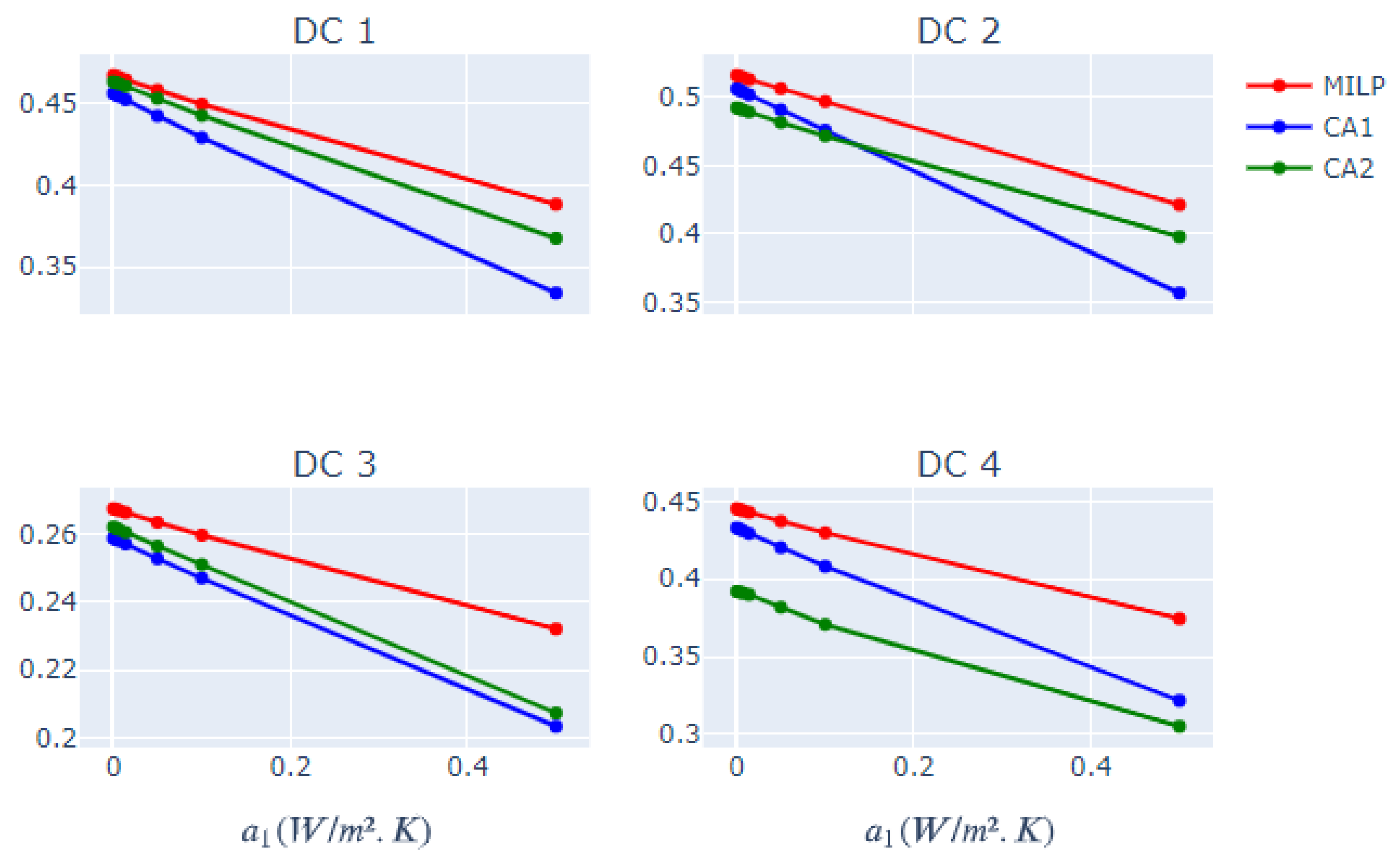
6. Sensitivity Analysis
6.1. Methodology
- -
- the number of modules in one loop is determined with the nominal mass flow rate of the module, the inlet and outlet temperature at design, under a condition of 900 W/m2:
- -
- the number of loops in parallel is determined with the solar field area necessary to answer the need with the available DNI on a user-chosen clear-sky day, the design efficiency, and the solar multiple:
- -
- the size of the storage is calculated from the number of storage hours and the average mass flow rate demand in kg/h:
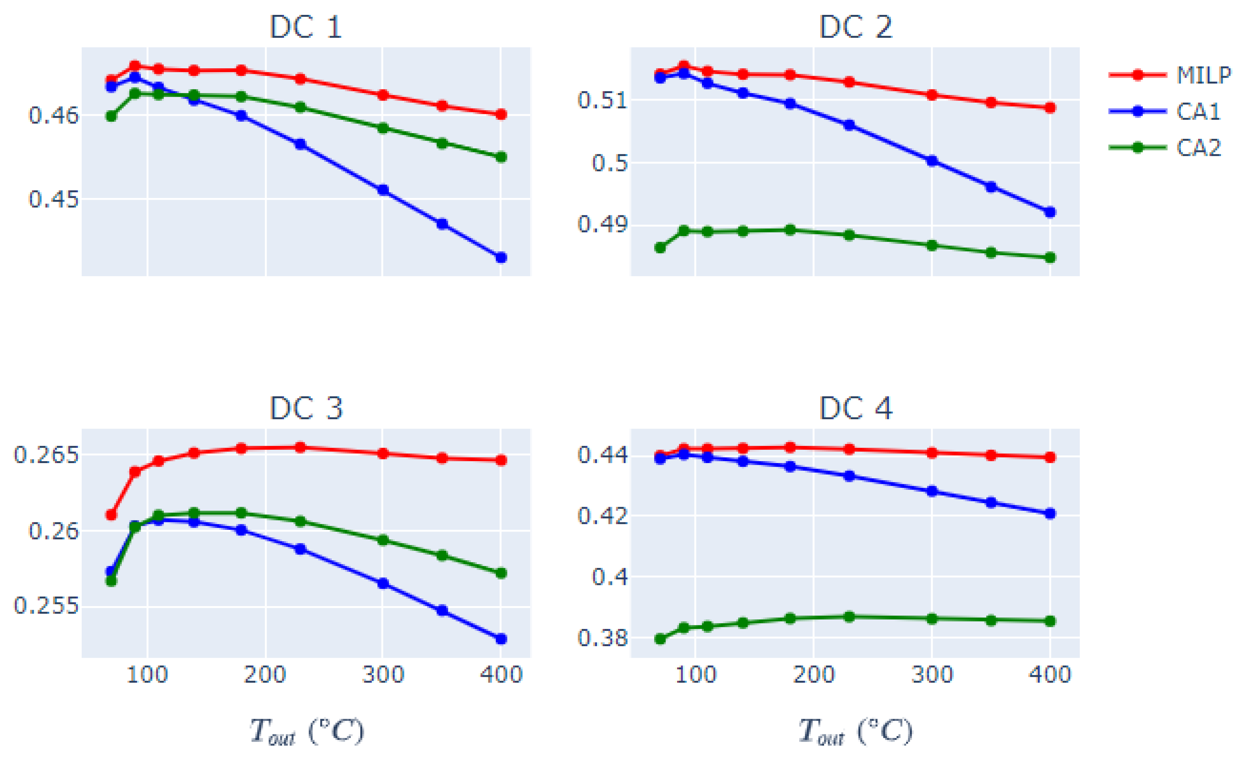
6.2. Process Temperature
6.3. Heat Losses
6.4. Other Sensibility Analyses
7. Discussion and Perspectives
8. Conclusions
Author Contributions
Funding
Institutional Review Board Statement
Informed Consent Statement
Data Availability Statement
Acknowledgments
Conflicts of Interest
Abbreviations
| Nomenclature | |
| Area (m2) | |
| ) | |
| Specific heat capacity at constant pressure (J/kg·°C) | |
| Direct Normal Irradiation (W/m2) | |
| Specific enthalpy (J/kg) | |
| IAM | Incidence Angle Modifier (-) |
| Inertia of the fluid (J/K) | |
| Mass (kg) | |
| Mass flow rate (kg/s) | |
| Integer number (-) | |
| Heat (J or Wh) | |
| Heat flux (W) | |
| Solar Fraction (-) | |
| Solar Multiple (-) | |
| Solar vector | |
| Temperature (°C) | |
| UA | Heat losses of the storage (W/K) |
| Greek Symbols | |
| Azimuth of the sun (0° North, 90° East) | |
| Efficiency | |
| Elevation of the sun (0° Horizon, 90° Zenith) | |
| Incidence angle on collector | |
| Latitude | |
| Subscripts | |
| abs | Absorbed |
| amb | Ambient |
| aux | Auxiliary |
| boiler | Boiler |
| h | Hour h |
| in | Inlet of the solar field |
| L | Longitudinal |
| opt | Optical |
| out | Outlet of the solar field |
| SF | Solar Field |
| St | Storage |
| T | Transversal |
| Flow from component x to component y | |
References
- Kumar, L.; Hasanuzzaman, M.; Rahim, N.A. Global Advancement of Solar Thermal Energy Technologies for Industrial Process Heat and Its Future Prospects: A Review. Energy Convers. Manag. 2019, 195, 885–908. [Google Scholar] [CrossRef]
- Schoeneberger, C.A.; McMillan, C.A.; Kurup, P.; Akar, S.; Margolis, R.; Masanet, E. Solar for Industrial Process Heat: A Review of Technologies, Analysis Approaches, and Potential Applications in the United States. Energy 2020, 206, 118083. [Google Scholar] [CrossRef]
- Pietruschka, D.; Fedrizzi, R.; Orioli, F.; Söll, R.; Stauss, R. Demonstration of Three Large Scale Solar Process Heat Applications with Different Solar Thermal Collector Technologies. Energy Procedia 2012, 30, 755–764. [Google Scholar] [CrossRef] [Green Version]
- IEA. IEA Task 49/IV Database for Applications of Solar Heat Integration in Industrial Processes; International Energy Agency: Paris, France, 2015. [Google Scholar]
- Wallerand, A.S.; Selviaridis, A.; Ashouri, A.; Maréchal, F. Targeting Optimal Design and Operation of Solar Heated Industrial Processes: A MILP Formulation. Energy Procedia 2016, 91, 668–680. [Google Scholar] [CrossRef] [Green Version]
- Omu, A.; Hsieh, S.; Orehounig, K. Mixed Integer Linear Programming for the Design of Solar Thermal Energy Systems with Short-Term Storage. Appl. Energy 2016, 180, 313–326. [Google Scholar] [CrossRef]
- Tilahun, F.B.; Bhandari, R.; Mamo, M. Design Optimization and Control Approach for a Solar-Augmented Industrial Heating. Energy 2019, 179, 186–198. [Google Scholar] [CrossRef]
- Fitsum, B.T.; Ramchandra, B.; Menegesha, M. Design Optimization and Demand Side Management of a Solar-Assisted Industrial Heating Using Agent-Based Modelling (ABM): Methodology and Case Study. E3S Web Conf. 2018, 64, 02001. [Google Scholar] [CrossRef]
- Ghazouani, M.; Bouya, M.; Benaissa, M. Thermo-Economic and Exergy Analysis and Optimization of Small PTC Collectors for Solar Heat Integration in Industrial Processes. Renew. Energy 2020, 152, 984–998. [Google Scholar] [CrossRef]
- Wagner, M.J.; Hamilton, W.T.; Newman, A.; Dent, J.; Diep, C.; Braun, R. Optimizing Dispatch for a Concentrated Solar Power Tower. Solar Energy 2018, 174, 1198–1211. [Google Scholar] [CrossRef]
- Vasallo, M.J.; Bravo, J.M. A Novel Two-Model Based Approach for Optimal Scheduling in CSP Plants. Solar Energy 2016, 126, 73–92. [Google Scholar] [CrossRef]
- He, G.; Chen, Q.; Kang, C.; Xia, Q. Optimal Offering Strategy for Concentrating Solar Power Plants in Joint Energy, Reserve and Regulation Markets. IEEE Trans. Sustain. Energy 2016, 7, 1245–1254. [Google Scholar] [CrossRef]
- Petrollese, M.; Cocco, D.; Cau, G.; Cogliani, E. Comparison of Three Different Approaches for the Optimization of the CSP Plant Scheduling. Solar Energy 2017, 150, 463–476. [Google Scholar] [CrossRef]
- Dowling, A.W.; Zheng, T.; Zavala, V.M. A Decomposition Algorithm for Simultaneous Scheduling and Control of CSP Systems. AIChE J. 2018, 64, 2408–2417. [Google Scholar] [CrossRef]
- Pousinho, H.M.I.; Contreras, J.; Pinson, P.; Mendes, V.M.F. Robust Optimisation for Self-Scheduling and Bidding Strategies of Hybrid CSP–Fossil Power Plants. Int. J. Electr. Power Energy Syst. 2015, 67, 639–650. [Google Scholar] [CrossRef]
- Pousinho, H.M.I.; Silva, H.; Mendes, V.M.F.; Collares-Pereira, M.; Pereira Cabrita, C. Self-Scheduling for Energy and Spinning Reserve of Wind/CSP Plants by a MILP Approach. Energy 2014, 78, 524–534. [Google Scholar] [CrossRef]
- Yang, Y.; Guo, S.; Liu, D.; Li, R.; Chu, Y. Operation Optimization Strategy for Wind-Concentrated Solar Power Hybrid Power Generation System. Energy Convers. Manag. 2018, 160, 243–250. [Google Scholar] [CrossRef]
- Zhao, S.; Fang, Y.; Wei, Z. Stochastic Optimal Dispatch of Integrating Concentrating Solar Power Plants with Wind Farms. Int. J. Electr. Power Energy Syst. 2019, 109, 575–583. [Google Scholar] [CrossRef]
- Hamilton, W.T.; Husted, M.A.; Newman, A.M.; Braun, R.J.; Wagner, M.J. Dispatch Optimization of Concentrating Solar Power with Utility-Scale Photovoltaics. Optim. Eng. 2020, 21, 335–369. [Google Scholar] [CrossRef]
- Rashid, K.; Safdarnejad, S.M.; Powell, K.M. Process Intensification of Solar Thermal Power Using Hybridization, Flexible Heat Integration, and Real-Time Optimization. Chem. Eng. Process. Process. Intensif. 2019, 139, 155–171. [Google Scholar] [CrossRef] [Green Version]
- Ellingwood, K.; Mohammadi, K.; Powell, K. A Novel Means to Flexibly Operate a Hybrid Concentrated Solar Power Plant and Improve Operation during Non-Ideal Direct Normal Irradiation Conditions. Energy Convers. Manag. 2020, 203, 112275. [Google Scholar] [CrossRef]
- Wirtz, M. Temperature Control in 5th Generation District Heating and Cooling Networks: An MILP-Based Operation Optimization. Appl. Energy 2021, 288, 116608. [Google Scholar] [CrossRef]
- Industrial Solar LF-11. Available online: https://www.industrial-solar.de/technologies/fresnel-collector/ (accessed on 16 June 2021).
- Blanco-Muriel, M.; Alarcón-Padilla, D.C.; López-Moratalla, T.; Lara-Coira, M. Computing the Solar Vector. Solar Energy 2001, 70, 431–441. [Google Scholar] [CrossRef]
- Morin, G.; Dersch, J.; Platzer, W.; Eck, M.; Häberle, A. Comparison of Linear Fresnel and Parabolic Trough Collector Power Plants. Solar Energy 2012, 86, 1–12. [Google Scholar] [CrossRef]
- Wagner, M.J.; Gilman, P. Technical Manual for the SAM Physical Trough Model; NREL/TP-5500-51825; National Renewable Energy Laboratory: Golden, CO, USA, 2011; p. 1016437. [Google Scholar]
- System Advisor Model Version 2020.11.29 (SAM 2020.11.29). National Renewable Energy Laboratory: Golden, CO, USA. Available online: https://sam.nrel.gov/ (accessed on 16 June 2021).
- Rao, S.S. Engineering Optimization: Theory and Practice, 4th ed.; John Wiley & Sons: Hoboken, NJ, USA, 2009; ISBN 978-0-470-18352-6. [Google Scholar]
- Coin-OR Coin-OR CBC MIP Solver; Johnjforrest, S.; Vigerske, H.G.; Santos, T.; Ralphs, L.; Hafer, B.; Kristjansson; Jpfasano; EdwinStraver; Lubin, M.; et al. Coin-or/Cbc: Version 2.10.5. Available online: https://github.com/coin-or/Cbc (accessed on 16 June 2021).
- EU SCIENCE HUB. Photovoltaic Geographical Information System (PVGIS); EU SCIENCE HUB: Ispra, Italy, 2019; Available online: https://ec.europa.eu/jrc/en/pvgis (accessed on 16 June 2021).
- Kamerling, S.; Vuillerme, V.; Rodat, S. Data for Solar Field Output Temperature Optimization Using a MILP Algorithm and a 0D Model in the Case of a Hybrid Concentrated Solar Thermal Power Plant for SHIP Applications. Available online: https://doi.org/10.5281/zenodo.5006230 (accessed on 16 June 2021).


| Variable | Value (Unit) | Description |
|---|---|---|
| 41.117° | Latitude | |
| 451 MWh/day | Daily heat demand | |
| 350 °C | Process temperature | |
| 50 °C | Return temperature | |
| 0.6 | Design efficiency (defined in Section 4.1) | |
| SM | 1.5 | Solar Multiple (defined in Section 4.1) |
| 113,367 m2 | Solar field area | |
| 31 | Number of modules in one loop | |
| 159 | Number of loops | |
| 8 h | Storage hours | |
| 864 t | Tank capacity | |
| 570 W/K | Heat losses of the storage |
Publisher’s Note: MDPI stays neutral with regard to jurisdictional claims in published maps and institutional affiliations. |
© 2021 by the authors. Licensee MDPI, Basel, Switzerland. This article is an open access article distributed under the terms and conditions of the Creative Commons Attribution (CC BY) license (https://creativecommons.org/licenses/by/4.0/).
Share and Cite
Kamerling, S.; Vuillerme, V.; Rodat, S. Solar Field Output Temperature Optimization Using a MILP Algorithm and a 0D Model in the Case of a Hybrid Concentrated Solar Thermal Power Plant for SHIP Applications. Energies 2021, 14, 3731. https://doi.org/10.3390/en14133731
Kamerling S, Vuillerme V, Rodat S. Solar Field Output Temperature Optimization Using a MILP Algorithm and a 0D Model in the Case of a Hybrid Concentrated Solar Thermal Power Plant for SHIP Applications. Energies. 2021; 14(13):3731. https://doi.org/10.3390/en14133731
Chicago/Turabian StyleKamerling, Simon, Valéry Vuillerme, and Sylvain Rodat. 2021. "Solar Field Output Temperature Optimization Using a MILP Algorithm and a 0D Model in the Case of a Hybrid Concentrated Solar Thermal Power Plant for SHIP Applications" Energies 14, no. 13: 3731. https://doi.org/10.3390/en14133731
APA StyleKamerling, S., Vuillerme, V., & Rodat, S. (2021). Solar Field Output Temperature Optimization Using a MILP Algorithm and a 0D Model in the Case of a Hybrid Concentrated Solar Thermal Power Plant for SHIP Applications. Energies, 14(13), 3731. https://doi.org/10.3390/en14133731