
How Can Floor Covering Influence Buildings’ Demand Flexibility?


Abstract
1. Introduction
2. Methodology
2.1. Description of EnergyPlus
2.2. Description of the DOE’s Reference Small Office Building Model
2.3. Description of Simulated Cases
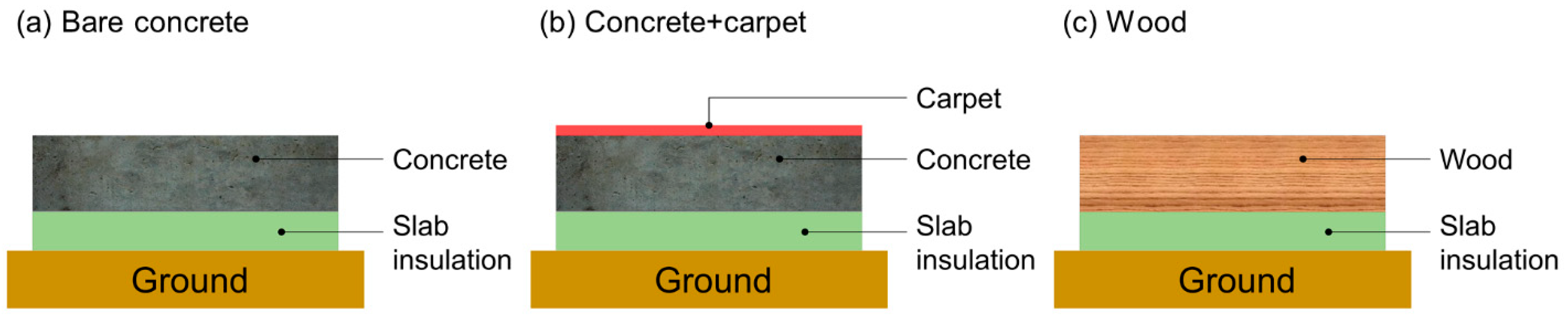
2.4. Description of Floor Configurations
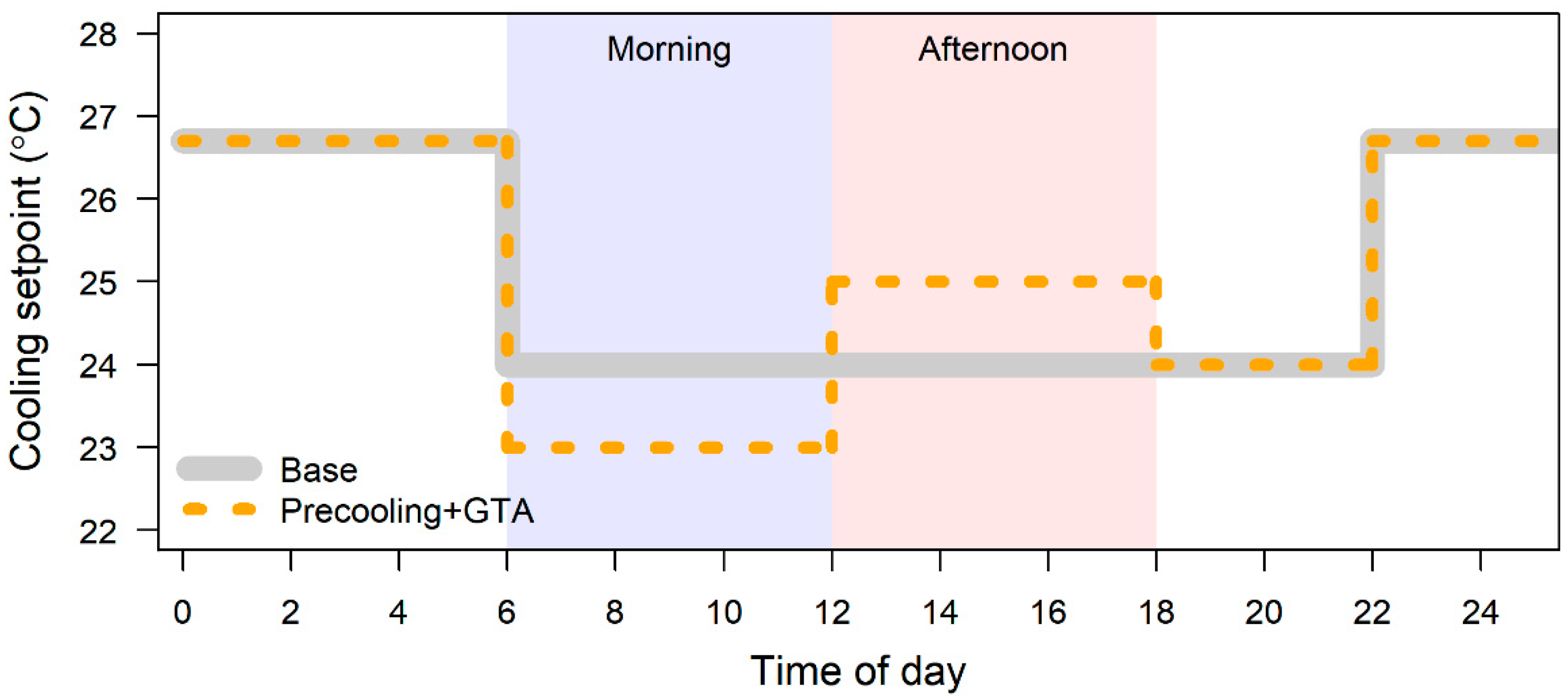
2.5. Description of Cooling Strategies
2.6. Evalation Criteria for Demand Flexibility
3. Sensitivity Analysis
3.1. Sensitivity of Carpet-Covered Area to Demand Flexibility
3.2. Sensitivity of Temperature Adjustment Depth to Demand Flexibility
4. Results and Discussion
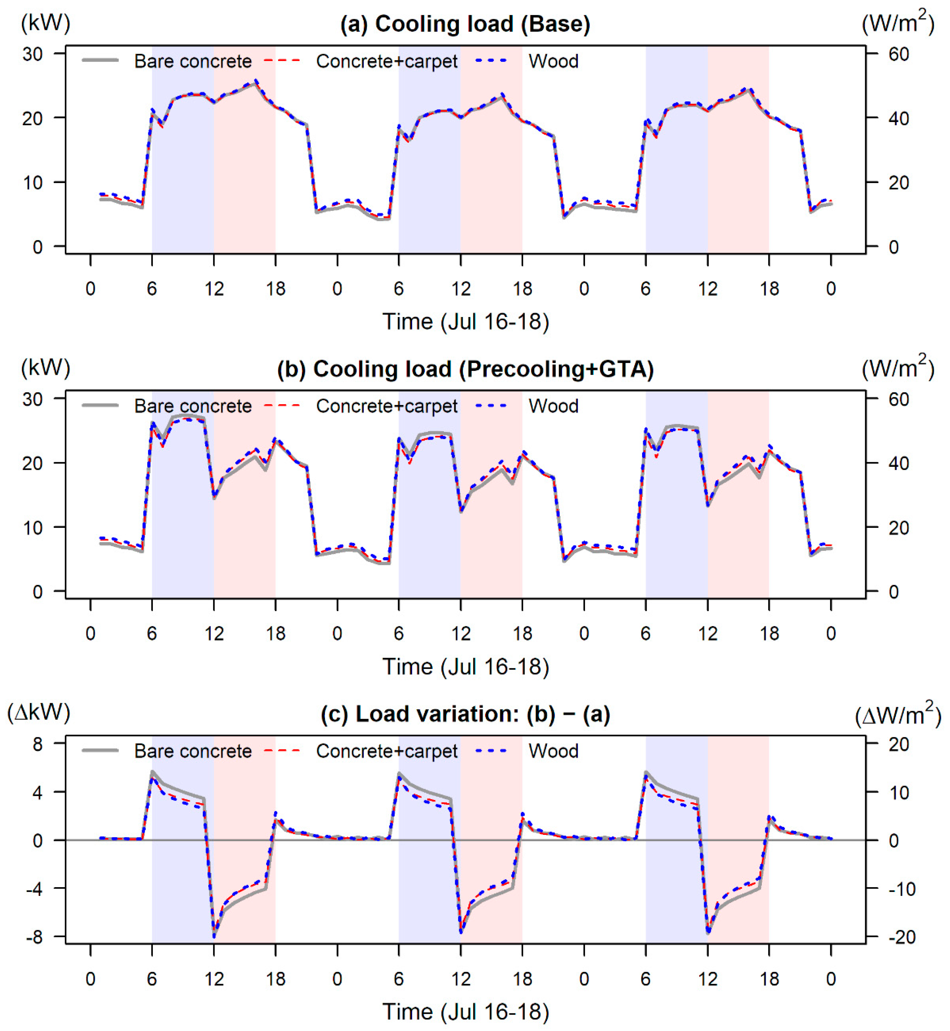
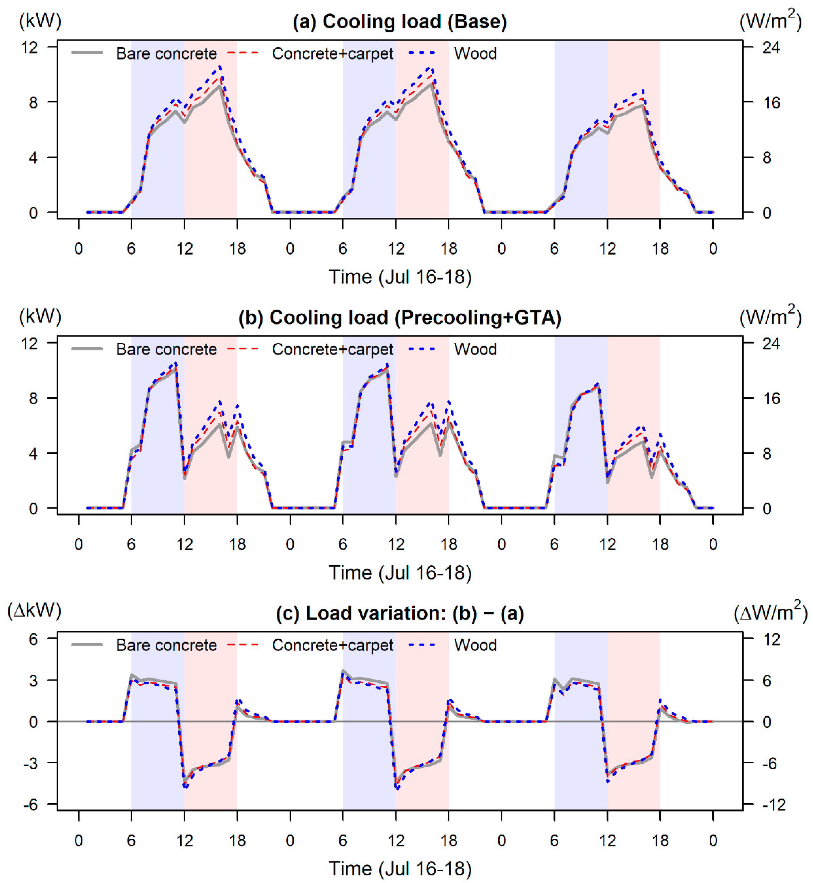
4.1. Hourly Cooling Load Profiles
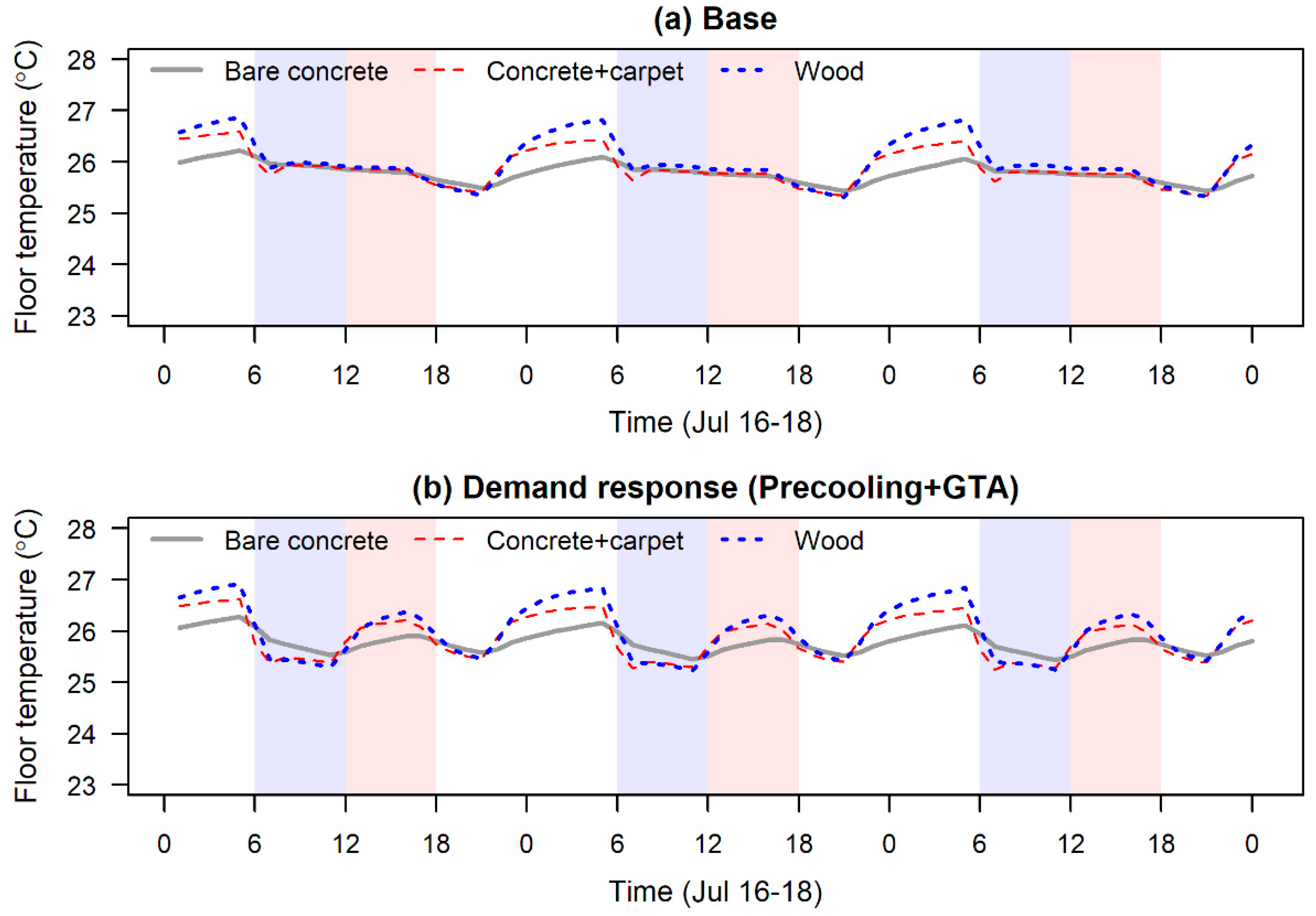
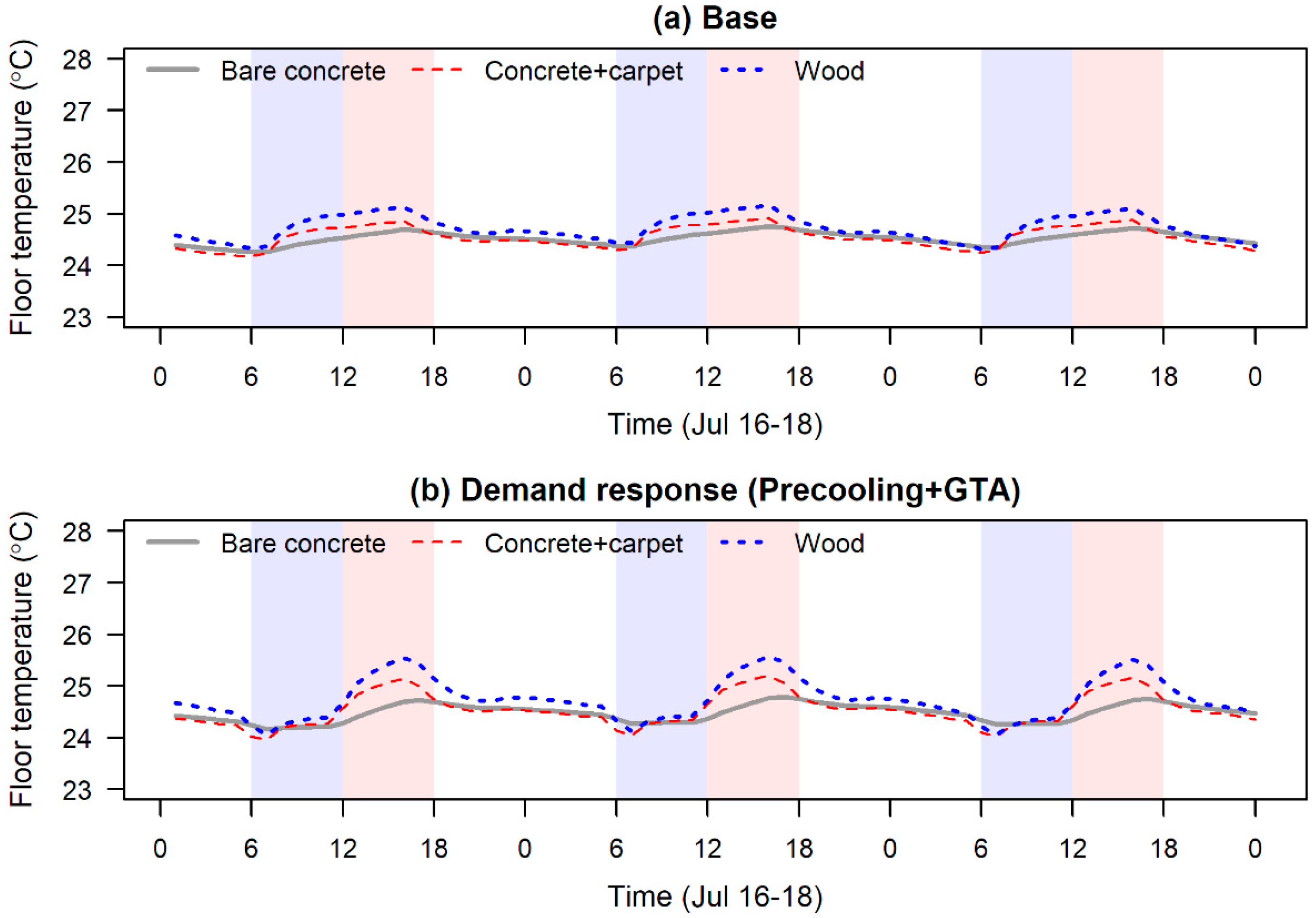
4.2. Floor Surface Temperature
4.3. Daily Peak Cooling Load
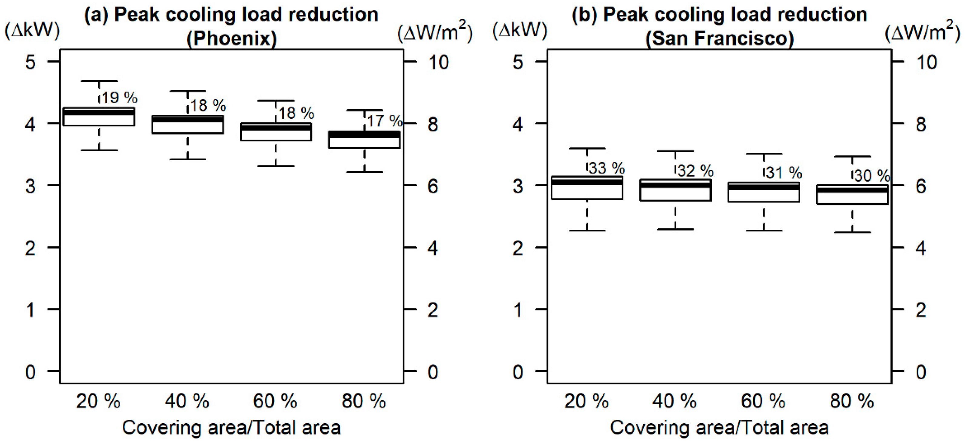
4.4. Sensitivity of Floor Covering Area to Demand Flexibility
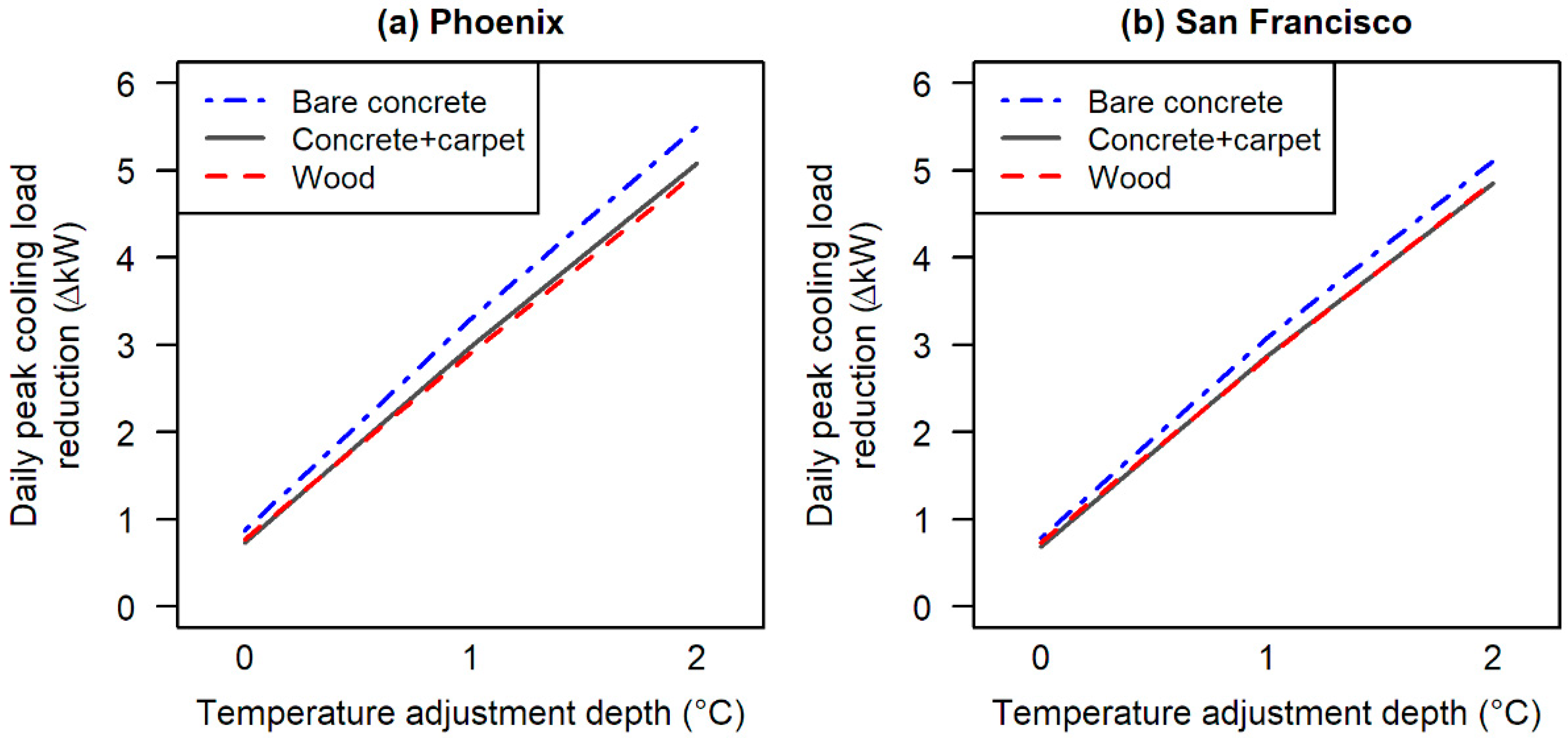
4.5. Sensitivity of GTA Depth to Demand Flexibility
5. Further Discussion about Convective and Radiant Fractions of Internal Heat Gains
6. Limitations and Future Research
7. Conclusions
Supplementary Materials
Author Contributions
Funding
Institutional Review Board Statement
Informed Consent Statement
Acknowledgments
Conflicts of Interest
References
- Denholm, P.; Hand, M. Grid flexibility and storage required to achieve very high penetration of variable renewable electricity. Energy Policy 2011, 39, 1817–1830. [Google Scholar] [CrossRef]
- Sun, Y.; Wachche, S.; Mills, A.; Ma, O. 2018 Renewable Energy Grid Integration Data Book; National Renewable Energy Laboratory: Golden, CO, USA, 2020; p. 124. [Google Scholar]
- Wang, Q.; Hodge, B.-M. Enhancing Power System Operational Flexibility with Flexible Ramping Products: A Review. IEEE Trans. Ind. Inform. 2017, 13, 1652–1664. [Google Scholar] [CrossRef]
- Kathan, D.; Daly, C.; Eversole, E.; Farinella, M.; Gadani, J.; Irwin, R.; Lankford, C.; Pan, A.; Switzer, C.; Wight, D. National Action Plan on Demand Response; Federal Energy Regulatory Commission: Washington, DC, USA, 2010; p. 118. [Google Scholar]
- Neukomm, M.; Nubbe, V.; Fares, R. Grid-Interactive Efficient Buildings: Overview; U.S. Department of Energy: Washington, DC, USA, 2019; p. 36. [Google Scholar]
- U.S. Energy Information Administration Electricity Data. Available online: https://www.eia.gov/electricity/monthly/epm_table_grapher.php?t=epmt_5_01 (accessed on 7 August 2020).
- Xu, P.; Haves, P. Case Study of Demand Shifting with Thermal Mass in Two Large Commercial Buildings. ASHRAE Trans. 2006, 112, 572–580. [Google Scholar]
- Lee, K.-H.; Braun, J.E. Model-based demand-limiting control of building thermal mass. Build. Environ. 2008, 43, 1633–1646. [Google Scholar] [CrossRef]
- Braun, J. Reducing Energy Costs and Peak Electrical Demand. ASHRAE Trans. 1990, 876–888. [Google Scholar]
- Aste, N.; Leonforte, F.; Manfren, M.; Mazzon, M. Thermal inertia and energy efficiency–Parametric simulation assessment on a calibrated case study. Appl. Energy 2015, 145, 111–123. [Google Scholar] [CrossRef]
- Henze, G.P.; Le, T.H.; Florita, A.; Felsmann, C. Sensitivity Analysis of Optimal Building Thermal Mass Control. J. Sol. Energy Eng. 2007, 129, 473–485. [Google Scholar] [CrossRef]
- Turner, W.; Walker, I.; Roux, J. Peak load reductions: Electric load shifting with mechanical pre-cooling of residential buildings with low thermal mass. Energy 2015, 82, 1057–1067. [Google Scholar] [CrossRef]
- Høseggen, R.; Mathisen, H.; Hanssen, S. The effect of suspended ceilings on energy performance and thermal comfort. Energy Build. 2009, 41, 234–245. [Google Scholar] [CrossRef]
- Raftery, P.; Lee, E.; Webster, T.; Hoyt, T.; Bauman, F. Effects of furniture and contents on peak cooling load. Energy Build. 2014, 85, 445–457. [Google Scholar] [CrossRef]
- Wolisz, H.; Kull, T.M.; Streblow, R.; Müller, D. The Effect of Furniture and Floor Covering Upon Dynamic Thermal Building Simulations. Energy Procedia 2015, 78, 2154–2159. [Google Scholar] [CrossRef]
- Gerke, B.; Zhang, C.; Satchwell, A.; Murthy, S.; Piette, M.; Present, E.; Wilson, E.; Speake, A.; Adhikari, R. Modeling the In-teraction Between Energy Efficiency and Demand Response on Regional Grid Scales. In Proceedings of the 2020 ACEEE Summer Study on Energy Efficiency in Buildings, ACEEE, Pacific Grove, CA, USA, 17–21 August 2020. [Google Scholar]
- Rabl, A.; Norford, L.K. Peak load reduction by preconditioning buildings at night. Int. J. Energy Res. 1991, 15, 781–798. [Google Scholar] [CrossRef]
- Kintner-Meyer, M.; Emery, A. Optimal control of an HVAC system using cold storage and building thermal capacitance. Energy Build. 1995, 23, 19–31. [Google Scholar] [CrossRef]
- Becker, R.; Paciuk, M. Inter-related effects of cooling strategies and building features on energy performance of office buildings. Energy Build. 2002, 34, 25–31. [Google Scholar] [CrossRef]
- Zhou, G.; Krarti, M.; Henze, G.P. Parametric Analysis of Active and Passive Building Thermal Storage Utilization*. J. Sol. Energy Eng. 2005, 127, 37–46. [Google Scholar] [CrossRef]
- Yang, L.; Li, Y. Cooling load reduction by using thermal mass and night ventilation. Energy Build. 2008, 40, 2052–2058. [Google Scholar] [CrossRef]
- Chen, Y.; Chen, Z.; Xu, P.; Li, W.; Sha, H.; Yang, Z.; Li, G.; Hu, C. Quantification of electricity flexibility in demand response: Office building case study. Energy 2019, 188, 116054. [Google Scholar] [CrossRef]
- Panão, M.J.O.; Mateus, N.M.; Da Graça, G.C. Measured and modeled performance of internal mass as a thermal energy battery for energy flexible residential buildings. Appl. Energy 2019, 239, 252–267. [Google Scholar] [CrossRef]
- Zhang, Y.; Korolija, I. Performing Complex Parametric Simulations with JEPlus. In Proceedings of the SET 2010: 9th Interna-tional Conference on Sustainable Energy Technologies, Shanghai, China, 24–27 August 2010; p. 6. [Google Scholar]
- U.S. Department of Energy. EnergyPlus. Available online: https://energyplus.net/ (accessed on 10 August 2020).
- Chantrasrisalai, C.; Ghatti, V.; Fisher, D.E.; Scheatzle, D.G. Experimental Validation of the EnergyPlus Low-Temperature Radiant Simulation. ASHRAE Trans. 2003, 109, 614–623. [Google Scholar]
- Tabares-Velasco, P.C.; Christensen, C.; Bianchi, M. Verification and validation of EnergyPlus phase change material model for opaque wall assemblies. Build. Environ. 2012, 54, 186–196. [Google Scholar] [CrossRef]
- Mateus, N.M.; Pinto, A.; da Graca, G.C. Validation of EnergyPlus thermal simulation of a double skin naturally and mechanically ventilated test cell. Energy Build. 2014, 75, 511–522. [Google Scholar] [CrossRef]
- Hong, T.; Sun, K.; Zhang, R.; Hinokuma, R.; Kasahara, S.; Yura, Y. Development and validation of a new variable refrigerant flow system model in EnergyPlus. Energy Build. 2016, 117, 399–411. [Google Scholar] [CrossRef]
- U.S. Energy Information Administration, Commercial Buildings Energy Consumption Survey (CBECS). Available online: https://www.eia.gov/consumption/commercial/data/2012/c&e/cfm/c11.php (accessed on 19 February 2019).
- Deru, M.; Field, K.; Studer, D.; Benne, K.; Griffith, B.; Torcellini, P.; Liu, B.; Halverson, M.; Winiarski, D.; Rosenberg, M.; et al. US Department of Energy Commercial Reference Building Models of the National Building Stock; National Renewable Energy Laboratory: Golden, CO, USA, 2011. [Google Scholar]
- International Code Council. 2012 International Energy Conservation Code; International Code Council: Country Club Hills, IL, USA, 2011; ISBN 978-1-60983-058-8. [Google Scholar]
- Wilcox, S.; Marion, W. Users Manual for TMY3 Data Sets; National Renewable Energy Laboratory: Golden, CO, USA, 2008; p. 58. [Google Scholar]
- Integrated Environmental Solutions Ltd, Table 6 Thermal Conductivity, Specific Heat Capacity and Density. Available online: https://help.iesve.com/ve2018/table_6_thermal_conductivity__specific_heat_capacity_and_density.htm (accessed on 6 October 2020).
- U.S. Department of Energy. Energyplus. Engineering Reference; Ernest Orlando Lawrence Berkeley National Laboratory: Berkeley, CA, USA, 2019. [Google Scholar]
- Yin, R.; Ghatikar, G.; Piette, M. Big-Data Analytics for Electric Grid and Demand-Side Management; Office of Scientific and Technical Information (OSTI): Berkeley, CA, USA, 2019; p. 57. [Google Scholar]
- PG&E, Time-of-Use Rate Plans. Available online: https://www.pge.com/en_US/business/rate-plans/rate-plans/time-of-use/time-of-use.page? (accessed on 10 October 2017).
- Ahn, H.; Freihaut, J.D.; Rim, D. Economic feasibility of combined cooling, heating, and power (CCHP) systems considering electricity standby tariffs. Energy 2019, 169, 420–432. [Google Scholar] [CrossRef]
- Zhu, L.; Hurt, R.; Correia, D.; Boehm, R. Detailed energy saving performance analyses on thermal mass walls demonstrated in a zero energy house. Energy Build. 2009, 41, 303–310. [Google Scholar] [CrossRef]
- Ghoreishi, A.H.; Ali, M.M. Parametric study of thermal mass property of concrete buildings in US climate zones. Arch. Sci. Rev. 2013, 56, 103–117. [Google Scholar] [CrossRef]
- Tsilingiris, P. On the thermal time constant of structural walls. Appl. Therm. Eng. 2004, 24, 743–757. [Google Scholar] [CrossRef]
- Yin, R.; Kara, E.C.; Li, Y.; DeForest, N.; Wang, K.; Yong, T.; Stadler, M. Quantifying flexibility of commercial and residential loads for demand response using setpoint changes. Appl. Energy 2016, 177, 149–164. [Google Scholar] [CrossRef]
- ASHRAE. 2017 ASHRAE Handbook-Fundamentals; American Society of Heating Refrigerating and Air-Conditioning Engineers, Inc.: Atlanta, GA, USA, 2017; ISBN 978-1-939200-57-0. [Google Scholar]
- Kim, D.; Braun, J.; Cliff, E.; Borggaard, J. Development, validation and application of a coupled reduced-order CFD model for building control applications. Build. Environ. 2015, 93, 97–111. [Google Scholar] [CrossRef]
- Ahn, H.; Rim, D.; Lo, L.J. Ventilation and energy performance of partitioned indoor spaces under mixing and displacement ventilation. Build. Simul. 2017, 11, 561–574. [Google Scholar] [CrossRef]
- Korkas, C.D.; Baldi, S.; Michailidis, I.; Kosmatopoulos, E.B. Occupancy-based demand response and thermal comfort optimization in microgrids with renewable energy sources and energy storage. Appl. Energy 2016, 163, 93–104. [Google Scholar] [CrossRef]
- Baldi, S.; Korkas, C.D.; Lv, M.; Kosmatopoulos, E.B. Automating occupant-building interaction via smart zoning of thermostatic loads: A switched self-tuning approach. Appl. Energy 2018, 231, 1246–1258. [Google Scholar] [CrossRef]


| Reference | Method | Building Type | Demand Response | Thermal Mass |
|---|---|---|---|---|
| Braun (1990) [9] | Simulation | Single-zone building | Precooling | Floor, exterior and partition walls, and ceiling |
| Rabl and Norford (1991) [17] | Simulation | Multi-story office building | Night ventilation | Floor, walls, and ceiling |
| Kintner-Meyer and Emery (1995) [18] | Simulation | Multi-story office building | Precooling | Floor, exterior walls, and ceiling |
| Becker and Paciuk (2002) [19] | Simulation | Multi-story office building | Precooling and night ventilation | Floor, exterior, interior, and partition walls |
| Zhou et al. (2005) [20] | Simulation | Multi-story office building | Precooling and night ventilation | Floor, exterior walls, roof, and ceiling |
| Xu and Haves (2006) [7] | Measurement and simulation | Multi-story office building | Precooling and cooling setpoint temperature adjustment | Floor and exterior walls |
| Henze et al. (2007) [11] | Simulation | Multi-story office building | Precooling | Floor, exterior and interior walls, roof, and ceiling |
| Lee and Braun (2008) [8] | Measurement and simulation | Multi-purpose commercial building (office and classroom) | Precooling and cooling setpoint temperature adjustment | Floor, exterior and interior walls, and roof |
| Yang and Li (2008) [21] | Simulation | Single-zone building | Night ventilation | Exterior walls |
| Aste et al. (2015) [10] | Simulation | Multi-story office building | Night ventilation and adaptive shading | Floor, walls, and roof |
| Chen et al. (2019) [22] | Simulation | Multi-story office building | Cooling setpoint temperature adjustment, light dimming, and electric appliances’ operation shifting | Floor, exterior and partition walls, ceiling, and furniture |
| Panão et al. (2019) [23] | Simulation | Apartment building and passive house | Preheating | Floor and ceiling |
| Building Characteristic | Description |
|---|---|
| Building type | Small Office |
| Vintage | ASHRAE Standard 90.1-2004 |
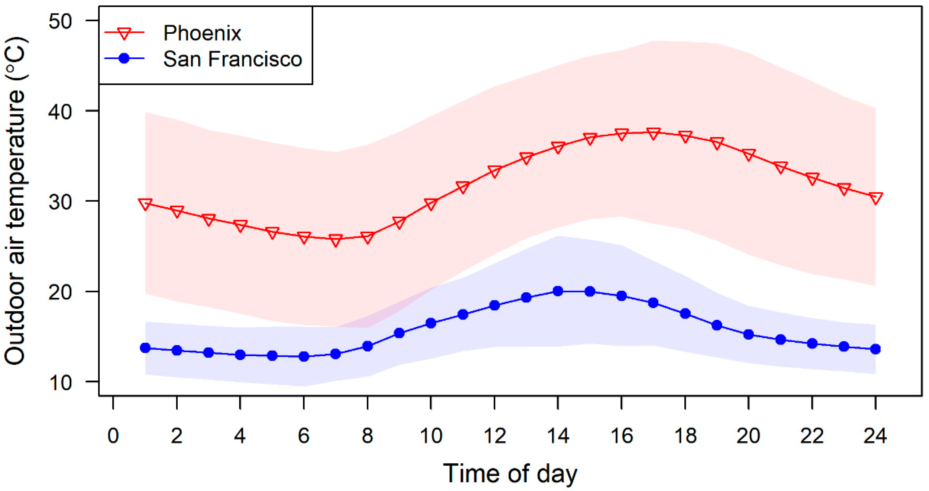
| Location | Phoenix, AZ (climate zone 2B); San Francisco, CA (climate zone 3C) |
| Floor area | 510 m2 |
| No. of floors | 1 |
| Zones | 1 core zone and 4 perimeter zones |
| Aspect ratio | 1.5 |
| Window fraction | 24.4% for South perimeter zone and 19.8% for North, East, and West perimeter zones |
| Cooling system | Air-source heat pump |
| Air distribution | Single-zone constant air volume (CAV) |
| Internal Heat Gains | Intensity (W/m2) | Convective Fraction | Radiant Fraction | Visible Fraction |
|---|---|---|---|---|
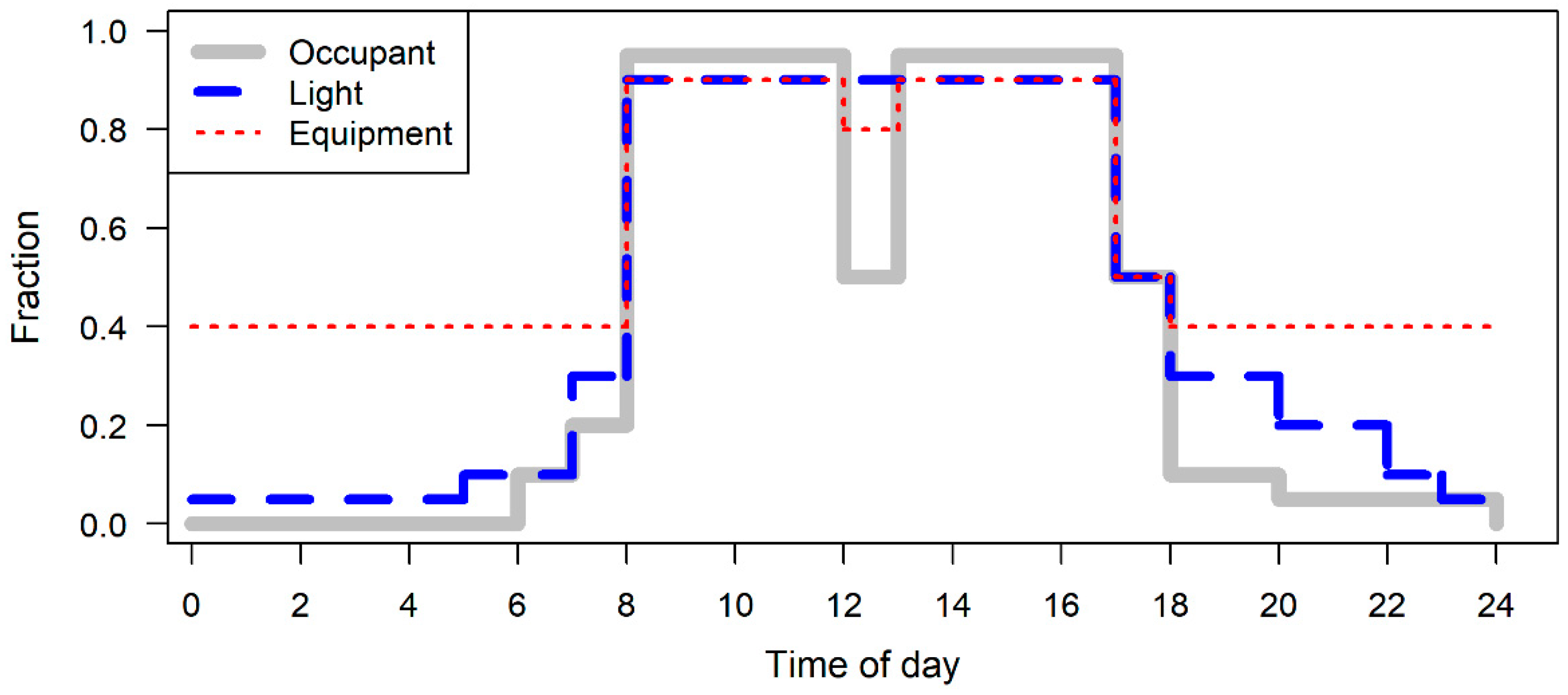
| Occupants | 6.46 (1) | 0.5 | 0.5 | 0 |
| Lights | 10.76 | 0.1 | 0.7 | 0.2 |
| Electric equipment | 10.76 | 0.5 | 0.5 | 0 |
| Case No. | Climate Zone | Cooling Strategy | Floor Configuration | Simulation Duration |
|---|---|---|---|---|
| 1 | Phoenix, AZ (hot and dry) | Base | Bare concrete | 1 June–31 Oct |
| 2 | Concrete + carpet | |||
| 3 | Wood | |||
| 4 | Precooling + GTA | Bare concrete | ||
| 5 | Concrete + carpet | |||
| 6 | Wood | |||
| 7 | San Francisco, CA (warm and marine) | Base | Bare concrete | |
| 8 | Concrete + carpet | |||
| 9 | Wood | |||
| 10 | Precooling + GTA | Bare concrete | ||
| 11 | Concrete + carpet | |||
| 12 | Wood |
| Floor Layer | Conductivity (W/mK) | Density (kg/m3) | Specific Heat (J/kgK) | Thickness (cm) |
|---|---|---|---|---|
| Concrete | 1.311 | 2240 | 836.8 | 10 |
| Wood | 0.12 | 540 | 1210 | 10 |
| Slab insulation | 0.035 | 265 | 1300 | 5 |
| Carpet (synthetic) | 0.060 | 160 | 2500 | 1 |
Publisher’s Note: MDPI stays neutral with regard to jurisdictional claims in published maps and institutional affiliations. |
© 2021 by the authors. Licensee MDPI, Basel, Switzerland. This article is an open access article distributed under the terms and conditions of the Creative Commons Attribution (CC BY) license (https://creativecommons.org/licenses/by/4.0/).
Share and Cite
Ahn, H.; Liu, J.; Kim, D.; Yin, R.; Hong, T.; Piette, M.A. How Can Floor Covering Influence Buildings’ Demand Flexibility? Energies 2021, 14, 3658. https://doi.org/10.3390/en14123658
Ahn H, Liu J, Kim D, Yin R, Hong T, Piette MA. How Can Floor Covering Influence Buildings’ Demand Flexibility? Energies. 2021; 14(12):3658. https://doi.org/10.3390/en14123658
Chicago/Turabian StyleAhn, Hyeunguk, Jingjing Liu, Donghun Kim, Rongxin Yin, Tianzhen Hong, and Mary Ann Piette. 2021. "How Can Floor Covering Influence Buildings’ Demand Flexibility?" Energies 14, no. 12: 3658. https://doi.org/10.3390/en14123658
APA StyleAhn, H., Liu, J., Kim, D., Yin, R., Hong, T., & Piette, M. A. (2021). How Can Floor Covering Influence Buildings’ Demand Flexibility? Energies, 14(12), 3658. https://doi.org/10.3390/en14123658