Flow Characteristics of Preliminary Shutdown and Startup Sequences for a Model Counter-Rotating Pump-Turbine

Abstract

Pumped Hydropower Storage (PHS) is the maturest and most economically viable technology for storing energy and regulating the electrical grid on a large scale. Due to the growing amount of intermittent renewable energy sources, the necessity of maintaining grid stability increases. Most PHS facilities today require a geographical topology with large differences in elevation. The ALPHEUS H2020 EU project has the aim to develop PHS for flat geographical topologies. The present study was concerned with the initial design of a low-head model counter-rotating pump-turbine. The machine was numerically analysed during the shutdown and startup sequences using computational fluid dynamics. The rotational speed of the individual runners was decreased from the design point to stand-still and increased back to the design point, in both pump and turbine modes. As the rotational speeds were close to zero, the flow field was chaotic, and a large flow separation occurred by the blades of the runners. Rapid load variations on the runner blades and reverse flow were encountered in pump mode as the machine lost the ability to produce head. The loads were less severe in the turbine mode sequence. Frequency analyses revealed that the blade passing frequencies and their linear combinations yielded the strongest pulsations in the system.

1. Introduction

The demand to control and regulate the electrical grid to provide grid stability is ever increasing. This is a consequence of the fact that intermittent renewable energy sources, e.g., wind and solar, are on the rise and will continue to increase in the coming decades [1]. Pumped Hydro Storage (PHS) is the maturest and most cost-efficient solution to store energy and thus provide grid stability [2,3,4]. The oldest PHS power plants date back to the late 19th Century [5]. In the year 2019, PHS had a capacity of 158 GW worldwide [3]. Traditionally, PHS facilities require very specific site locations to make them economically feasible. According to Deane et al. [6], the head of the PHS facility is the most essential criterion, and a higher head is preferable. Most research is thus focused on PHS intended for higher heads. The ALPHEUS H2020 EU project (“Augmenting Grid Stability Through Low Head Pumped Hydro Energy Utilization and Storage”) aims to contribute with economically viable PHS solutions for low- to ultra-low-heads [7,8]. The main goals of the ALPHEUS project are to achieve a reversible pump-turbine with a power of 10 MW, a round-trip efficiency of 70–80%, and heads in the region of 2–20 m. The ALPHEUS project focuses on three pump-turbine designs, a shaft-driven Counter-Rotating Pump-Turbine (CRPT), a rim-driven CRPT, and a positive displacement configuration. In the present paper, a model scale of an initial design of the shaft-driven CRPT is considered.

Wintucky and Stewart [9] concluded already in the 1950s that a counter-rotating turbine may have 2–4% higher overall efficiency compared to a single-rotor configuration. The concept of a counter-rotating propeller configuration is commonly associated with marine or aeroplane propulsion systems [10]. In recent years, the counter-rotating propeller configuration has been investigated as a reversible hydropower pump-turbine unit. Furukawa et al. [11] stated in 2007 that a CRPT, compared to a single rotor, can have a smaller shroud diameter, a lower rotational speed, and a wider range of operation at high efficiency with an individual speed control of the two runners. In a multi-objective optimisation of a CRPT, Kim et al. [12] showed that a hydraulic efficiency of close to 80% in turbine mode and above 85% in pump mode could be achieved, for a wide range of operating conditions. A CRPT has been analysed in pump mode with unsteady Computational Fluid Dynamics (CFD) simulations and validated with experimental test data by Momosaki et al. [13]. It was concluded that unsteady computations are required to accurately predict the performance of the CRPT, even at the design point.

Recent studies of Francis-like pump-turbines have shown that it is possible to numerically predict the flow characteristics during transient sequences such as load-rejection and mode-switching [14,15,16,17]. The current study investigated the shutdown and startup sequences for a model-scale CRPT, in both pump and turbine modes. In conventional Francis-like pump-turbines, guide vanes are used to direct and control the flow [18]. In contrast to the various Francis-like pump-turbines, the shaft-driven CPRT in the ALPHEUS project has no guide vanes. It is the head and individual rotational speeds of the runners that determine the point of operation. The transient sequences include a decrease of the runner rotational speeds, from the design point to stand-still. The rotational speeds are later increased from stand-still back to the design point.

2. Design and Operating Conditions

Figure 1 shows the blade geometry of the analysed CRPT, as well as the computational domain. Conventional Francis-like pump-turbines utilise guide vanes to produce angular momentum in turbine mode and to reduce angular momentum in pump mode, thus ensuring high efficiency in both modes. This is not the case for the CRPT as the basic principle of the CRPT is that the upstream runner is designed to have an axial inflow, while the counter-rotating downstream runner makes use of the angular momentum leaving the upstream runner, generating a close to axial flow downstream the runners at the best efficiency point. Figure 1a shows the blade geometries of Runner 1 (red) and Runner 2 (blue). Runner 1 worked as the upstream runner in pump mode and downstream in turbine mode. In this study, the CRPT was at model scale, since the numerical results are later to be validated against experimental test data. Figure 1b shows the full computational domain, the locations of velocity probing lines, and pressure probe P4. The computational domain included the two runners, the hub with support struts, and contraction/expansion sections before/after the machine to focus the kinetic energy. Some parts of the straight pipes were included in the computational domain to keep the boundary conditions at some distance. The total length was 12.8-times the diameter of the runners. In pump mode, the flow was from left to the right, and in turbine mode, it was from right to left.

The blade geometries, shown in Figure 1a, were designed by Advanced Design Technology (ADT) Ltd., as a part of the ALPHEUS H2020 EU project [19]. Runner 1 had eight blades, while Runner 2 consisted of seven blades. The two runners rotated in opposite directions from one another. No guide vanes were utilised, as the upstream runner was designed to have an axial inflow. The runner hub and shroud diameters were 156 mm and 270 mm, respectively. The machine was operated by individually controlling the rotational speed of each runner. At the design point in pump mode, Runner 1 rotated at 1423 rpm and Runner 2 at 1307 rpm. The corresponding rotational speeds in turbine mode were 832 rpm and 749 rpm. The engineering quantities at the design point are summarised in

Table 1. Engineering quantities at the design point in pump and turbine modes.

	Pump	Turbine	Unit
Head	15.3	9.2	m
Power	56.0	20.1	kW
Discharge	333.5	252.9	L/s
Efficiency	89.2	88.2	%

. The net head and power were higher in pump mode since the machine must overcome the hydraulic losses at the test facility. In turbine mode, those losses were subtracted, yielding a lower net head and power. The hydraulic efficiency of the machine was roughly the same in both modes. The head was defined by the total pressure drop of the computational domains of the runners, coloured red and blue in Figure 1b. The efficiency is calculated in pump and turbine modes as:

$$\begin{array}{cc}\hfill {\eta }_{\mathrm{Pump}}=& \frac{\rho gHQ}{P},\hfill \end{array}$$

(1)

$$\begin{array}{cc}\hfill {\eta }_{\mathrm{Turbine}}=& \frac{P}{\rho gHQ}.\hfill \end{array}$$

(2)

Here, $\rho$ is the fluid density, g is the gravity acceleration, H is the head, and P is the power. The power was in this work defined as $P=T_{\mathrm{R}1}{\Omega }_{\mathrm{R}1}+T_{\mathrm{R}2}{\Omega }_{\mathrm{R}2}$, where T is the torque and Ω is the rotational speed in rad/s of the runners. The subscripts R1 and R2 are for Runner 1 and Runner 2, respectively.

3. Methods

The present CRPT was previously evaluated in detail at the design point in both pump and turbine mode, with both steady-state and unsteady numerical simulations [20]. In the present study, shutdown and startup sequences were simulated and analysed using CFD. The numerical simulations were carried out with the OpenFOAM-v1912 open-source CFD software [21,22]. As previously mentioned, the runners rotated at individual speeds. For a given net head, it was the combination of rotational speeds of the runners that controlled the operating point of the machine. Two full shutdown and startup sequences were carried out in the present work, one for each mode. The rotational speeds were first decreased, from the design point to stand-still, and later increased back to the design point. The evaluated transient sequences are shown in Figure 2. The rotational speeds are presented as functions of time for the two modes. At time $t=0$ s, the flow was fully developed at the design point, based on the previous simulations. The shutdown sequences started at time $t_{0,1}=0.2$ $\mathrm{s}$ in both modes. The time from the design point to complete stand-still was 2.6 s and 4.5 s in turbine and pump mode, respectively. The runners were at a stand-still between times $t_{\mathrm{end},1}$ and $t_{0,2}$. The startup sequences started at $t_{0,2}$ and continued to $t_{\mathrm{end},2}$. The entire simulation time was 8.0 s in turbine mode and 11.3 s in pump mode. The transient sequence required less time in turbine mode as the rotational speeds were lower at the design point compared to in pump mode. The rotational speeds were decreased and increased symmetrically by a sinusoidal function as:

$$n_r=\frac{n_{r,\mathrm{DP}}}{2}\left[1+sin\left(\pi \frac{t-t_0}{t_{\mathrm{end}}-t_0}\pm \frac{\pi }{2}\right)\right].$$

(3)

Here, n is the rotational speed in rpm, $n_{\mathrm{DP}}$ is the rotational speed at the design point, t is the time, $t_0$ is the start time of the transient, and $t_{\mathrm{end}}$ is the end time of the transient. Index r is 1 or 2 for the corresponding runner. The ± sign is positive when decreasing the rotational speed and negative when increasing the speed. The sinusoidal shape to change the rotational speed of the runners was chosen since a sinusoidal function allows a smooth transition between two constant rotational speeds.

3.1. Governing Equations and Numerical Schemes

The incompressible Navier–Stokes equations were discretised and solved for a computational mesh using the finite volume method [23,24]. The k-$\omega$ SST-SAS eddy viscosity model was employed to take into account the effects of unresolved turbulence. The SAS modifications to the standard k-$\omega$ SST turbulence model allow for a decrease in the turbulent viscosity where the turbulence may be partially or fully resolved [25]. This turbulence model has recently been successfully used in a number of studies concerning transient operations in a hydropower context [14,15,26]. The simulations were carried out on the full 3D computational domain shown in Figure 1b. Each runner domain rotated individually with a solid body rotation, employing an Arbitrary Mesh Interface (AMI) for the transfer of fluxes at the sliding interfaces [27,28].

The convection terms of the momentum equations were discretised using the second-order accurate Linear-Upwind Stabilised Transport (LUST) scheme [29]. This is a blended scheme, utilising a 75% central differencing scheme (linear), for accuracy, and a 25% second-order upwind scheme (linearUpwind), for stability [30]. The first-order upwind scheme was used to discretise the convection terms in the transport equations for turbulent kinetic energy (k) and specific turbulence dissipation rate ($\omega$). The linear scheme with the Gauss theorem was employed for the gradient schemes of all variables. The implicit, second-order accurate scheme (backward) was used for temporal discretisation. A constant time step of $\Delta t=5\times {10}^{-5}$ $\mathrm{s}$ was used. At the design point, in pump mode, the time step corresponded to a Courant number of less than 2.2 in 90% of the numerical domain, and the average Courant number was less than 0.065. The maximum runner rotation was 0.44° per time step.

The pressure–velocity coupling was handled using the PIMPLE algorithm [30]. The algorithm allows the Courant number to exceed unity by combining the PISO and SIMPLE algorithms. The solver algorithm in the present work was configured with two inner PISO loops and a maximum of ten outer SIMPLE corrector loops. One non-orthogonal corrector step was used within each inner loop. The PIMPLE algorithm interrupts the outer corrector loops if convergence is reached within each time step. The solution was deemed as converged if the absolute tolerance was below ${10}^{-6}$ and ${10}^{-5}$ or the relative tolerance was below $0.1$ and $0.01$, for velocity and pressure, respectively. The absolute tolerance is the solver residual, and the relative tolerance is in relation to the initial solver residual. The solver algorithm always converged within three or four outer corrector loops.

3.2. Boundary Conditions

A total pressure boundary condition was used for the inlet, while a static pressure boundary condition was imposed on the outlet boundary. The flow rate was thus calculated as a part of the solution. A total-to-static pressure difference of 100 kPa and 134 kPa was used in turbine and pump mode, respectively. The total-to-static pressure difference over the computational domain ensured the net head of the CRPT at the design point, presented in Table 1. Note that the net head in the table was defined by the total pressure difference over just the CRPT, and the total-to-static pressure difference concerned the entire computational domain. In OpenFOAM-v1912, the totalPressure boundary condition was used for pressure at both the inlet and the outlet, together with the velocity boundary condition pressureInletOutletVelocity. This combination of boundary conditions has recently been used to accurately simulate a shutdown transient for a high-head Francis model turbine by Uppström et al. [31]. The totalPressure boundary condition corresponds to a static pressure formulation on the boundary as:

$$\begin{array}{cc}\hfill p_{\mathrm{boundary},i}=& p_0-\frac{\rho |{\overrightarrow{u}}_i{|}^2}{2},\mathrm{for}\mathrm{inflow}(\mathrm{at}\mathrm{face}i),\hfill \end{array}$$

(4)

$$\begin{array}{cc}\hfill p_{\mathrm{boundary},i}=& p_0,\mathrm{for}\mathrm{outflow}(\mathrm{at}\mathrm{face}i).\hspace{1em}\hspace{1em}\hspace{1em} \hfill \end{array}$$

(5)

Here, $p_0$ is the user-specified pressure (total for inflow and static for outflow, hence the minus in Equation (4)), $\rho$ is the fluid density, and $\overrightarrow{u}$ is the velocity vector. Index i corresponds to face i on the boundary, meaning that the conditions are applied on a face-by-face basis. The boundary condition imposes a constant total pressure at the inlet faces and constant static pressure at the outlet faces. The pressureInletOutletVelocity boundary condition for the velocity applies a homogeneous Neumann (zero gradient) condition on the outlet faces. At the inlet faces, the velocity is obtained from the internal field in the face normal direction, as described by Fahlbeck [32]. It was essential to use a pressure–velocity boundary condition combination that allows for reverse flow, since the flow direction changes during the shutdown and startup operations in pump mode.

3.3. Computational Mesh

The computational mesh was divided into four regions, one for each runner and one for each of the contraction/expansion regions upstream and downstream the runners. The meshes of the runners were mostly block-structured, whereas the contraction/expansion regions consisted of 6 layers of prism boundary layer cells near the walls and unstructured tetrahedral core cells, as shown in Figure 3. The shroud tip clearance was 0.67 mm, and 8 layers of hexahedral and triangular prism cells were used in the tip clearance region. The mesh was finest at the runners, and gradually coarser further away from the runners. The surface mesh of one blade passage for the two runners is shown in Figure 3a, and the refined mesh regions close to the runners are shown in Figure 3b.

Table 2. Mesh details.

Region	Cells × 106	${\mathit{y}}_{\mathbf{90}\mathbf{\%}}^{\mathbf{+}}$
Runner 1	1.90	45
Runner 2	1.97	54
Upstream/downstream	2 × 1.94	46
Full domain	7.75	50

presents a summary of the meshes for different regions. Note that the upstream and downstream regions utilised the same mesh. The total number of cells was 7.75 million, and the different regions contained roughly the same number of cells. The $y_{90\%}^{+}$ values in Table 2 denote the maximum $y^{+}$ values in 90% of the region. They were obtained in pump mode at a time step before the transient operations had commenced. The $y^{+}$ value was less than 50 in 90% of the computational domain. Wall functions that adapted to all $y+$ values were used. In OpenFOAM-v1912, the wall boundary conditions kqRWallFunction for turbulent kinetic energy (k), omegaWallFunction for specific dissipation rate ($\omega$) and nutkWallFunction for turbulent viscosity were applied.

4. Results and Discussion

The outcome of the numerical simulations is presented and discussed in this section. The section is divided into two sub-sections, where first, the analysis in turbine mode is discussed, followed by the pump mode investigation. Recall the time and rotational speeds shown in Figure 2, as both are referred to in this section.

4.1. Turbine Mode Transient Sequence

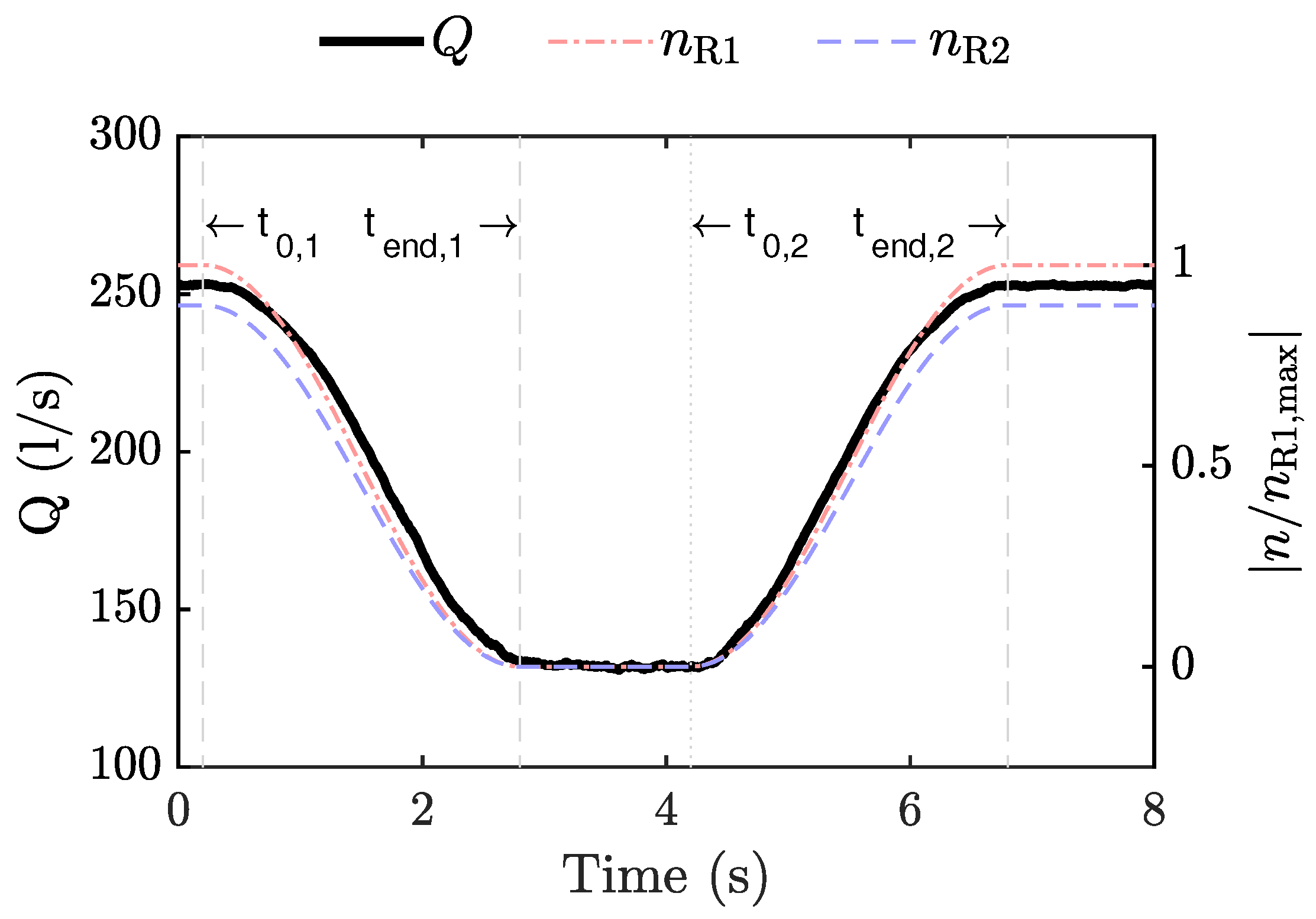
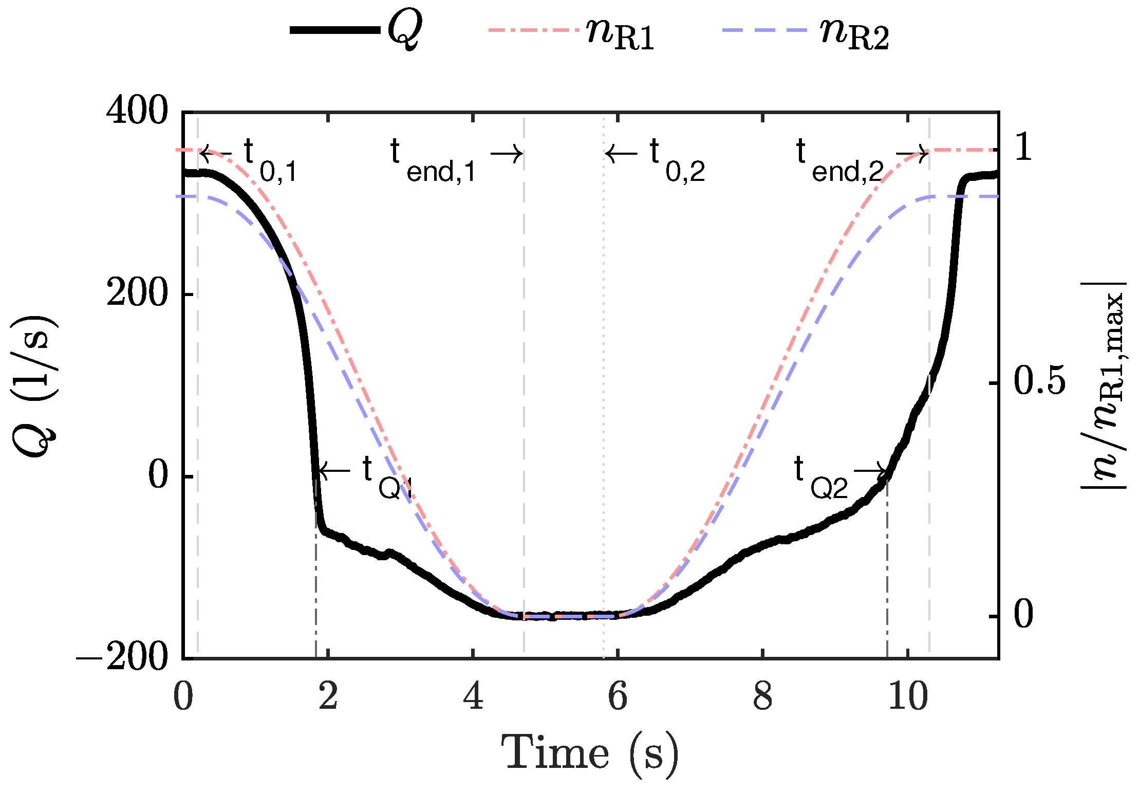
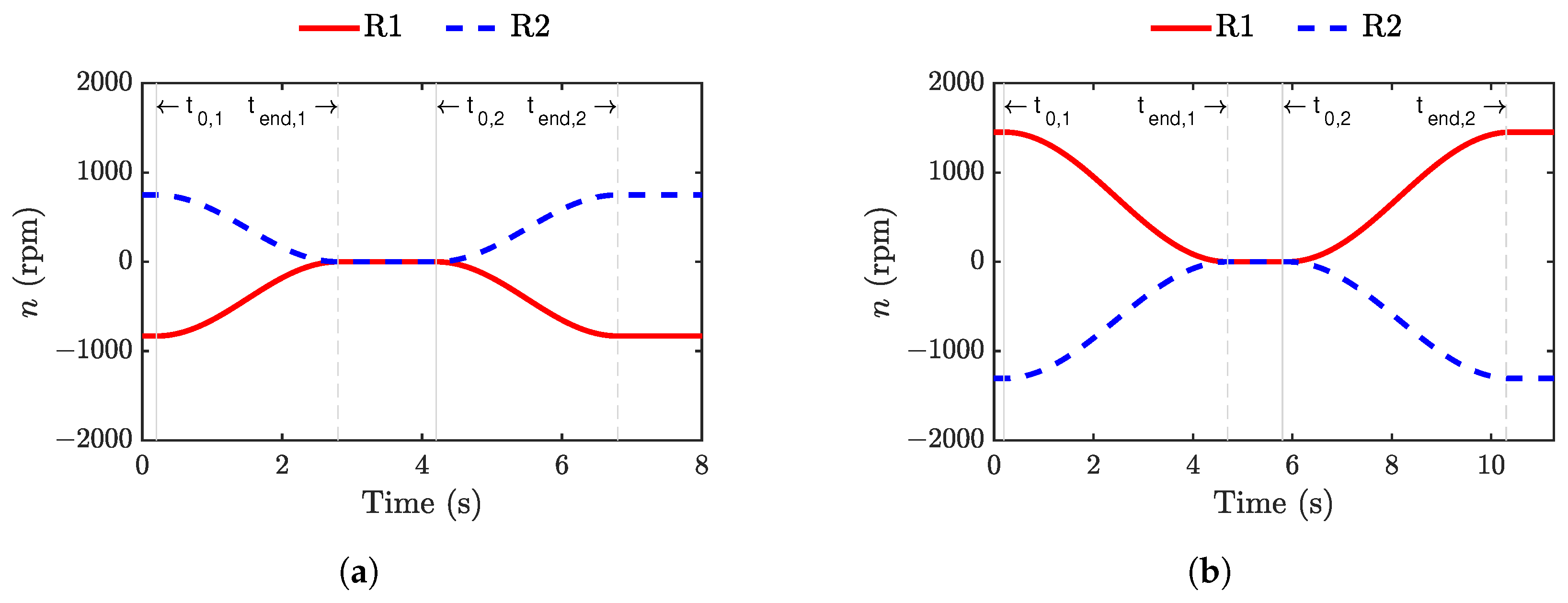
The shutdown and startup sequences in turbine mode are analysed here. The numerically predicted flow rate is shown in Figure 4 as a function of time. The flow rate was initially 253 L/s, at the design point. The rotational speed of the runners started to decrease at $t_{0,1}$, and the flow rate followed the decreasing rotational speed. This was because with a lower rotational speed, the CRPT was not effectively extracting energy from the flow, and the losses that reduced the flow rate were increasing. As the runners were at a stand-still ($t_{\mathrm{end},1}<t<t_{0,2}$), the machine was simply a large obstacle in the flow path, and the flow rate was 132 L/s. This was almost half the flow rate of the design point. At $t_{0,2}$, the runner rotational speeds started to increase, and the flow rate increased accordingly. The change of flow rate occurred symmetrically in the turbine mode sequences with the change of the rotational speeds. This was not the case in pump mode, as discussed later.

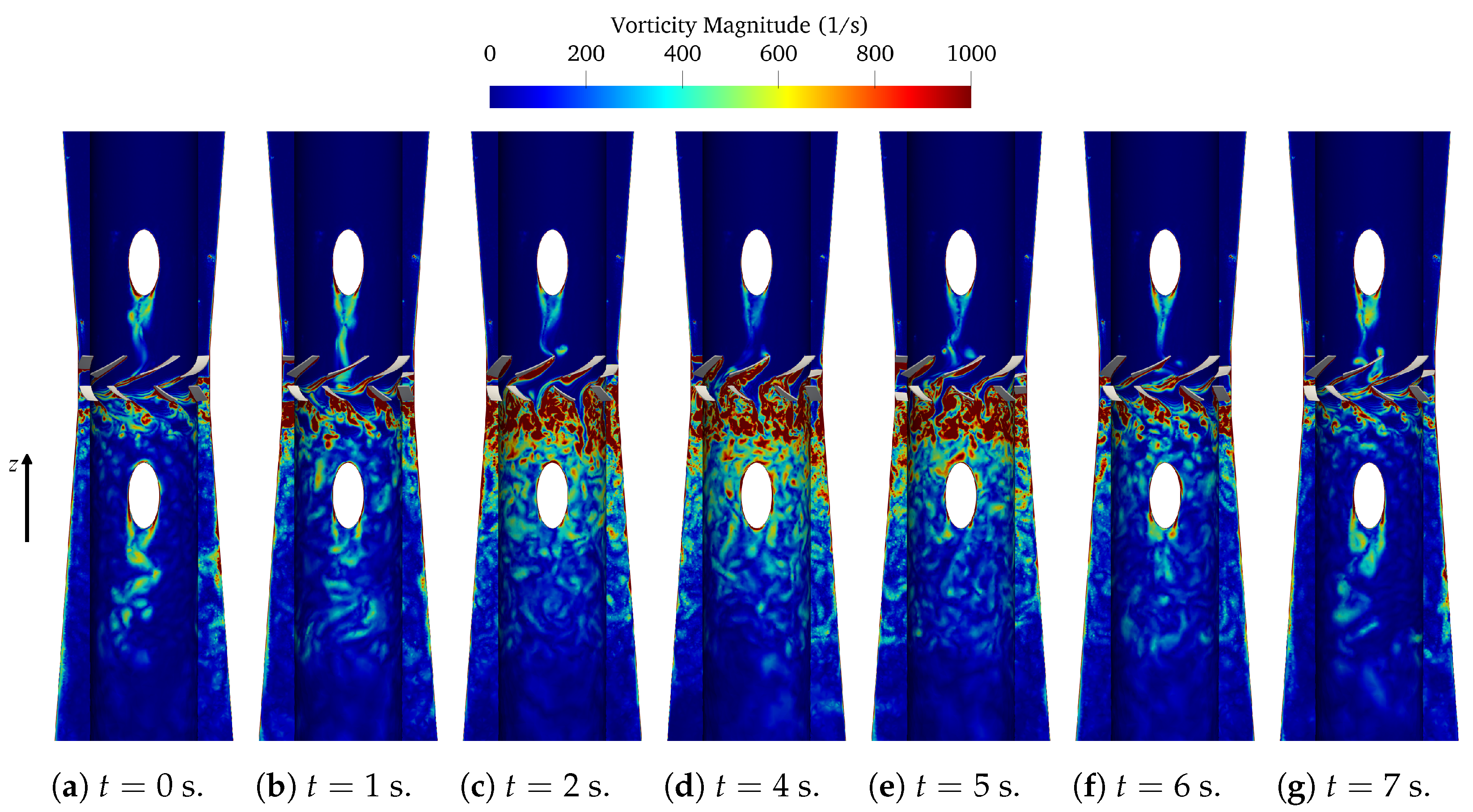
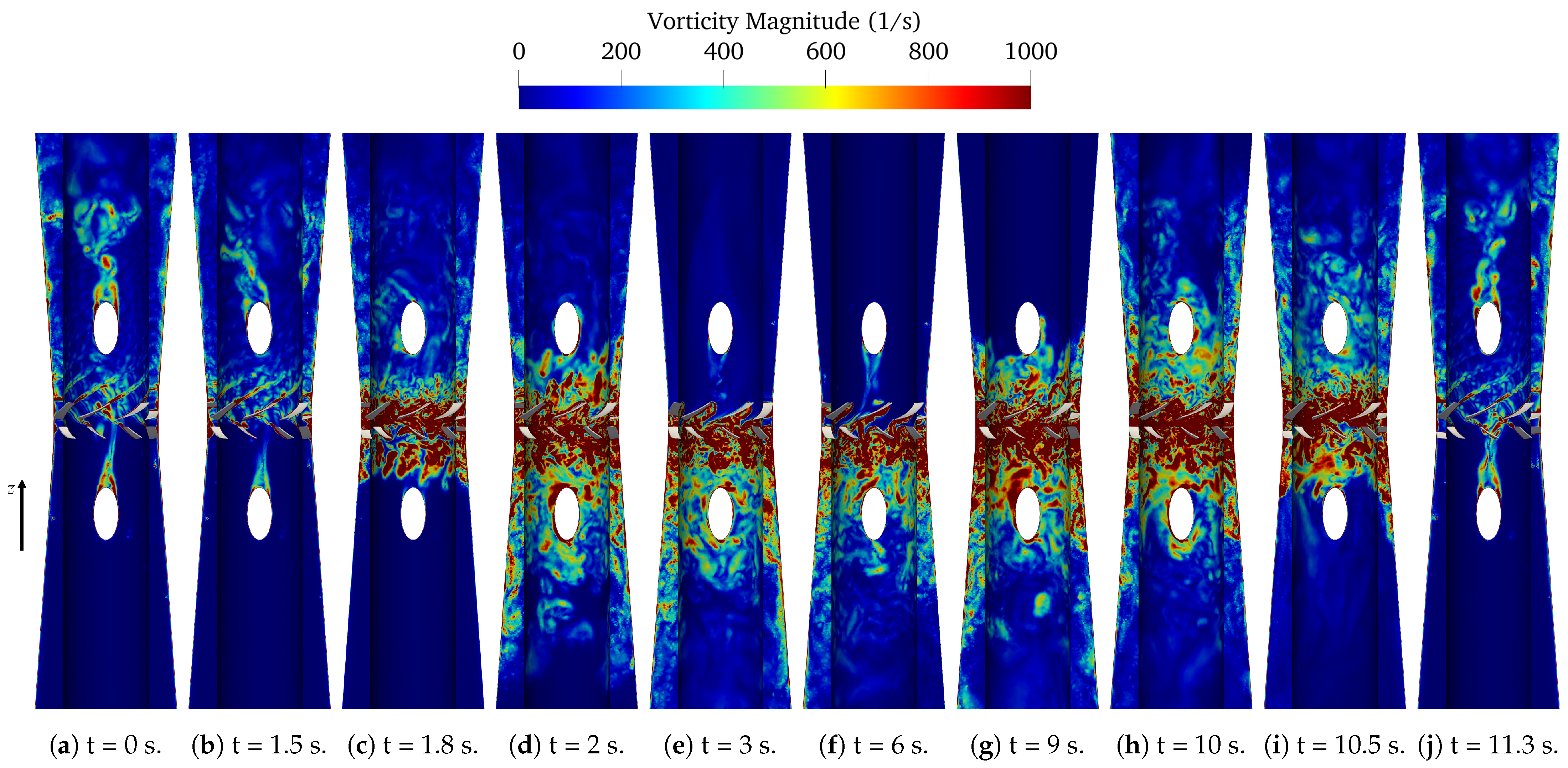
With a decreasing rotational speed, unfavourable flow structures increased in scale and number, and the flow became massively separated after the CRPT, as shown by the vorticity magnitude in Figure 5. Note that the flow was from top to bottom, and that vorticity is defined as the curl of the velocity. At $t=0$ s (Figure 5a), the flow was rather axial, both before and after the runners, and the vortex shedding of the downstream support-strut was captured. As the rotational speeds decreased, it can be seen in Figure 5a–d that the flow at the blades of Runner 1 (lower one) first started to separate, then the same happened also at Runner 2. The reduction in rotational speed of Runner 2 increased the swirl coming to Runner 1. At the same time, Runner 1 was also decreasing its rotational speed, which further deteriorated the relative flow angle at the leading edges of Runner 1’s blades. This is why the flow behind Runner 1 separated much more than that of Runner 2. This suggests that Runner 1 should maintain its rotational speed in the initial phase, but at some point, it must reduce its speed to stand-still and thus go through such unfavourable conditions. However, at that point, there would also be a valve that closed and further reduced the flow rate of the machine. Suggesting the optimum shutdown and startup sequences to minimise the damaging effects of the large flow separation structures remains to be investigated. At time $t=4$ s, the runners were both at a stand-still, and a chaotic flow field had developed downstream the runners. This was mainly generated by a massive separation on Runner 1’s blades, although also, the separation on Runner 2’s blades increased significantly. As the rotational speed of the runners increased, the efficient tandem operation of the two runners became apparent again. This is shown by Figure 5d–g, as the unfavourable flow structures diminished during the startup sequence. As for the flow rate variation, shown in Figure 4, the variation in unfavourable flow structures (and thus losses) was very similar for the shutdown and startup sequences. However, the vortex shedding behind the downstream support-strut needed some additional time to develop after $t=7$ s.

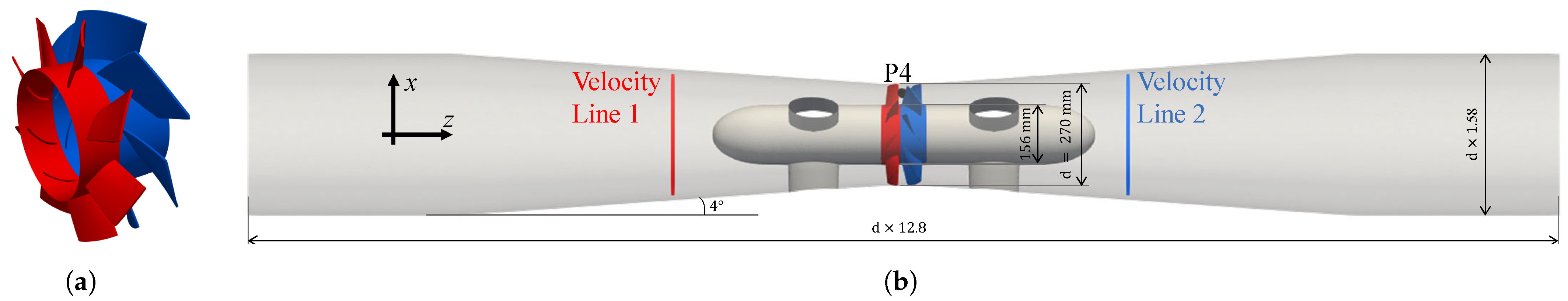
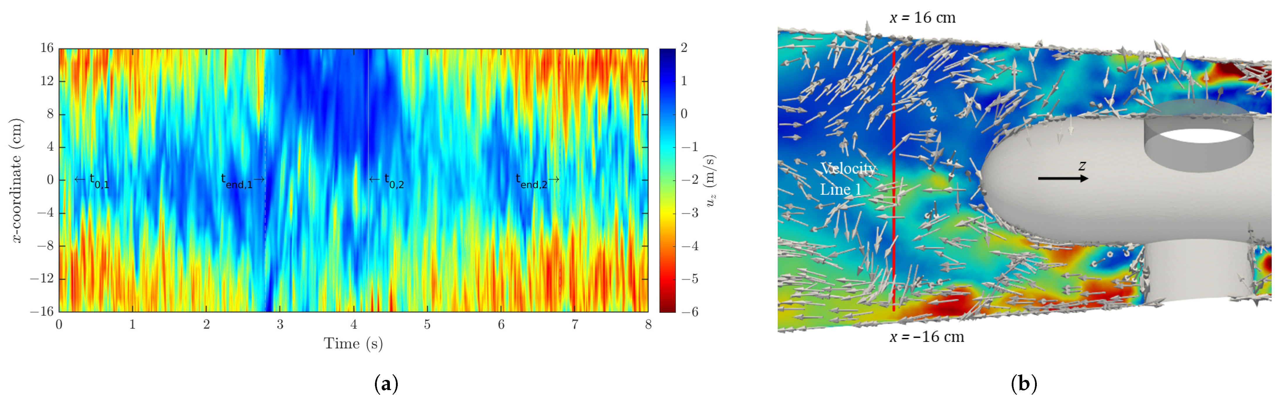
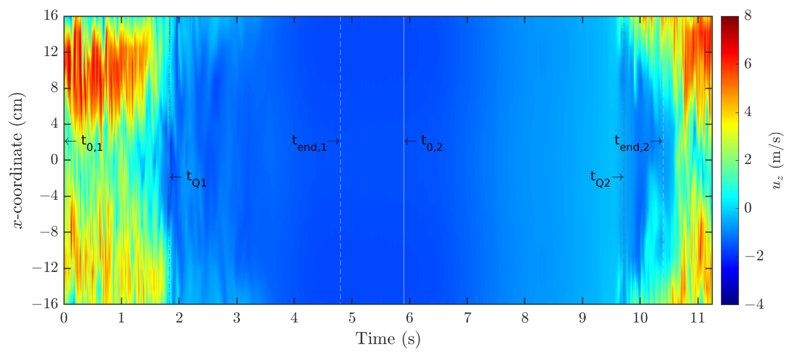
The axial velocity at probing Line 1 (see the location in Figure 1b) is shown in Figure 6a as a contour over the x-coordinate and time. The flow profile was rather similar over the centreline at the earlier and later time steps, where the machine was working at the design point condition. There was not a distinct difference in the largest magnitude of the axial velocity at $t<1$ and $t>7$ s, for positive and negative x-coordinates. This was despite the fact that a support-strut was located between the runners and the line for negative x-coordinates. This means that the flow was not purely axial downstream the runners and that there was some swirl leaving the runners. The remaining swirl rotated the flow profile, causing a close to symmetric flow profile at the velocity line. As the runners were at a stand-still ($t_{\mathrm{end},1}<t<t_{0,2}$), the flow profile was far from symmetric. At $x>0$ cm, close to zero and reverse flow were encountered at the velocity line. This was explained by the velocity vectors shown in Figure 6b. At the position of Line 1 (red), the flow rotated back towards the runners. This was while the flow was in the correct direction at the negative x-coordinates. The reason for the flow appearance at the velocity line was connected to the location of Line 1 in relation to the stand-still position of the runner blades. When the runners were at a stand-still, wakes downstream the runners developed depending on how the runners were oriented. In general, the flow was rather chaotic downstream the runners as the rotational speeds were small or zero. This was because the flow was massively separated at this point, and the resolved solution was expected to show randomness as the SAS model resolved part of the turbulent spectrum. The solver residuals were at this stage in the order of ${10}^{-6}$ for momentum, ${10}^{-5}$ for pressure, and ${10}^{-10}$ for continuity, which indicated a relatively small error at each time step.

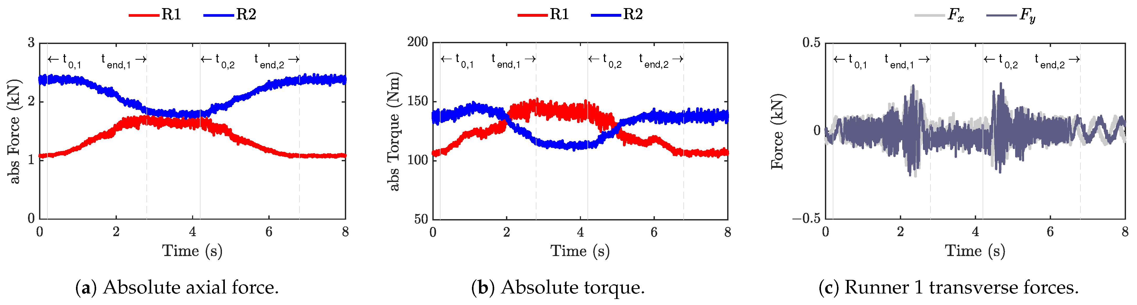
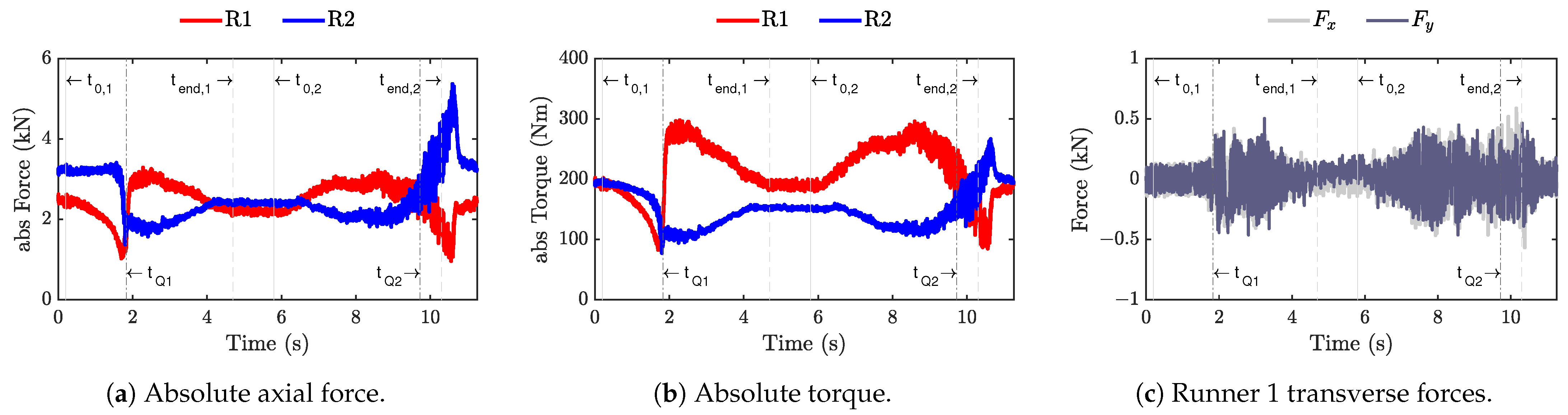
Figure 7a,b shows the absolute axial force and absolute torque, respectively, during the turbine mode transients. The forces and torque acting on the runners were from integrated normal and shear stresses on the hub and blade surfaces of the runners. In the discussions below, the word absolute is dropped for brevity. The axial force and torque showed a smooth variation without any drastic peaks. As the rotational speeds decreased, the loads of Runner 1 increased and the loads of Runner 2 decreased. The axial force and torque was to a large extent a function of the head, or total pressure drop between the two reservoirs. In this study, the reservoirs were represented by the pressure boundary conditions at the inlet and the outlet. Thus, the summation of the loads of the two runners must always be rather constant in turbine mode. As the flow of Runner 1 started to separate, due to the intensified swirl coming from Runner 2, the loads increased for Runner 1. As a consequence of the load increase for Runner 1, Runner 2 experienced a decrease in loads. The axial force on the upstream runner was slightly higher when the runners were at a stand-still. This was because Runner 2 faced the upper reservoir, and Runner 1 was in the wake of Runner 2. The torque was higher for Runner 1 since Runner 2 directed the flow in an unfavourable direction towards Runner 1 at a stand-still. When the startup sequence was initiated, at $t_{0,2}$, the upstream runner experienced an axial load increase while the downstream runner experienced a load decrease. The torque followed the trends of the axial force during the transient sequences. The force variation in the transverse directions for Runner 1 is shown in Figure 7c as a function of time during the transient sequences in turbine mode. The transverse force fluctuations were rather calm until the rotational speed was low. Between $t=2$ s to $t_{\mathrm{end},1}$ and $t=5$ s to $t_{0,2}$, large transverse force fluctuations were detected for Runner 1. They most likely arose from the flow separation at the blades of Runner 1, shown in Figure 5. The flow separation caused the formation of large chaotic flow structures at Runner 1’s blades. This generated large force fluctuations in the transverse directions. The transverse forces for Runner 2 (not shown here) did not show such fluctuations when close to stand-still, since Runner 2 did not experience such massive flow separation as Runner 1.

Short-Time Fourier Transform (STFT) was performed to analyse the quantities in the frequency domain, due to the time-varying nature of the obtained signals. Frequency analysis was carried out on the fluctuating component of the pressure-probe P4, shown in Figure 1b, and the forces acting on the runner surfaces. The fluctuating component of a signal was calculated as:

$${\phi }^{\prime }=\phi -\overline{\phi }.$$

(6)

Here, $\phi$ is the signal of an arbitrary quantity and $\overline{\phi }$ is the instantaneous average of the signal. The instantaneous average was calculated with the Savitzky–Golay filter [33]. STFT is similar to performing a Fast Fourier Transform (FFT) in different time spans. The STFT uses a window averaging and the FFT average over the whole signal [34]. The window size should be chosen in a way to capture all the physical fluctuations. Here, a window size of 0.1 s was chosen to resolve all the high- and low-frequency oscillations. The frequency analysis was performed using the signal processing toolbox of MATLAB and visualised through a spectrogram. Pressure probe P4, located between the runners, was subjected to an STFT analysis in the turbine mode sequences. 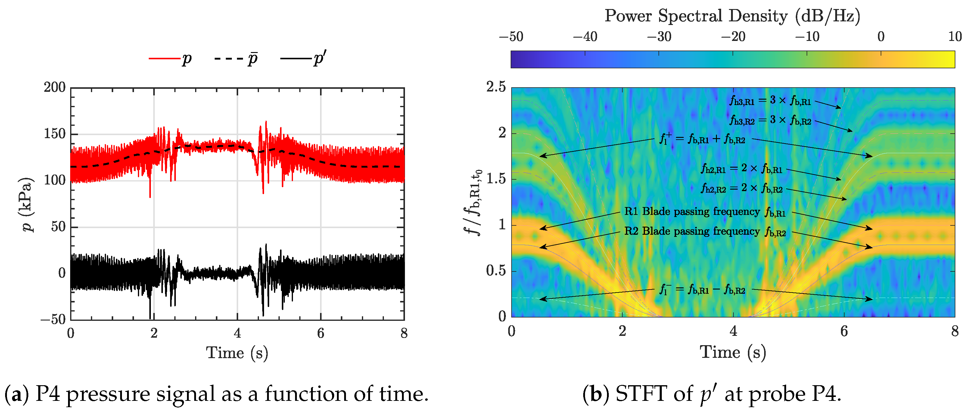The fluctuating part of the pressure signal was obtained according to Equation (6). The static, average, and fluctuating pressures at P4 are shown in Figure 8a. It was evident from the pressure signal, p, that the instantaneous average, $\overline{p}$, was required in order to calculate the true fluctuating component, $p^{\prime }$. This was because the pressure signal did not fluctuate around a fixed value as the rotational speeds were changed. Figure 8b shows an STFT, in a spectrogram, of the fluctuating part of the pressure at P4. The blade passing frequencies, $f_{\mathrm{b},\mathrm{R}1}$ and $f_{\mathrm{b},\mathrm{R}2}$, of the runners showed the highest power in the frequency domain. The second harmonic of the blade passing frequencies, $f_{\mathrm{h}2}$, were also apparent for both runners, but evidently not as powerful as the main frequencies. The third harmonic, $f_{\mathrm{h}3}$, was seen at an even weaker power than the second harmonic. Linear combinations of the blade passing frequencies, $f_{\mathrm{l}}$, were also recognised through the transient. In a turbomachinery application, it is expected that the blade passing frequency is the dominating frequency close to the runners. This is because the runners produces and cuts strong wakes, resulting in pressure pulsations. The closer one is to the runners, the stronger the dynamics of the runners. The linear combination, $f_{\mathrm{l}}^{-}$ and $f_{\mathrm{l}}^{+}$, of the blade passing frequencies were caused by runner–runner interaction, as the downstream runner cut the wakes of the upstream runner. Between the times $t\approx 2$ s and $t\approx 5$ s, a wider range of white noise was seen in the frequency domain. This was caused by the massive flow separation at the blades of runners, shown in Figure 5c–e. The white noise showed a peak in power at the same times as the oscillations for the transverse forces for Runner 1 increased (Figure 7c). The unfavourable oscillations noted as the rotational speed was small should be further analysed and minimised to increase the lifetime of the machine.

4.2. Pump Mode Transient Sequence

In pump mode, the machine must produce sufficient head to overcome the height elevation and the hydraulic losses between the upper and lower reservoir. If the machine cannot produce enough head, the flow will change direction, and the CRPT no longer works as a pump, but as a mixer. During transient sequences in pump mode, the rotational speed of the runners changed according to Figure 2b. At the initial time step, the machine operated at the design point with a flow rate of 334 L/s and a net head of 15 m. Figure 9 shows how the flow rate varied as a function of time during the transient sequences in pump mode. The flow rate was here defined as positive in the preferred pump mode direction (positive z-direction) and negative as the flow was in reversed direction. The flow rate decelerated with the decreasing rotational speed of the runners. At $t_{\mathrm{Q}1}$, roughly one third into the shutdown sequence, the pump lost the ability to produce enough head. After $t_{\mathrm{Q}1}$, the flow accelerated in the reverse direction (identified here by a negative flow rate value). The rotational speeds of the runners were at this time 1031 rpm and $-928$ rpm for Runners 1 and 2, respectively. As the runners were at a stand-still, $t_{\mathrm{end},1}<t<t_{0,2}$, the flow rate was 153 L/s in the reverse direction. When increasing the rotational speeds, $t>t_{0,2}$, it was evident that there were hysteresis effects in the flow. Between $t_{0,2}$ and $t\approx 6.5$ s, the flow rate slowly decelerated. As the rotational speeds increased further, the machine started to build up some pressure. At $t>9$ $\mathrm{s}$, the flow rate was rapidly decelerated up to $t_{\mathrm{Q}2}=9.72$ s. At this point, the head of the machine balanced the head of the system as the flow rate was zero. The flow rate started to accelerate rapidly after $t_{\mathrm{Q}2}$. Observe that the flow rate continued to accelerate after $t_{\mathrm{end},2}$, despite the fact that the runners had a constant speed after this point. This showed that it was not only the rotational speed of the runners that determined the flow rate. This was because it took time for the flow to adjust to the rotational speed, and it depended on if the flow was accelerated or decelerated to the point of operation.

Flow structures during the transient sequences in pump mode are visualised in Figure 10 with the vorticity magnitude at a number of time steps. The preferred flow direction was from bottom to top, when the machine was functioning properly as a pump. The flow structures changed drastically in number and scale during the shutdown and startup sequences. At time $t=0$ $\mathrm{s}$, the CRPT operated at the design point. No large structures were apparent as the machine managed to maintain a close to axial flow downstream the runners. Vortex shedding from the support-struts was clearly visible at this stage. Already at $t=1.5$ s, the machine was less efficient as a pump. This is shown in Figure 10b by the large angle of the vortices of the downstream support-strut. Between $t=1.5$ and 2 s, the flow changed direction, and the machine was no longer able to pump the water in the preferred direction. At the intermediate time step, $t=1.8$ s, the machine struggled to balance the flow, and large separation occurred by the blades of both runners. As time progressed (Figure 10d,e), the rotational speeds decreased further, and the large flow structures followed the reverse flow direction. At time $t=6$ s, the runners were almost at a stand-still. The turbulent flow field was at this stage fully developed in the reverse flow direction, as shown in Figure 10f. The flow field was heavily separated by the blades of the runners at the stand-still position. The rotational speed now increased, and at $t=9$ s, the runners struggled to build up sufficient head and force the flow in the correct pump mode direction. This is shown by the large flow structures on both sides of the runners in Figure 10g,h. By time $t=10.5$ s, the machine pushed the flow in the preferred direction. This is shown in Figure 10g, as the flow structures now started to travel downstream the runners in the preferred direction. At the final time step, $t=11.3$ s, most of the flow structures were flushed out of the domain, and the machine operated at the design point.

Figure 11 shows the axial velocity during the shutdown and startup sequences at Velocity Line 2 in pump mode. Velocity Line 2 is defined in Figure 1b, and it was located downstream the runners when the machine acted as a pump. Before the reverse flow was encountered, $t<t_{\mathrm{Q}1}$, the peak axial velocity was found at a vertical position of $x\approx 10$ cm. A similar, but smaller, peak was noted at $x\approx -10$ cm. The axial velocity was less at the negative x-coordinate due to the position of a support-strut in relation to Velocity Line 2. The axial velocity decelerated and accelerated quickly as the flow changed direction. The flow had a rather flat profile between $t\approx 3$ and 8 s. The velocity rapidly changed at $t\gtrsim 9$ s as the pump built up the head and pushed the flow in the correct direction. At the final time steps, $t>10.5$ s, the familiar pattern from the initial time steps was present.

Figure 12a,b show the absolute axial force and absolute torque as a function of time during the pump mode transients. In the following discussion, the word absolute is dropped, for brevity. The axial load on Runner 1, initially upstream, decreased with the rotational speed before the flow direction reversed. At the same time, the axial force on Runner 2, initially downstream, was rather constant. At the time of zero flow rate, $t_{\mathrm{Q}1}$, a sudden decrease in both axial force and torque was encountered for Runner 2. As a consequence of this, Runner 1 had a rapid load increase. This means that Runner 2 stopped functioning as a pump before Runner 1 and that Runner 1 had to work against the head of the upper reservoir on its own to a larger extent. As the pressure drop over Runner 2 decreased, the loads on the runner followed. This produced a larger pressure drop, and loads, for Runner 1 as it struggled to produce sufficient head. As the rotational speeds continued to decrease, the axial load became similar for the runners. When the runners were at a stand-still, Runner 2 exhibited a slightly larger axial force than Runner 1. This was because Runner 2 was now upstream and facing the upper reservoir. Runner 1 was now downstream and located in the wakes of Runner 2. As the rotational speeds started to increase, the loads on Runner 1 followed, while the loads on Runner 2 decreased. When approaching the change in flow direction, $t_{\mathrm{Q}2}$, the reverse phenomena was noted, and at $t_{\mathrm{Q}2}$, the axial forces of the runners matched one another. After this point, Runner 1 experienced a large decrease in axial force and torque, and Runner 2 had a rapid increase, until the tipping-point at $t\approx 10.6$ s was reached. A plausible explanation for the load decrease for Runner 1 and the load increase for Runner 2 is as follows. Runner 2 managed to build up head before Runner 1, which means a large pressure drop and thus loads for Runner 2. This was because Runner 1 did not yet manage to produce sufficient pressure just upstream of Runner 2. After the tipping-point, the axial force and torque converged to their initial values. The rapid variations of the axial force and torque were most likely not a desirable feature, as large loads can damage or deteriorate the machine prematurely. By examining the forces in the transverse directions for Runner 1, shown in Figure 12c, large oscillations were noted between $t_{\mathrm{Q}1}$ and $t_{\mathrm{Q}2}$. These force variations in the transverse direction most likely arose from the chaotic flow separation occurring by the blades of the runners. The transverse force fluctuations may have a negative impact on the lifetime of the machine. This is because large fluctuating forces are well connected to fatigue.

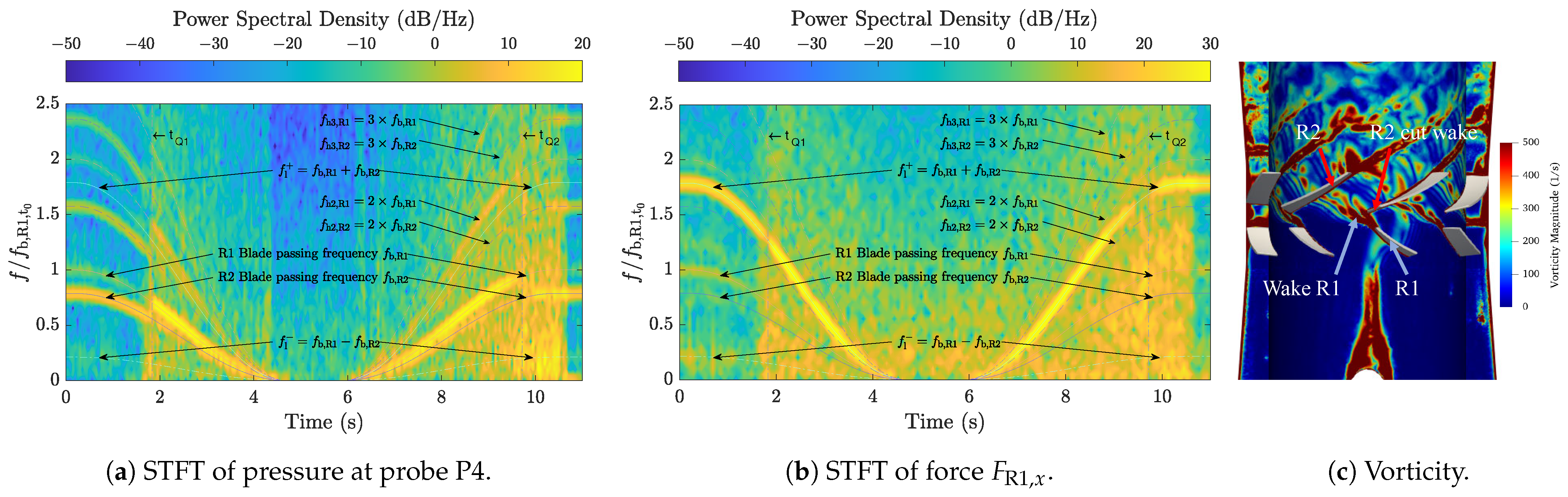
In Figure 13a,b, the STFT for pressure probe P4 and the transverse force $F_{\mathrm{R}1,x}$ are presented. P4 was located between the runners, and $F_{\mathrm{R}1,x}$ was the force in the x-direction on Runner 1. At the pressure probe P4, the blade passing frequencies of the runners, $f_{\mathrm{b},\mathrm{R}1}$ and $f_{\mathrm{b},\mathrm{R}2}$, showed a strong power through the transient sequences. At the initial and final time steps ($t_{\mathrm{Q}1}>t>t_{\mathrm{Q}2}$), the blade passing frequency of Runner 2, $f_{\mathrm{b},\mathrm{R}2}$, showed a stronger power than the blade passing frequency of Runner 1, $f_{\mathrm{b},\mathrm{R}1}$. As the flow rate changed direction ($t=t_{\mathrm{Q}1}$), $f_{\mathrm{b},\mathrm{R}1}$ exceeded $f_{\mathrm{b},\mathrm{R}2}$ in intensity. The Runner 1 blade passing frequency was in fact stronger than that of Runner 2 until the flow was once again reversed to the preferred direction ($t=t_{\mathrm{Q}2}$). Hence, it was found that the stagnation pressure of the downstream runner was always stronger than the wakes from the upstream runner at P4. This was because Runner 1 was initially upstream and Runner 2 downstream, so as the flow changed direction, the strongest blade passing frequency changed as well. The second harmonic frequencies of Runner 2, $f_{\mathrm{h}2,\mathrm{R}2}$, and Runner 1, $f_{\mathrm{h}2,\mathrm{R}1}$, showed the same behaviour as the main blade passing frequencies. The third harmonic frequencies, $f_{\mathrm{h}3}$, and linear combinations, $f_l^{+}$ and $f_l^{-}$, of the blade passing frequencies were apparent at P4, but at a lower intensity. For the transverse force $F_{\mathrm{R}1,x}$ (Figure 13b), the positive linear combination of the blade passing frequencies, $f_l^{+}$, of the runners showed the strongest power throughout the transients. The blade passing frequencies, $f_{\mathrm{b},\mathrm{R}1}$ and $f_{\mathrm{b},\mathrm{R}2}$, of the two runners were also clearly visible for $F_{\mathrm{R}1,x}$, but not as strong as the positive linear combination. An explanation why it was the positive linear combination that had a decisive impact is as follows. The pulsations from each runner were caused by the wakes of each runner, and the linear combination, on the other hand, was caused by the cutting of the upstream runner wakes by the downstream runner. This phenomenon is shown at the design point in Figure 13c. Here, Runner 2 was downstream, and it cut the wakes of the upstream Runner 1. The wakes from the upstream runner were a low-pressure zone. It was cut by a high, stagnation, pressure from the leading edge of the downstream runner. This interaction impacted the pressure, and thus force, pulsations on the runners. The large pressure difference explained why the positive linear combination of the blade passing frequency had a strong impact on the transverse force component, $F_{\mathrm{R}1,x}$. As stated by Lengani et al. [35], any linear combination of the blade passing frequencies can possibly be excited due to the runner–runner interaction of a counter-rotating machine. In addition to the positive linear combination, $f_l^{+}$, the negative linear combination, $f_l^{-}$, was also seen through the transient sequences. At the pressure probe (Figure 13a), the signal showed a significant amount of noise at the times related to a zero flow rate. This was because flow structures were formed and dissolved irregularly over a wide range of scales between the runners, as indicated by the vorticity in Figure 10. The pressure signal was rather smooth as the runners were at a stand-still. The STFT for the transverse force, shown in Figure 13b, revealed a wider range of frequencies and white noise in the signal. This was plausibly due to the flow separation occurring by the blades of the runner. The flow separation interacted with the transverse force over a wide range of scales, which explained the white noise. It was however the typical frequencies correlated to the rotation of the runners that had the strongest power.

5. Conclusions

In this study, preliminary shutdown and startup sequences were numerically evaluated for a model counter-rotating pump-turbine in both pump and turbine modes. The rotational speed of each runner decreased from the design point to a stand-still, and increased back to the design point. As the rotational speed was close to zero, the flow field was highly unstable, and large flow structures were encountered. In turbine mode, the flow rate changed symmetrically with the rotational speed of the runners. In pump mode, reverse flow was captured as the machine lost the ability to build up sufficient head. Hysteresis effects in the flow field were evident in the startup sequence in pump mode. This was because it took time for the flow to accelerate due to the changes in the rotational speed of the runners.

The rapid load variations that occur in low- or reversed flow conditions may lead to fatigue or damage the machine prematurely. The largest load variations occurred in pump mode, while they were less substantial in turbine mode. The shutdown and startup sequences need to be optimised in pump mode to minimise the loads on the runners. A valve should be added to reduce the flow rate to zero as the machine is stopped, and the operation of the valve should also be part of the optimisation procedure.

The main observed frequencies were related to the runners’ blade passing frequencies. The strongest pulsations for a pressure probe located between the runners were in both pump and turbine mode, mostly correlated directly to the blade passing frequencies. In pump mode, it was found that the blade passing frequency of the downstream runner had a stronger power than the upstream runner. The positive linear combination of the blade passing frequencies showed the highest power for a transverse force component in pump mode. The harmonics of the main frequencies were also clearly visible through the transient sequences. A wide range of stochastic frequencies were excited as flow separation occurred by the blades of the runners, in both modes.

This study ultimately demonstrated that it is crucial to investigate transient sequences for the counter-rotating pump-turbine. One of the main reasons to use pumped hydro storage is to provide grid stability. To enable this in an effective manner, the knowledge of modelling and predicting the transient operations of the machine is of uttermost importance to ensure a high and stable production of renewable energy. The numerical framework presented in study demonstrated its functionality to predict and simulate transient shutdown and startup sequences for a novel counter-rotating pump-turbine. The suggested simulation strategy managed to capture some of the essential and expected flow phenomena, such as: vortex-shedding, flow separation, reversing the flow direction in pump mode, frequencies correlated with the runners, etc. It was hence concluded that the suggested numerical framework can be used to study the counter-rotating pump-turbine in time varying load conditions and transient sequences.

References

1. IEA. Renewables 2020; IEA: Paris, France, 2020; Available online: https://www.iea.org/reports/renewables-2020 (accessed on 6 June 2021).
2. IEA. Will Pumped Storage Hydropower Expand More Quickly Than Stationary Battery Storage? IEA: Paris, France, 2019; Available online: https://www.iea.org/articles/will-pumped-storage-hydropower-expand-more-quickly-than-stationary-battery-storage (accessed on 6 June 2021).
3. IHA. 2020 Hydropower Status; IHA Central Office: London, UK, 2020. [Google Scholar]
4. Luo, X.; Wang, J.; Dooner, M.; Clarke, J. Overview of current development in electrical energy storage technologies and the application potential in power system operation. Appl. Energy 2015, 137. [Google Scholar] [CrossRef] [Green Version]
5. Rehman, S.; Al-Hadhrami, L.M.; Alam, M.M. Pumped hydro energy storage system: A technological review. Renew. Sustain. Energy Rev. 2015, 44. [Google Scholar] [CrossRef]
6. Deane, J.P.; Ó Gallachóir, B.P.; McKeogh, E.J. Techno-economic review of existing and new pumped hydro energy storage plant. Renew. Sustain. Energy Rev. 2010, 14, 1293–1302. [Google Scholar] [CrossRef]
7. ALPHEUS H2020. Available online: https://alpheus-h2020.eu/ (accessed on 26 April 2021).
8. Qudaih, M.; Engel, B.; Truijen, D.; Kooning, J.; Stockman, K.; Hoffstaedt, J.; Jarquin Laguna, A.; Ansorena Ruiz, R.; Goseberg, N.; Bricker, J.; et al. The Contribution of Low head Pumped Hydro Storage to a successful Energy Transition. In Proceedings of the Virtual 19th Wind Integration Workshop, Ljubljana, Slovenia, 11–13 November 2020. [Google Scholar]
9. Wintucky, W.T.; Stewart, W.L. Analysis of two-stage counterrotating turbine efficiencies in terms of work and speed requirements. In Technical Report NACA-RM-E57L05; NACA: Cleveland, OH, USA, 1958. [Google Scholar]
10. Carlton, J. Marine Propellers and Propulsion, 3rd ed.; Butterworth-Heinemann: Oxford, UK, 2012. [Google Scholar]
11. Furukawa, A.; Shigemitsu, T.; Watanabe, S. Performance test and flow measurement of contra-rotating axial flow pump. J. Therm. Sci. 2007, 16, 7–13. [Google Scholar] [CrossRef]
12. Kim, J.H.; Kasahara, R.; Kanemoto, T.; Miyaji, T.; Choi, Y.S.; Kim, J.H.; Lee, K.Y.; Galal, A.M. Multiobjective Optimization of a Counterrotating Type Pump-Turbine Unit Operated at Turbine Mode. Adv. Mech. Eng. 2014, 6. [Google Scholar] [CrossRef] [Green Version]
13. Momosaki, S.; Usami, S.; Watanabe, S.; Furukawa, A. Numerical simulation of internal flow in a contra-rotating axial flow pump. In IOP Conference Series: Earth and Environmental Science; IOP Publishing: Bristol, UK, 2010; Volume 12. [Google Scholar] [CrossRef]
14. Yang, Z.; Cheng, Y.; Xia, L.; Meng, W.; Liu, K.; Zhang, X. Evolutions of flow patterns and pressure fluctuations in a prototype pump-turbine during the runaway transient process after pump-trip. Renew. Energy 2020, 152. [Google Scholar] [CrossRef]
15. Xia, L.S.; Zhang, C.Z.; Li, H. Influences of runner blade shape on the transient behaviours of pump-turbines in load rejection. J. Hydraul. Res. 2020. [Google Scholar] [CrossRef]
16. Fu, X.; Zuo, Z.; Chang, H.; Li, D.; Wang, H.; Wei, X. Mechanism of low frequency high amplitude pressure fluctuation in a pump-turbine during the load rejection process. J. Hydraul. Res. 2020. [Google Scholar] [CrossRef]
17. Li, Z.; Bi, H.; Karney, B.; Wang, Z.; Yao, Z. Three-dimensional transient simulation of a prototype pump-turbine during normal turbine shutdown. J. Hydraul. Res. 2017, 55. [Google Scholar] [CrossRef]
18. Dixon, S.; Hall, C. Fluid Mechanics and Thermodynamics of Turbomachinery, 7th ed.; Butterworth-Heinemann: Oxford, UK, 2014. [Google Scholar] [CrossRef]
19. Melvin, J.; Fahlbeck, J.; Mehrdad, Z.; Nilsson, H. Optimized Initial Down-Scaled Model Design of SD-CRPT D2.1. Public V1.0, alpheus-h2020.eu. 2020. Available online: https://alpheus-h2020.eu/wp-content/uploads/2021/01/ALPHEUS_Deliverable_2.1_SD-CRPT_V1.0.pdf (accessed on 6 June 2021).
20. Fahlbeck, J.; Nilsson, H.; Salehi, S.; Mehrdad, Z.; Melvin, J. Numerical analysis of an initial design of a counter-rotating pump-turbine. In IOP Conference Series: Earth and Environmental Science; IOP Publishing: Bristol, UK, 2021. [Google Scholar]
21. Weller, H.G.; Tabor, G.; Jasak, H.; Fureby, C. A tensorial approach to computational continuum mechanics using object-oriented techniques. Comput. Phys. 1998, 12, 620. [Google Scholar] [CrossRef]
22. OpenCFD. OpenFOAM—The Open Source CFD Toolbox—User’s Guide, Version v1912; OpenCFD Ltd.: Bracknell, UK, 2019. [Google Scholar]
23. Pope, S.B. Turbulent Flows; Cambridge University Press: Cambridge, UK, 2000. [Google Scholar] [CrossRef]
24. Versteeg, H.K.; Malalasekera, W. An Introduction to Computational Fluid Dynamics: The Finite Volume Method; Pearson Prentice Hall: Hoboken, NJ, USA, 2007. [Google Scholar]
25. Menter, F.R.; Egorov, Y. The Scale-Adaptive Simulation Method for Unsteady Turbulent Flow Predictions. Part 1: Theory and Model Description. Flow Turbul. Combust. 2010, 85, 113–138. [Google Scholar] [CrossRef]
26. Suh, J.W.; Yang, H.M.; Kim, J.H.; Joo, W.G.; Park, J.; Choi, Y.S. Unstable S-shaped characteristics of a pump-turbine unit in a lab-scale model. Renew. Energy 2021. [Google Scholar] [CrossRef]
27. Farrell, P.; Maddison, J. Conservative interpolation between volume meshes by local Galerkin projection. Comput. Methods Appl. Mech. Eng. 2011, 200, 89–100. [Google Scholar] [CrossRef]
28. Aguerre, H.J.; Márquez Damián, S.; Gimenez, J.M.; Nigro, N.M. Conservative handling of arbitrary non-conformal interfaces using an efficient supermesh. J. Comput. Phys. 2017, 335, 21–49. [Google Scholar] [CrossRef]
29. Weller, H. Controlling the Computational Modes of the Arbitrarily Structured C Grid. Mon. Weather. Rev. 2012, 140, 3220–3234. [Google Scholar] [CrossRef]
30. OpenFOAM: User Guide v2006. Available online: https://www.openfoam.com/documentation/guides/latest/doc/ (accessed on 26 April 2021).
31. Uppström, L.; Fahlbeck, J.; Lillberg, E.; Nilsson, H. Simulation of a shut-down transient in the Francis-99 turbine model. In IOP Conference Series: Earth and Environmental Science; IOP Publishing: Bristol, UK, 2019; Volume 405. [Google Scholar] [CrossRef]
32. Fahlbeck, J. Implementation of an incompressible headLossPressure boundary condition. In Proceedings of CFD with OpenSource Software; Nilsson, H., Ed.; 2020; Available online: http://dx.doi.org/10.17196/OS_CFD#YEAR_2020 (accessed on 6 June 2021).
33. Savitzky, A.; Golay, M.J.E. Smoothing and Differentiation of Data by Simplified Least Squares Procedures. Anal. Chem. 1964, 36, 1627–1639. [Google Scholar] [CrossRef]
34. Kehtarnavaz, N. Digital Signal Processing System Design; Academic Press: Burlington, MA, USA, 2008. [Google Scholar] [CrossRef]
35. Lengani, D.; Santner, C.; Spataro, R.; Göttlich, E. Analysis tools for the unsteady interactions in a counter-rotating two-spool turbine rig. Exp. Therm. Fluid Sci. 2012, 42, 248–257. [Google Scholar] [CrossRef]
Figure 1. Blade geometry and computational domain. (a) Runner 1 (red) and Runner 2 (blue). (b) Computational domain with the coordinate system, geometrical dimensions, location of pressure probe P4, and velocity lines 1 and 2. In pump mode, the flow is from left to right (positive z) and, in turbine mode, from right to left (negative z).
Energies 14 03593 g001
Figure 2. Rotational speeds of the runners as a function of time during the transient sequences. Here, R1 and R2 denote Runner 1 and Runner 2, respectively, t 0 , i and t end , i correspond to the start respective end time of the transient operation. Index i is 1 for shutdown and 2 for startup. (a) Turbine mode: t 0 , 1 = 0.2 s, t end , 1 = 2.8 s, t 0 , 2 = 4.2 s, t end , 2 = 6.8 s. (b) Pump mode: t 0 , 1 = 0.2 s, t end , 1 = 4.7 s, t 0 , 2 = 5.8 s, t end , 2 = 10.3 s.
Energies 14 03593 g002
Figure 3. Computational mesh regions, Runner 1 (red) and Runner 2 (blue). (a) Surface mesh of one blade passage. (b) Zoomed-in view of the refined mesh regions and surfaces of the runners.
Energies 14 03593 g003
Figure 4. Flow rate (left axis) and runner rotational speeds (right axis) as a function of time during the turbine mode transients. The rotational speeds are normalised with the initial rotational speed of Runner 1. The annotated times correspond to the start/end times of the changes in runner rotational speeds (see Figure 2a).
Energies 14 03593 g004
Figure 5. Zoomed-in view of the vorticity magnitude at various time steps during the transient sequences in turbine mode. The results are displayed on a meridional plane and a cylinder (midpoint radius between hub and shroud) cutting the domain. The flow is from top to bottom.
Energies 14 03593 g005
Figure 6. Axial velocity contour and a zoom-in view of a meridional plane with velocity vectors during the transient sequence in turbine mode. (a,b) use the same colour bar and vertical axis. The axial velocity is here defined as positive in the negative z-direction (see Figure 1b). (a) Contour of axial velocity at Line 1 (downstream) during the turbine mode transients. (b) Axial velocity and velocity vectors at t = 4 s. Velocity Line 1 is shown in red.
Energies 14 03593 g006
Figure 7. Axial force and torque on the runners and transverse forces for Runner 1, as a function of time during the transient sequence in turbine mode. The z-component is the axial component.
Energies 14 03593 g007
Figure 8. Signal of pressure probe P4 and spectrogram of the STFT of the fluctuating pressure component, during the transient sequence in turbine mode. Here, p is the pressure signal, p ¯ is the instantaneous average, and p is the fluctuating component. The frequency is normalised with, f b , R 1 , t 0 , the blade passing frequency of Runner 1 at t0. Indices R1 and R2 denote Runners 1 and 2, respectively; b denotes the blade passing frequency; h2 is the second harmonic; h3 is the third harmonic; l is a linear combination.
Energies 14 03593 g008
Figure 9. Flow rate (left axis) and runner rotational speeds (right axis) as a function of time during the pump mode transient. The flow rate is defined as positive in the preferred pump mode direction, positive z-direction (see Figure 1b). t Q 1 = 1.83 s and t Q 2 = 9.72 s indicate the points with zero flow rate. The rotational speeds are normalised with the initial rotational speed of Runner 1. The annotated times correspond to the start/end times of the changes in runner rotational speeds (see Figure 2b).
Energies 14 03593 g009
Figure 10. Zoomed-in view of the vorticity magnitude at various time steps during the transient sequences in pump mode. The results are displayed on a meridional plane and a cylinder (midpoint radius between hub and shroud) cutting the domain. The preferred flow direction is from bottom to top in pump mode.
Energies 14 03593 g010
Figure 11. Contour of axial velocity at Line 2 (downstream in the preferred flow direction) during the pump mode transients.
Energies 14 03593 g011
Figure 12. Axial force and torque on the runners and transverse forces for Runner 1, as a function of time during the transient sequences in pump mode. The z-component is the axial component.
Energies 14 03593 g012
Figure 13. Spectrogram of the STFT and vorticity magnitude at the design point, during the transient sequences in pump mode. The frequency is normalised with f b , R 1 , t 0 , the blade passing frequency of Runner 1 at t0. Indices R1 and R2 denote Runner 1 and 2, respectively; b denotes the blade passing frequency; h2 is the second harmonic; h3 is the third harmonic; l is a linear combination. The vorticity is captured at the design point on a meridional plane and a cylinder (midpoint radius between hub and shroud) cutting the domain, close to the runners.
Energies 14 03593 g013