Electrical Load Prediction Using Interval Type-2 Atanassov Intuitionist Fuzzy System: Gravitational Search Algorithm Tuning Approach

Abstract

Establishing accurate electrical load prediction is vital for pricing and power system management. However, the unpredictable behavior of private and industrial users results in uncertainty in these power systems. Furthermore, the utilization of renewable energy sources, which are often variable in their production rates, also increases the complexity making predictions even more difficult. In this paper an interval type-2 intuitionist fuzzy logic system whose parameters are trained in a hybrid fashion using gravitational search algorithms with the ridge least square algorithm is presented for short-term prediction of electrical loading. Simulation results are provided to compare the performance of the proposed approach with that of state-of-the-art electrical load prediction algorithms for Poland, and five regions of Australia. The simulation results demonstrate the superior performance of the proposed approach over seven different current state-of-the-art prediction algorithms in the literature, namely: SVR, ANN, ELM, EEMD-ELM-GOA, EEMD-ELM-DA, EEMD-ELM-PSO and EEMD-ELM-GWO.

1. Introduction

Electrical power is vital for our life, as it has illuminated our living areas, workplaces, and planet. Electrical load consumption in a region varies with several parameters such as population density, wealth, social factors, climate and distribution of use between home and industry [1]. It is required to have an accurate prediction of electrical load to continue to generate electrical power to meet demand and decrease the cost of electrical power delivery. In the UK, a study has shown that one percent load prediction error is equivalent to 10 million GBP in operating costs per year for the UK power system [2,3]. Electricity generation companies use load forecasting data from a couple of hours to a week ahead to produce energy at what is perceived to be the correct volume and to plan maintenance [4]. Traditional flat methods of pricing electrical load are not efficient as they result in high peaks corresponding to people’s social behavior and the habits of industry [4]. To avoid such peaks, manage the network and reduce bills, newer methods such as variable peak pricing tariff and real time pricing are proposed which heavily depend upon real-time load prediction. The output of the prediction algorithms is further utilized in real time pricing, decision making processes and control algorithms. Therefore, for power system management purposes, improving the performance of predictors is of high interest. Renewable energy sources such as solar energy [5], wind power [6] and offshore energy [7] further increase the complexity and make predictions even more difficult due to their natural power fluctuations. Soft sensors technology [8] can estimate solar irradiation [5] which may contribute to decreasing the uncertainty introduced by this source of energy to the overall power system. However, along with reducing the uncertainty associated with renewable energy sources, usage of more powerful prediction approaches to deal with these uncertainties is highly desirable.

A variety of machine learning techniques are already used for electrical load prediction. Among classical approaches, the autoregressive integrated moving average method is most commonly used in the literature [9,10]. However, more recent approaches to electricity load prediction have explored the use of fuzzy logic due to its power to describe the real world in terms of IF-THEN statements as well as its learning capabilities. Among fuzzy logic approaches, interval type-2 fuzzy logic systems used in [1] and interval type-2 Atanassov fuzzy logic systems (IT2AIFLS) used in [11] are previous approaches which have been used to predict electrical load data in different regions of Australia and Poland, respectively. The IT2AIFLSs benefit from more degrees of freedom compared to interval type-2 fuzzy logic systems, as in addition to membership grades they benefit from non-membership grades. Based on previous studies, the greater degrees of freedom in this type of fuzzy system may improve its overall performance [11,12]. However, the success of such fuzzy logic systems is highly dependent on the methods used to solve the complex task of training them. This motivated us to challenge the use of new optimization methods to increase the performance of IT2AIFLSs.

Different methods currently exist to train IT2AIFLSs including gradient descent approaches as well as hybrid computational methods [11,12]. A full gradient descent method for training this structure is investigated in [13], where statistical analysis supported the null hypothesis ($\alpha =0.05$) that the IT2AIFLS outperforms type-1 Attanassov intuitionist fuzzy logic systems. Although gradient descent methods provide a computational approach to train IT2AIFLSs, they suffer from falling in a local minima and instability problems.

Hybrid computational methods instead use different training methods in the antecedent and consequent parts of an IT2AIFLS to improve performance. The hybrid training algorithms investigated in [11] use gradient descent for the antecedent part of the IT2AIFLS and Kalman filter for its consequent part. This prediction model is then used for prediction of the Mackey–Glass chaotic time series, the Santa Fe time series and the Box–Jenkins time series, in addition to the electrical load consumption of Poland in the 1990s [11]. This approach has also been applied for the prediction of energy, stock market and house price datasets [12]. Hybrid training approaches utilizing intelligent optimization algorithms previously implemented on IT2FLSs include particle swarm optimization plus Kalman filter [14], particle swarm optimization plus recursive least square [14] and particle swarm optimization plus gradient descent [15]. However, to the best of the authors’ knowledge a hybrid intelligent optimization approach for the antecedent part of an IT2AIFLS and a computational method for its conclusion part parameters has not been investigated in the literature. Hybrid training methods offer better performance than solely using a computational method as they do not have local minima and instability issues. Since intelligent optimization approaches are more appropriate options for the antecedent part parameters which appear nonlinearly in the output of an IT2AIFLS, they are more appropriate options for training them.

In this paper, a new hybrid training approach is proposed to improve the performance of the hybrid training methods. The gravitational search algorithm (GSA) is chosen for optimizing the antecedent part parameters of the IT2FLS. The GSA is a physics inspired optimization algorithm [16] which defines each solution in terms of an object with mass, position, velocity and acceleration. The mass assigned to each object is proportional to its cost function and gravitational force among various objects absorbs masses with worst cost function to better object while scanning the space between them to find the optimum solution to the problem [17,18]. The GSA was chosen due to its high performance, benefiting from multiple solutions and less probability to fall in a local minimum. This algorithm has already outperformed several optimization algorithms such as particle swarm optimization, the real genetic algorithm, the differential evolution algorithm and central force optimization in benchmark optimization problems [18,19,20]. Additionally, the ridge least square (R-LS) algorithm is chosen for the consequent part parameter which solves an $l_2$ cost function as a summation over identification error square plus the $l_2$-norm of the weights of the prediction system [21]. The R-LS algorithm is chosen as it is widely known to have superior generalization performance than the simple least square algorithm [21]. Comparisons are made between the proposed approach and some of the existing approaches in the field including hybrid gradient descent Kalman filter training for an IT2AIFLS [11] for electrical load prediction in Poland. Another comparison is provided between the proposed estimation method and seven different estimation algorithms for electrical load prediction in five regions of Australia, namely: SVR, ANN, ELM, EEMD-ELM-GOA, EEMD-ELM-DA, EEMD-ELM-PSO and EEMD-ELM-GWO. The comparison results show the superior performance of the proposed approach over state-of-the-art approaches in the literature. In particular, it outperforms the approach investigated in [11] which uses the IT2AIFLS but hybrid gradient descent Kalman filter as the training algorithm.

This paper is organized as follows. Section 2 introduces the general structure of interval type-2. The methodology of this paper is presented in Section 3. Simulation results are presented in Section 4. Finally concluding marks are presented in Section 5.

2. Attanassov Intuitionist Fuzzy System

Atanassov intuitionist fuzzy logic systems are a newer variant of the fuzzy logic family which have been successfully applied for prediction purposes [11] as well as pattern recognition [22]. Non-membership grade ($\nu$) for an input to an ordinary fuzzy MF ($\mu$) is simply calculated as the complement of its membership grade as ($\nu =1-\mu$). However, for an intuitionist fuzzy set $\left(\nu +\mu \right)$ does not necessarily need to be equal to one [23]. This introduces a degree of hesitation or intuition for the fuzzy set. Atanassov in 1986 defined $\pi \in \left[0,1\right]$ as the degree of hesitation which complements the membership and non-membership grades of an input such that $\pi +\nu +\mu =1$.

2.1. Attanassov Intutionist Fuzzy Set

A fuzzy set is an ordinary fuzzy set if the degrees of membership and non-membership for every single input value add up to one. However, if the degrees of membership and non-membership do not add up to one for some input values, the fuzzy set is an intuitionist one. Let $X$ be the universe of discourse and $x$ be an individual value selected from it. The intuitionist fuzzy set $\tilde{A}*$ is defined as presented in the following equation:

$$\tilde{A}*=\left\{〈{\mu }_{\tilde{A}*}\left(x\right),{\nu }_{\tilde{A}*}\left(x\right)〉|x\in X\right\}$$

(1)

where ${\mu }_{\tilde{A}*}\left(x\right):X\to \left[0,1\right]$ is the membership grade and ${\nu }_{\tilde{A}*}\left(x\right):X\to \left[0,1\right]$ is the non-membership grade for the input value $x\in X$, and we have $0\le {\mu }_{\tilde{A}*}\left(x\right)+{\nu }_{\tilde{A}*}\left(x\right)\le 1$ [24]. In the special case, when ${\nu }_{\tilde{A}*}\left(x\right)=1-{\mu }_{\tilde{A}*}\left(x\right)$ the intutionist fuzzy set reduces to an ordinary fuzzy set. However, if this equality does not hold the intuition index of $X$ in $A$ is represented by ${\pi }_{\tilde{A}*}\left(x\right)$ and defined by:

$${\pi }_{A*}\left(x\right)=max\left(0,\left(1-\left({\mu }_{\tilde{A}*}\left(x\right)+{\nu }_{\tilde{A}*}\left(x\right)\right)\right)\right)$$

(2)

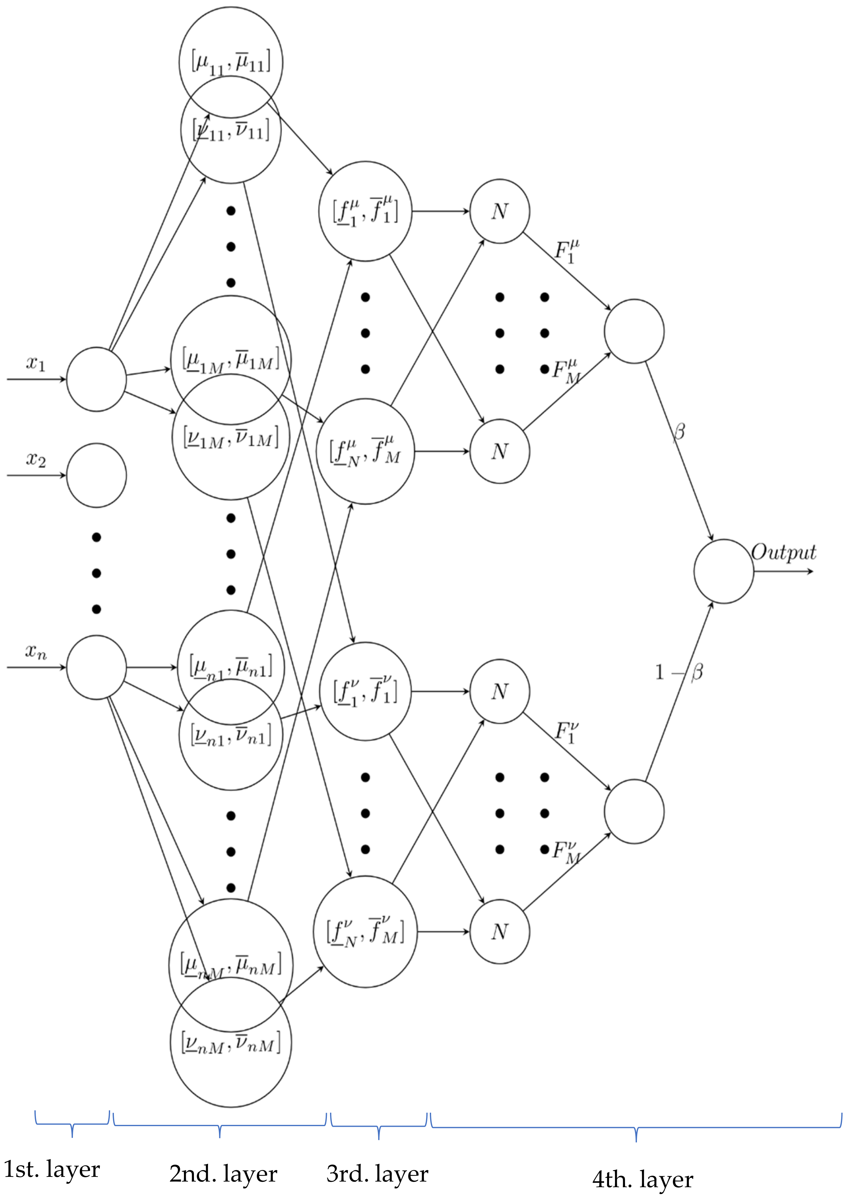
2.2. Structure of Attanassov Intutionist Fuzzy System

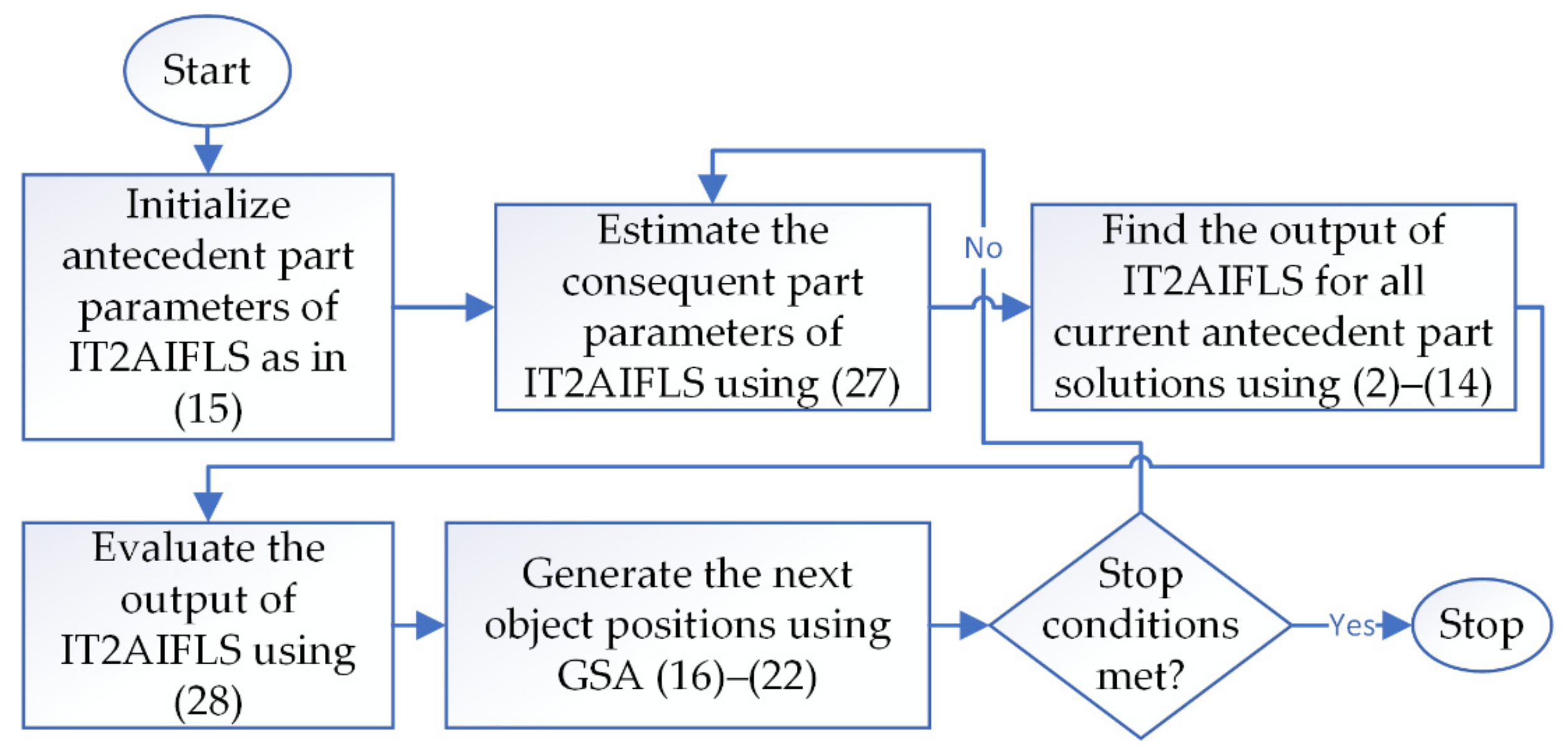
Let $T$ be the total number of inputs for the IT2AIFLS, with each sample containing $n-$dimensional input values $x\in R^n$ and $m-$dimensional output values $y\in R^m$. The membership functions considered for this structure are interval type-2 Gaussian MFs with uncertain $\sigma$ values. The inference mechanism to calculate the output of the IT2AIFLS is demonstrated in Figure 1 and is explained as follows:

Layer 1: The input layer is the first layer of this system which consists of $n$ nodes passing input values to the fuzzification layer.

Layer 2: The fuzzification layer is the second layer which uses interval type-2 Atanassov membership functions. The inputs to this layer are the outputs of the previous layer and its outputs are the degrees of membership and non-membership which are themselves interval values. The ${\pi }_{c,ik}\left(x_i\right)$ represents the IF-index or hesitation of center and ${\pi }_{var,ik}\left(x_i\right)$ is the IF-index of variance and are defined by:

$$\begin{array}{c}{\pi }_c\left(x\right)=max\left(0,\left(1-\left({\mu }_{\tilde{A}*}\left(x\right)+{\nu }_{\tilde{A}*}\left(x\right)\right)\right)\right)\\ {\underset{\_}{\pi }}_{var}\left(x\right)=max\left(0,\left(1-\left({\underset{\_}{\mu }}_{\tilde{A}*}\left(x\right)+{\overline{\nu }}_{\tilde{A}*}\left(x\right)\right)\right)\right)\\ {\overline{\pi }}_{var}\left(x\right)=max\left(0,\left(1-\left({\overline{\mu }}_{\tilde{A}*}\left(x\right)+{\underset{\_}{\nu }}_{\tilde{A}*}\left(x\right)\right)\right)\right)\end{array}$$

(3)

such that 0 ≤ π_c (x)≤ 1, 0 ≤ ▁π_var (x) ≤ 1 and 0 ≤ ¯π_var (x) ≤ 1 and the degrees of membership as well as non-membership are defined as follows:

$$\begin{array}{c}{\overline{\mu }}_{ik}\left(x_i\right)=exp\left(\frac{{(x_i-c_{ik})}^2}{2{\sigma }_{2,ik}^2}\right)\left(1-{\pi }_{c,ik}\left(x_i\right)\right), i=1,\dots ,n, k=1,\dots ,M\\ {\underset{\_}{\mu }}_{ik}\left(x_i\right)=exp\left(\frac{{(x_i-c_{ik})}^2}{2{\sigma }_{1,ik}^2}\right)\left(1-{\pi }_{c,ik}\left(x_i\right)\right), i=1,\dots ,n, k=1,\dots ,M\\ {\overline{\nu }}_{ik}\left(x_i\right)=\left(1-{\overline{\pi }}_{var,ik}\left(x_i\right)\right)-\left[exp\left(\frac{{(x_i-c_{ik})}^2}{2{\sigma }_{1,ik}^2}\right)\left(1-{\pi }_{c,ik}\left(x_i\right)\right)\right], i=1,\dots ,n, k=1,\dots ,M\\ {\underset{\_}{\nu }}_{ik}\left(x_i\right)=\left(1-{\underset{\_}{\pi }}_{var,ik}\left(x_i\right)\right)-\left[exp\left(\frac{{(x_i-c_{ik})}^2}{2{\sigma }_{2,ik}^2}\right)\left(1-{\pi }_{c,ik}\left(x_i\right)\right)\right], i=1,\dots ,n, k=1,\dots ,M\end{array}$$

(4)

The parameters ${\overline{\sigma }}_{2i,k}$, ${\underset{\_}{\sigma }}_{1i,k}$, ${\pi }_{c,ik}$, ${\pi }_{var,ik}$ and $c$ are premise part parameters associated with interval type-2 intuitionistic fuzzy MFs. Furthermore, n is the number of inputs to the system and M is the total number of rules in the fuzzy system.

Layer 3: The rule layer is the third layer of the IT2AIFLS which calculates the firing values of the rules of the fuzzy system are presented by [12]:

$$\begin{array}{c}{\overline{f}}_k^{\mu }\left(x\right)={\overline{\mu }}_{1k}\left(x_1\right)\ast {\overline{\mu }}_{2k}\left(x_2\right)\ast \dots \ast {\overline{\mu }}_{nk}\left(x_n\right)\\ {\underset{\_}{f}}_k^{\mu }\left(x\right)={\underset{\_}{\mu }}_{1k}\left(x_1\right)\ast {\underset{\_}{\mu }}_{2k}\left(x_2\right)\ast \dots \ast {\underset{\_}{\mu }}_{nk}\left(x_n\right)\\ {\overline{f}}_k^{\nu }\left(x\right)={\overline{\nu }}_{1k}\left(x_1\right)\ast {\overline{\nu }}_{2k}\left(x_1\right)\ast \dots \ast {\overline{\nu }}_{nk}\left(x_n\right)\\ {\underset{\_}{f}}_k^{\nu }\left(x\right)={\underset{\_}{\nu }}_{1k}\left(x_1\right)\ast {\underset{\_}{\nu }}_{2k}\left(x_2\right)\ast \dots \ast {\underset{\_}{\nu }}_{nk}\left(x_n\right)\end{array}$$

(5)

Layer 4: The output layer is the last layer of the system which performs the defuzzification + type reduction and calculates the output of the fuzzy system as follows.

$$y=\frac{\beta {\sum }_{k=1}^M\left({\underset{\_}{f}}_k^{\mu }+{\overline{f}}_k^{\mu }\right)F_k^{\mu }}{{\sum }_{k=1}^M{\underset{\_}{f}}_k^{\mu }+{\sum }_{k=1}^M{\overline{f}}_k^{\mu }}+\frac{\left(1-\beta \right){\sum }_{k=1}^M\left({\underset{\_}{f}}_k^{\nu }+{\overline{f}}_k^{\nu }\right)F_k^{\nu }}{{\sum }_{k=1}^M{\underset{\_}{f}}_k^{\nu }+{\sum }_{k=1}^M{\overline{f}}_k^{\nu }}$$

(6)

where the parameter $\beta \in \left[0,1\right]$ is the coefficient which determines the weight of its corresponding terms in the output. Moreover, the firing of the rules corresponding to the membership functions are defined as follows:

$$r_k^{\mu }=\frac{{\underset{\_}{f}}_k^{\mu }+{\overline{f}}_k^{\mu }}{{\sum }_{k=1}^M{\underset{\_}{f}}_k^{\mu }+{\sum }_{k=1}^M{\overline{f}}_k^{\mu }}$$

(7)

and the ones corresponding to non-membership values are defined as follows:

$$r_k^{\nu }=\frac{{\underset{\_}{f}}_k^{\nu }+{\overline{f}}_k^{\nu }}{{\sum }_{k=1}^M{\underset{\_}{f}}_k^{\nu }+{\sum }_{k=1}^M{\overline{f}}_k^{\nu }}$$

(8)

Furthermore, $F_k^{\mu }$ and $F_k^{\nu }$ are defined as follows:

$$\begin{gathered} F_k^{\mu }=\sum _{i=1}^n{\alpha }_{ik}^{\mu }{x}_i+{\beta }_k^{\mu } \\ {F}_k^{\nu }=\sum _{i=1}^n{\alpha }_{ik}^{\nu }{x}_i+{\beta }_k^{\nu } \end{gathered}$$

(9)

The output of the IT2AIFLS can be rewritten as follows [25]:

$$y=\frac{\beta {\sum }_{k=1}^M{r}_k^{\mu }{F}_k^{\mu }}{{\sum }_{k=1}^M{r}_k^{\mu }}+\frac{\left(1-\beta \right){\sum }_{k=1}^M{r}_k^{\nu }{F}_k^{\nu }}{{\sum }_{k=1}^M{r}_k^{\nu }}$$

(10)

The Equation (10) can be further compacted to the following form.

$$y=\beta y^{\mu }+\left(1-\beta \right)y^{\nu }$$

(11)

To be able to apply ridge least square algorithm to update the parameters of the IT2AIFLS, we need to write it as follows:

$$y=\beta {\theta }^{\mu T}{\varphi }^{\mu }+\left(1-\beta \right){\theta }^{\nu T}{\varphi }^v$$

(12)

where the parameters ${\varphi }^{\mu }$ and ${\theta }^{\mu }$ are as follows:

$$\begin{gathered} {\varphi }^{\mu }={\left[R^{\mu T} R^{\mu T}{x}_1 \dots R^{\mu T}{x}_n\right]}^T \\ {R}^{\mu }=\left[\frac{r_1^{\mu }}{{\sum }_{k=1}^M{r}_k^{\mu }} \frac{r_2^{\mu }}{{\sum }_{k=1}^M{r}_k^{\mu }} \dots \frac{r_M^{\mu }}{{\sum }_{k=1}^M{r}_k^{\mu }}\right] \\ \theta { }_{\left(n+1\right).M}^{\mu T}=\left[{\beta }_1^{\mu }, \dots , {\beta }_M^{\mu },{\alpha }_{11}^{\mu }, \dots , {\alpha }_{1M}^{\mu }, \dots ,{\alpha }_{n1}^{\mu }, \dots , {\alpha }_{nM}^{\mu }\right] \end{gathered}$$

(13)

and the parameters ${\varphi }^{\nu }$ and ${\theta }^{\nu }$ are as follows:

$$\begin{gathered} {\varphi }^{\nu }=\left[R^{\nu T} R^{\nu T}{x}_1 \dots R^{\nu T}{x}_n\right] \\ {R}^{\nu }=\left[\frac{r_1^{\nu }}{{\sum }_{k=1}^M{r}_k^{\nu }} \frac{r_2^{\nu }}{{\sum }_{k=1}^M{r}_k^{\nu }} \dots \frac{r_M^{\nu }}{{\sum }_{k=1}^M{r}_k^{\nu }}\right] \\ {\theta }_{\left(n+1\right).M}^{\nu T}=\left[{\beta }_1^{\nu },\dots ,{\beta }_M^{\nu },{\alpha }_{11}^{\nu },\dots ,{\alpha }_{1M}^{\nu },\dots ,{\alpha }_{n1}^{\nu },\dots ,{\alpha }_{nM}^{\nu }\right] \end{gathered}$$

(14)

3. Methodology

The parameters of the IT2AIFLS were estimated using the GSA and the R-LS algorithm. The GSA was used to estimate the antecedent part parameters of the IT2AIFLS which appears nonlinearly in the output of the system. The R-LS algorithm was used to estimate the consequent part parameters of the IT2AIFLS as they appeared linearly in the output. Because the GSA is initiated from multiple start points, the probability of falling into a local minimum for this algorithm is less than computational approaches, such as gradient descent, that are initiated from a single point.

3.1. GSA Optimization of Antecdent Part Parameters

The GSA was employed to optimize the antecedent part parameters which include the interval associated with sigma value $\left[\begin{array}{cc}{\sigma }_{1,ik}& {\sigma }_{2,ik}\end{array}\right]$ and the crisp center $\left(c_{ik}\right)$ of intutionist Gaussian functions in (4). Using the GSA, the antecedent part parameters were encoded in terms of the positions of particles in the GSA, with their velocity vector and acceleration terms updated using the GSA. Each solution in the GSA is defined as the particle positions in a $d-$dimensional search space representing the antecedent part parameters. The position vector associated with the GSA is as follows:

$$p^l=\left({\sigma }_{1,11}^l,\dots ,{\sigma }_{1,ik}^l,\dots ,{\sigma }_{1,nM}^l,{\sigma }_{2,11}^l,\dots ,{\sigma }_{2,ik}^l,\dots ,{\sigma }_{2,nM}^l,c_{11}^l,\dots ,c_{ik}^l,\dots ,c_{nM}^l\right), l=1,\dots ,N$$

(15)

where ${\sigma }_{1,ik}^l$, ${\sigma }_{2,ik}^l$ and $c_{ik}$ refer to antecedent part parameters as appeared in (4) which correspond to the k-th rule for i-th input and l represents the l-th solution for the particle, ${\sigma }_{2,ik}^l$ refers to ${\sigma }_2$ value as appeared in (4) corresponding to the k-th rule for i-th input and l is the solution counter. The total number of antecedent part parameters to be estimated in this case is equal to $3\times n\times M$. To evolve the antecedent part parameters according to the GSA, a mass value was assigned to each particle according to its merit, with a higher mass representing an antecedent part with a lower mean squared error and a lower mass representing a higher mean squared error. This makes the particles with worse performance move towards better particles. The mass of particles was updated and normalized at the t-th iteration as [5]:

$$M^l\left(t\right)=\frac{m^l\left(t\right)}{{\sum }_{l=1}^N{m}^l\left(t\right)}$$

(16)

where $m_i\left(t\right)$ is a non-normalized mass value corresponding to the i-th particle at iteration number $t$. The values of $m_i\left(t\right)$ represent the quality of a solution and are defined as [5]:

$$m^l\left(t\right)=\frac{f\left(p^l\right)-f_{worst}\left(t\right)}{f_{best}\left(t\right)-f_{worst}\left(t\right)}$$

(17)

where $f\left(p^{\mathrm{l}}\right)$ is the mean squared error value corresponding to $p^{\mathrm{l}}$ after estimating the consequent part parameters corresponding to $p^{\mathrm{l}}$ parameters using the R-LS algorithm. The R-LS is summarized in Section 3.3, $f_{worst}\left(t\right)$ and $f_{best}\left(t\right)$ are updated at every iteration as follows:

$$\begin{gathered} f_{worst}\left(t\right)=max{\left\{f\left(p^l\right)\right\}}_{l=1,\dots ,N} \\ {f}_{best}\left(t\right)=min{\left\{f\left(p^l\right)\right\}}_{l=1,\dots ,N} \end{gathered}$$

(18)

In each iteration, the acceleration term and velocity value must be calculated to update the position vector $p^l$. The position term in each step was updated as follows:

$$p^l\left(t+1\right)=p^l\left(t\right)+v^l\left(t+1\right)$$

(19)

where $v^l$ represents the velocity vector and was updated using the acceleration term $a^l$ as follows:

$$v^{\mathrm{l}}\left(t+1\right)=r_i{v}^{\mathrm{l}}\left(t\right)+a^{\mathrm{l}}\left(t\right)$$

(20)

where $v^{\mathrm{l}}\left(t\right)\in R^d$ represents the $d-$dimensional velocity of the particles at $t^{th}$ iteration and $r_i\in \left[0, 1\right]$ is a uniform random number. The acceleration term, $a^{\mathrm{l}}\left(t\right)$, was then updated as follows:

$$a^l\left(t\right)=\sum _{j\in \{1,\dots ,k_b\}}{r}_{j}G\left(t\right)\frac{M^l\left(t\right)\left(p^j\left(t\right)-p^{\mathrm{l}}\left(t\right)\right)}{\parallel p^l\left(t\right)-p^j\left(t\right){\parallel }^{r_p}+\epsilon }$$

(21)

where $k_b$ represents the number of best solutions selected, $\parallel .\parallel$ stands for the Euclidean norm, $\epsilon$ is a small value added to prevent division by $zero$, $r_p$ is the power considered for the Euclidean distance between two particles, $G\left(t\right)$ is the gravitational constant and $r_j\in \left[0,1\right]$ is a uniform random value. The gravitational constant was then updated at each iteration using the following equation:

$$G\left(t\right)=G_{0}exp\left(-\beta \frac{t}{t_{max}}\right)$$

(22)

where $G_0$ has a constant real value and $t_{max}$ is the maximum value of algorithm iteration.

3.2. Ridge Least Square Estimation of Consequent Part Parameters

The consequent part parameters of the IT2AIFLS were trained using the R-LS algorithm, also known as Tikhonov regularization. To be able to apply the R-LS algorithm to the consequent part parameters we needed to write them in a matrix form as in (23). Then the R-LS algorithm of (27) could be applied to estimate the consequent part parameters. The R-LS algorithm, also known as Tikhonov regularization, is the solution to the following $l_2$-norm cost function [21].

$$\underset{\theta \in R^n}{\min }\parallel \Phi \theta -Y{\parallel }_2^2+\mathsf{\lambda }\parallel \theta {\parallel }_2^2$$

(23)

where $\parallel .{\parallel }_2$ denotes the $l_2$-norm and $\mathsf{\lambda }$ is a regulation parameter. Furthermore, the parameters $\Phi$, $\theta$ and $Y$ are as follows:

$$\Phi =\left[\begin{array}{c}\begin{array}{c}\begin{array}{cc}{\varphi }_1^{\mu T}& {\varphi }_1^{\nu T}\end{array}\\ \begin{array}{cc}{\varphi }_2^{\mu T}& {\varphi }_2^{\nu T}\end{array}\end{array}\\ \begin{array}{c}⋮\\ \begin{array}{cc}{\varphi }_S^{\mu T}& {\varphi }_S^{\nu T}\end{array}\end{array}\end{array}\right]$$

(24)

$$Y=\left[\begin{array}{c}\begin{array}{c}{y}_1\\ y_2\end{array}\\ \begin{array}{c}⋮\\ y_S\end{array}\end{array}\right]$$

(25)

$$\theta =\left[\begin{array}{cc}{\theta }^{\mu T}& {\theta }^{\nu T}\end{array}\right]$$

(26)

where ${\varphi }^{\mu }$ and ${\varphi }^{\nu }$ for each sample are defined in (13) and (14), S is the total number of samples, ${\theta }^{\mu }$ and ${\theta }^{\nu }$ are defined in (13) and (14), $y_s, s=1,\dots ,S$ are the measured values. This solution to this problem prevents over-fitness and the analytical solution to the problem was obtained by:

$$\theta ={\left({\Phi }^T\Phi +\mathsf{\lambda }\mathrm{I}\right)}^{-1}{\Phi }^{T}Y$$

(27)

where $\mathrm{I}$ is the identity matrix. It was then necessary to select the parameter $\mathsf{\lambda }$ for the R-LS algorithm. Large values for $\mathsf{\lambda }$ needed to be avoided to maintain the prediction accuracy of the system. An appropriate value for this parameter was found to be 0.01 in this paper through trial and error.

3.3. Performance Measurement

Root mean squared error (RMSE), as the most common performance evaluation method, was used to illustrate the identification performance with its mathematical formula being as follows.

$$RMSE=\sqrt{\frac{1}{N}{{\displaystyle \sum }}_{t=1}^N{\left(y_{IT2AIFLS}\left(t\right)-y_{actual}\left(t\right)\right)}^2}$$

(28)

where $N$ is the number of test samples, $y_{actual}\left(t\right)$ is the actual value of the system target and $y_{IT2AIFLS}\left(t\right)$ is the output of the IT2AIFLS.

The flow chart of the proposed tuning method for the IT2AIFLS using GSA for the antecedent part parameters and the R-LS algorithm for the consequent part parameters is illustrated in Figure 2. The first step was to create the random initial population, then the consequent part parameters were estimated using R-LS according to (28). The output of the IT2AIFLS can then be calculated using Equations (2)–(14). The cost function associated with each member of the population was calculated using the RMSE Equation of (29). The GSA algorithm was then iterated for a single iteration to generate the next positions according to (16)–(22). If the stop conditions were not met, we had to iterate the algorithm until the stop condition was satisfied.

4. Simulation Results

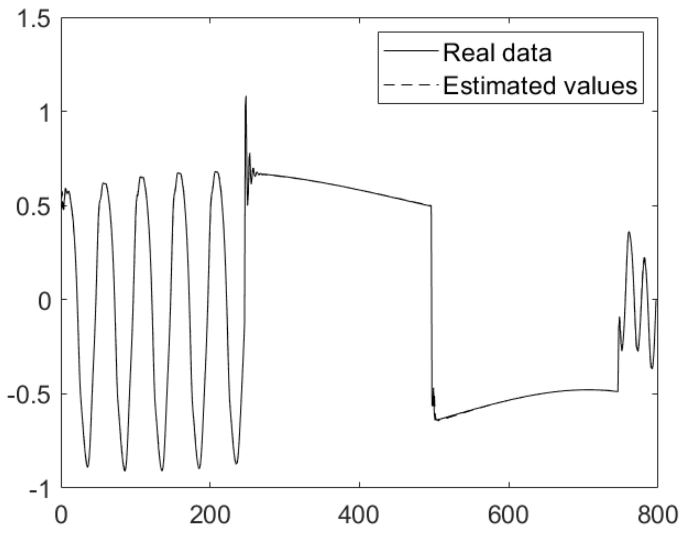
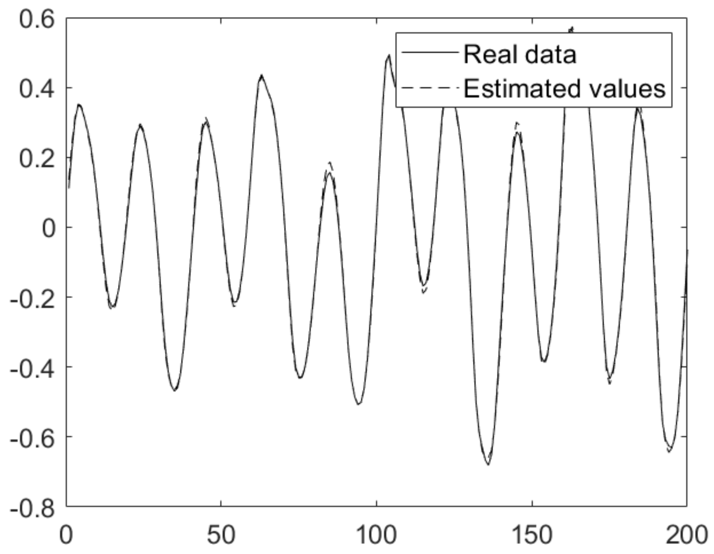
4.1. Benchmark Identification Problem

Although the proposed prediction method is mainly designed for electricity load prediction, to test its efficacy, it is implemented on a benchmark second order nonlinear dynamic system with time-varying parameters [26]. This nonlinear dynamic system has previously been tested in several papers with other prediction methods to show their efficacy. The output of this dynamic system is a nonlinear time-varying function of inputs, with time delays of input and output as follows [26].

$$y\left(t+1\right)=f(y\left(t\right),y\left(t-1\right),y\left(t-2\right),u\left(t\right),u\left(t-1\right)$$

(29)

where the nonlinear function $f\left(.\right)$ is defined as follows:

$$f\left(x_1,x_2,x_3,x_4,x_5\right)=\frac{x_1{x}_2{x}_3{x}_5\left(x_3-b\right)+c{x}_4}{a+x_2^2+x_3^2}$$

(30)

and parameters $a, b$ and $c$ are time-varying parameters defined by:

$$\begin{gathered} a\left(t\right)=1.2-0.2\cos \left(\frac{2\pi t}{T}\right) \\ b\left(t\right)=1.0-0.4\sin \left(\frac{2\pi t}{T}\right) \\ c\left(t\right)=1.0+0.4\sin \left(\frac{2\pi t}{T}\right) \end{gathered}$$

(31)

with $T$, the total number of samples, taken to be equal to 1000. The input signal to the system $u\left(t\right)$ is taken as follows:

$$u\left(t\right)=\left\{\begin{array}{c}\begin{array}{cc}\sin \left(\frac{\pi t}{25}\right) & t<250\\ 1.0& 250\le t<500.\end{array}\\ \begin{array}{cc}-1.0& 500\le t<750\\ f\left(t\right)& 750\le t<1000\end{array}\end{array}\right.$$

(32)

where:

$$f\left(t\right)=0.3\sin \left(\frac{\pi t}{25}\right)+0.1\sin \left(\frac{\pi t}{32}\right)+0.6\sin \left(\frac{\pi t}{10}\right)$$

(33)

The first 80% of the generated data is used for training and the last 20% is chosen for testing purposes. The comparison results with several other methods including Type-1 TSK FNS [27], Type-2 TSK FNS [27], Feedorward Type-2 FNN [11], SIT2FNN [28], SEIT2 FNN [29], TSCIT2FNN [30], IT2 FNN-GD [26], IT2 FNN-SMC [26], IT2 FNNPSO+ SMC [26], IT2 IFLS -DEKF+GD [11], and IT2FLS with Modified SVR [31] are presented in

Table 1. Performance of the proposed approach as well as several existing methods in the literature on time-varying system identification. Bold faced results indicate the best results.

	Rules	Epoch	Training RMSE	Testing RMSE
Type-1 TSK FNS [27]	9	100	0.0282	0.0598
Type-2 TSK FNS [27]	4	100	0.0284	0.0601
Feedorward Type-2 FNN [11]	3	100	0.0281	0.0593
SIT2FNN [28]	4	100	0.0351	0.0560
SEIT2 FNN [29]	3	100	0.0274	0.0574
TSCIT2FNN [30]	3	100	0.0279	0.0576
IT2 FNN-GD [26]	-	200	0.0540	0.0613
IT2 FNN-SMC [26]	-	200	0.0360	0.0390
IT2 FNNPSO+ SMC [26]	-	200	0.0199	0.0390
IT2 IFLS -DEKF+GD [11]	4	100	0.0250	0.0310
IT2FLS with Modified SVR [31]	11	Non-iterative	0.0146	0.0348
Proposed approach	14	200	0.0095	0.0106

,where results support the idea that the proposed approach is effective at system identification by outperforming the other tested algorithms. The behavior of the proposed identification system for the training and tesing data is presented in Figure 3 and Figure 4, respectively. As these figures show, the error between the real data and the output of the IT2AIFLS is very low.

Motivated by the fact that the proposed system identification method can successfully outperform several state-of-the-art system identification approaches in the literature, this method was then used for electrical load prediction in Section 4.2 and Section 4.3, where the real-time electrical load of Poland and five different regions in Australia are considered, respectively. Comparisons with state-of-the-art prediction models are then presented to illustrate the performance of the proposed prediction method.

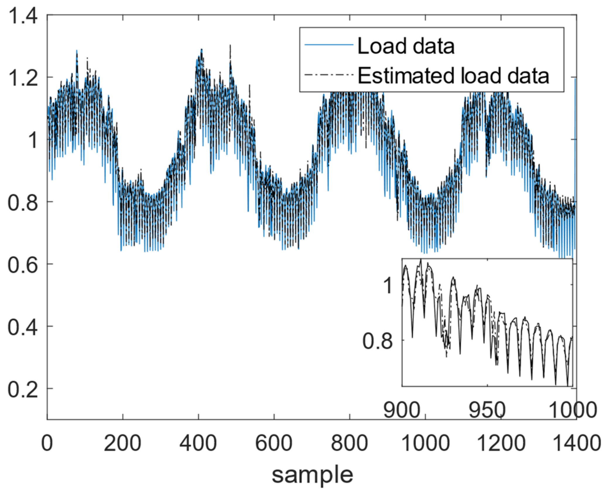
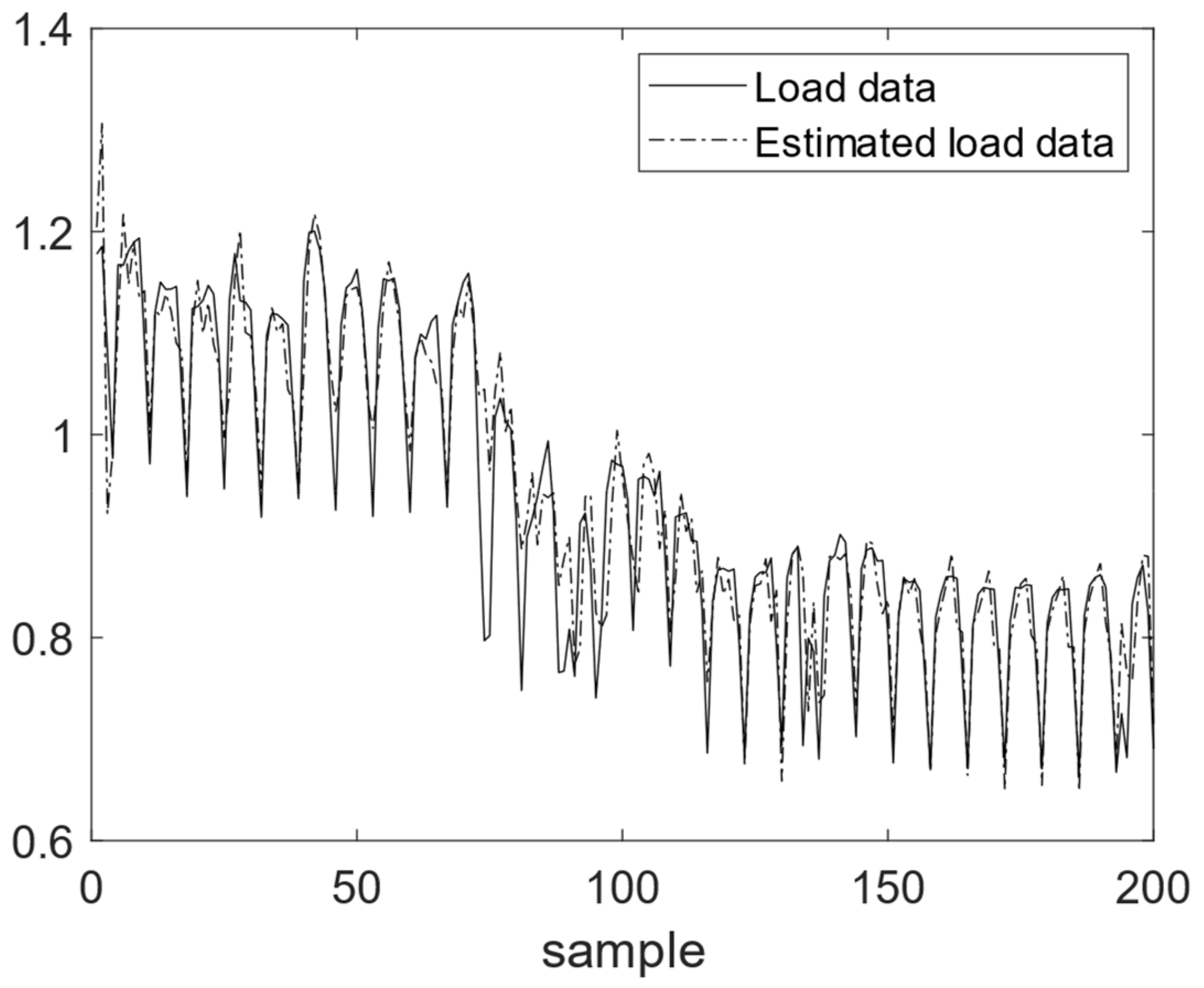
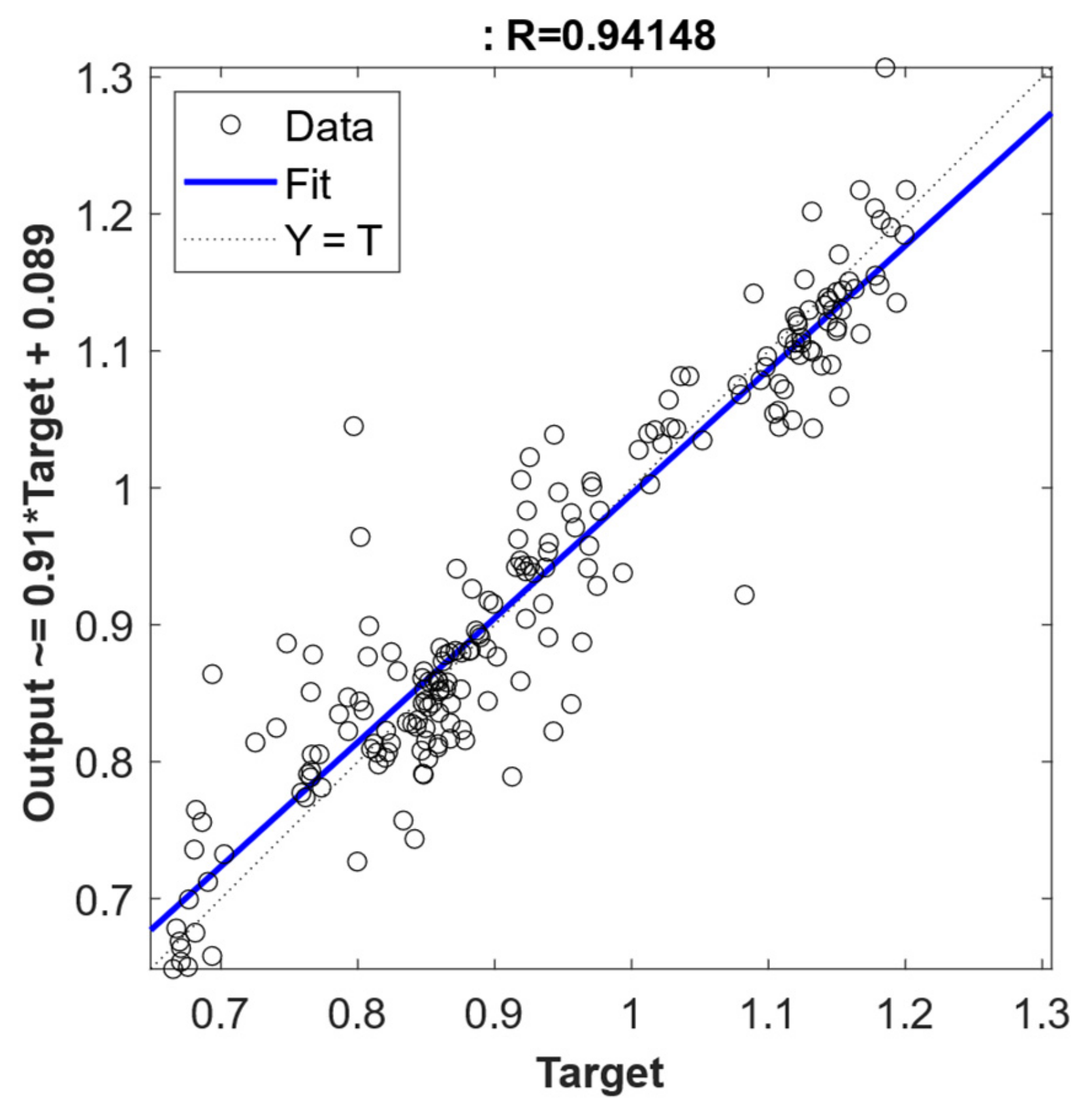
4.2. Electrical Load Prediction for Poland

The dataset selected in this part shows the performance of the proposed approach to deal with electrical load prediction using the Poland electricity load dataset available online [32] which presents electricity load values of Poland in the 1990s on a daily basis [33]. A statistical analysis is conducted for the Poland dataset to examine if this time series is stationary or not. To evaluate this property of the Poland electrical load dataset, Augmented Dickey Fuller (ADF) and Kwiatkowski–Phillips–Schmidt–Shin (KPSS) tests are utilized. These two tests are available under the statsmodels Python package. The test statistic value under these two tests as well as their critical vales are given in

Table 2. Results of the ADF and KPSS tests for the Poland electrical load dataset.

Test	Value	Critical Value (5% Confidence Interval)
ADF-test	−2.55	−2.86
KPSS-test	0.34	0.46

where it can be seen that the test value for ADF is greater than the critical value with a 5% confidence interval, and the test value for KPSS is less than the critical value with a 5% confidence interval. This means that this type of dataset is a trend stationary one. Although the stationary property of the signal is required in some statistical approaches, it is expected that the IT2AIFLS can handle this trend stationary signal due to its nonlinear nature.

As separated on the website, 1400 sample data are selected for training and 201 data samples are selected for testing. In this approach the one-step ahead prediction problem is investigated. The inputs taken for this prediction are the current value of electricity load and its time delays as $\left[y\left(t\right), y\left(t-1\right) y\left(t-2\right) y\left(t-3\right)\right].$ Here, 14 rules (number of $r_k^{\mu }$s and $r_k^{\nu }$s) are considered for the fuzzy system and the number of rules was obtained by trial and error to maximize performance. The performance comparison between the proposed approach and previous approaches in the literature are presented in

Table 3. Performance comparison of the proposed hybrid algorithm for the IT2AIFLS on the Poland electrical load dataset in terms of RMSEs. The best results are highlighted in bold.

Model	Train/Test	RMSE Train	RMSE Test
IT2FLS DEKF+GD [11]	1395/196	0.0564	0.0595
IFLS DEKF+GD [11]	1395/196	0.0589	0.0599
IT2 IFLS DEKF+GD [11]	1395/196	0.0560	0.0572
IT2AIFLS GSA-R-LS (proposed algorithm)	1395/196	0.0528	0.0501

. As can be seen from the table, IT2AIFLS with GSA-R-LS outperforms IT2FLS DEFKF+GD, IFLS DEKF+GD, IT2 IFLS DEKF+GD and IT2 AIFLS DEKF+GD (previously studied in [11] on the same dataset) by at least 5.7%. The prediction performance of the proposed algorithm for the training and testing data is presented in Figure 5 and Figure 6, respectively. As can be seen from these figures, the prediction output of the IT2AIFLS replicates the real data with high performance. The enlarged portion of the plot given in Figure 5 shows that the prediction output of the IT2AIFLS closely follows not only the low frequency part of the measured data but also the high frequency oscillations of the measured data present in the train dataset.

Figure 7 shows the regression analysis for the IT2AIFLS on the Poland electrical load dataset for test data. It can be seen that the predicted value-target value graph is close to the ideal graph of (Y = T). Furthermore, the R value for this prediction is equal to 0.94 which is close to one. Hence, the prediction is performed with high quality.

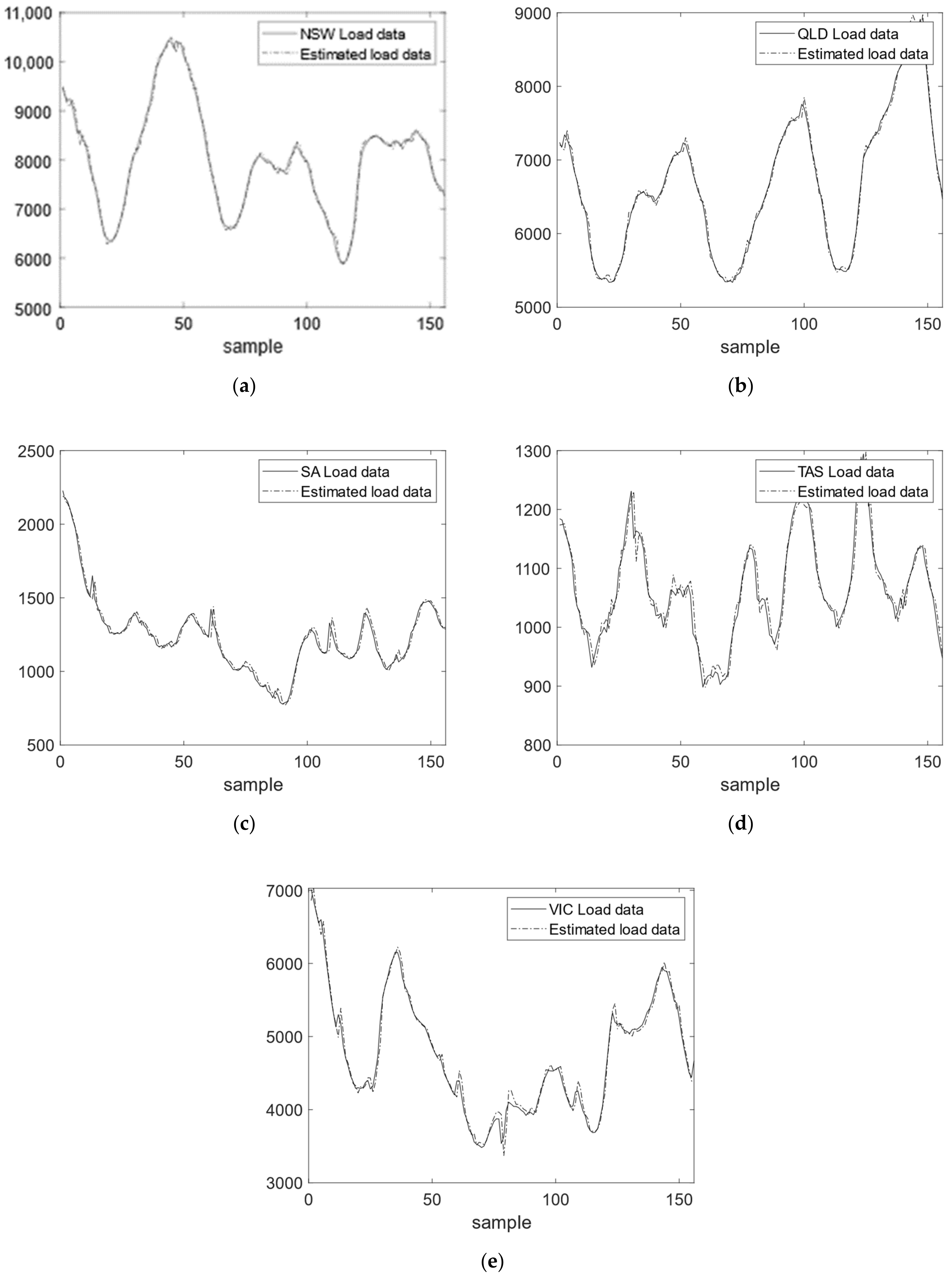
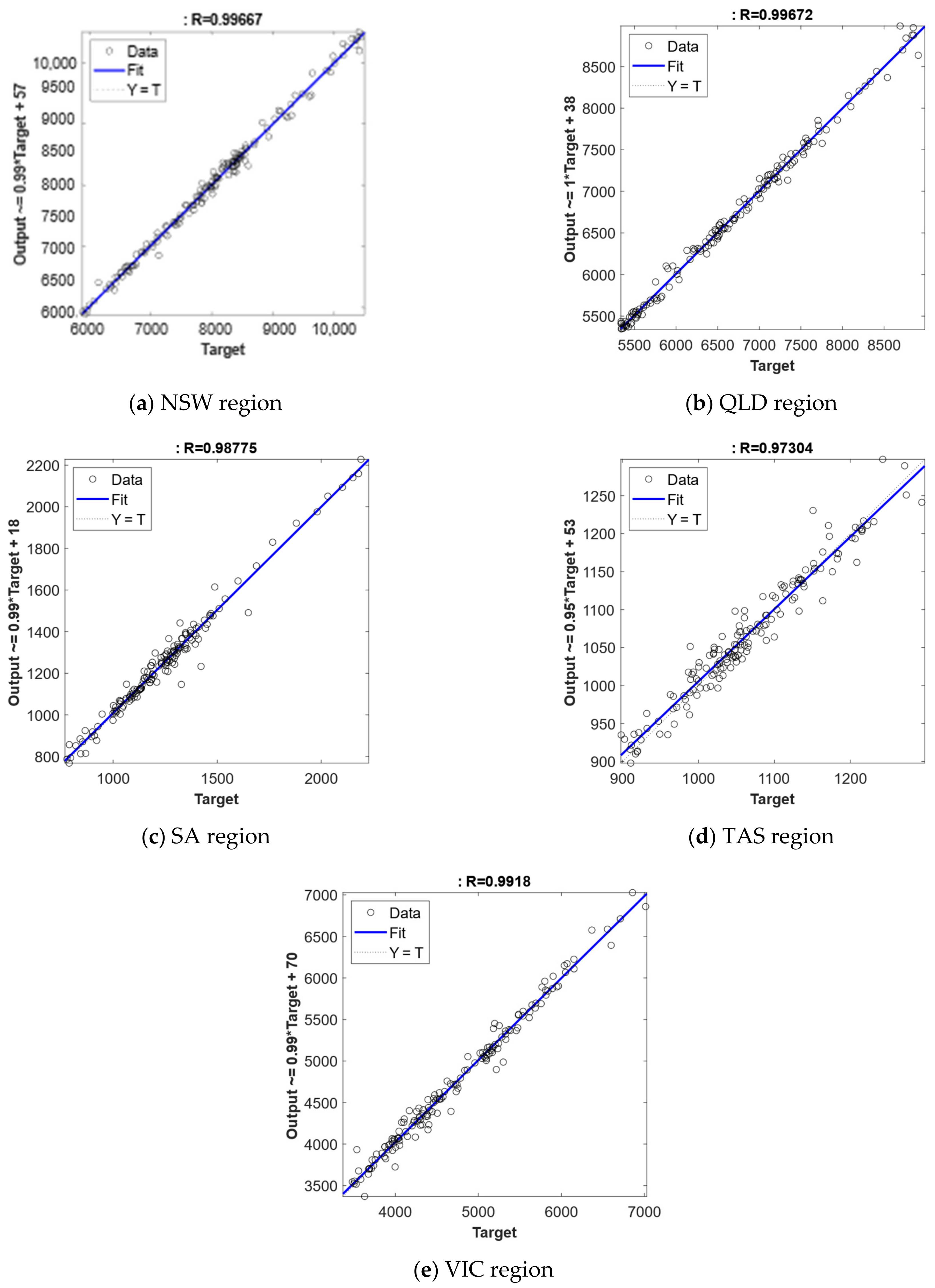
4.3. Electrical Load Prediction for Five regions in Australia

In this section, the proposed hybrid training method is used for the prediction of electrical load (MW) for five different regions in Australia, namely: New South Wales (NSW), Queensland (QLD), South Australia (SA), Tasmania (TAS) and Victoria (VIC). The datasets used in this part are retrieved from the Australian Energy Market Operator (AEMO) website at http://www.aemo.com.au (accessed on 14 June 2021). Data available on this website are available at a 30 min sample time basis. For comparison purposes, the time range of the test and train data are selected as the same as the previous study in [34]. This means that 1152 data samples from 2018/11 0:30 to 2018/2125 0:00 are used for training purposes. The data samples available from 201812/25 0:30 to 2018/2/270:00 are used for testing the prediction performance of the IT2AIFLS. The time delayed input values considered for the study are $\left[y\left(t\right), y\left(t-1\right) y\left(t-2\right) y\left(t-3\right) y\left(t-4\right)\right]$ and 14 rules are considered for the fuzzy system. The number of rules were selected via trial and error.

Table 4. Statistical parameters of the electrical load data in five regions of Australia.

	Type of Data	Number of Samples	Min	Max	Mean	Std	Skewness
NSW	Train	1152	5809.3	12846	8288	1306.7	0.35
	Test	96	5884.2	8563.3	7618.2	754.5	−0.67
QLD	Train	1152	5127.4	9480.1	6737.8	1020.5	0.73
	Test	96	5337.0	8910.9	6821.9	1060.0	0.22
SA	Train	1152	816.3	2798.0	1447.6	377.8	1.13
	Test	96	778.0	1479.8	1134.5	179.4	0.03
TAS	Train	1152	896.0	1302.1	1082.0	88.38	0.03
	Test	96	902.7	1294.1	1072.1	90.25	0.28
VIC	Train	1152	3601.6	9044.9	5049.3	927.04	1.15
	Test	96	3482.3	5945.2	4466.2	692.3	0.49

presents the statistical parameters associated with data samples which show that this dataset has high levels of variation with a large standard deviation. Furthermore, there exist some cases in Table 4 for which the Skewness value is larger than 0.5 which means that data are moderately right skewed in these cases. Example moderately right-skewed cases are the train data for QLD, the train data for SA, and the train and test data for VIC. Furthermore, the skewness for the test data in the case of the NSW region is −0.69 which is less than −0.5. This means that test data in the NSW region is moderately left-skewed. In the remaining cases, the absolute value of skewness belongs to the interval of [−0.5,0.5] which means that those datasets are fairly symmetrical.

Table 5. The result of ADF test and KPSS test for electrical load prediction of five regions of Australia.

Dataset	ADF TestValue	Critical Value (5% Confidence Interval) for ADF	KPSS Test	Critical Value (5% Confidence Interval) for KPSS	Result
NSW	−5.05	−2.86	0.45	0.46	Stationary
QLD	−6.07	−2.86	0.69	0.46	Difference stationary
SA	−3.99	−2.86	0.39	0.46	stationary
TAS	−5.95	−2.86	0.15	0.46	stationary
VIC	−4.46	−2.86	0.25	0.46	stationary

presents the results of the ADF and KPSS tests for the electrical load datasets of five regions of Australia. As Table 5 shows, the datasets associated with the electrical load for the NWS, SA, TAS and VIC regions of Australia are stationary; however, the dataset associated with the QLD region is difference stationary. Usually, it is easier to deal with stationary signals. Despite this, it is expected that the IT2AIFLS can handle difference stationary signals, where the difference of the signal is stationary, due to its nonlinear nature.

The comparison results of the proposed training algorithm for the IT2AIFLS with seven different approaches using the RMSE performance index on the test data are presented in

Table 6. Performance criteria in terms of RMSEs for electrical load prediction data in five regions of Australia (test data). The best results are highlighted in bold and MPI represents the minimum percentage improvement.

	SVR [34]	ANN [34]	ELM [34]	EEMD-ELM_GOA [34]	EEMD-ELM-DA [34]	EEMD-ELM-PSO [34]	EEMD-ELM-GWO [34]	Proposed Approach	MPI
NSW	2351	1468	1651	603	684	839	766	89	85%
QLD	905	717	705	564	336	941	558	76	77%
SA	552	380	381	154	155	261	207	41	73%
TAS	168	192	162	61	81	257	139	20	67%
VIC	1323	975	961	419	499	877	975	103	75%

. As Table 6 shows, the IT2AIFLS with the proposed training method outperforms seven other previously studied algorithms in [34], namely: SVR, ANN, ELM, EEMD-ELM-GOA, EEMD-PSO-ELM, and EEMD-ELM-GWO. The percentage improvement over these algorithms is significant and is at least 67% of improvement. Figure 8 presents plots of the prediction output of the proposed algorithm against the measured data for the electrical load data in each of the five regions of Australia. These plots show that the prediction output of the proposed algorithm closely follows the measured data which indicated that the performance of the proposed algorithm is satisfactory.

To provide greater insight on the obtained results, regression analysis is performed on the results. Figure 9 provides regression analysis for all five regions of Australia for the test data. As Figure 9 shows, the R value in all cases is very close to 1 and the bias term is reasonable. This indicates that the electrical load forecasting for five regions of Australia is performed with high quality. Moreover, although the electrical load dataset of the QLD region is a difference stationary signal, the R value obtained for it is 0.9967 which is very close to one and supports the idea that an IT2AIFLS, because of its nonlinear nature, can handle this class of data as well.

5. Conclusions

In this paper, a IT2AIFLS is trained using a hybrid method containing the GSA for the antecedent part parameters and the R-LS algorithm for consequent part parameters. A benchmark system identification problem is studied to investigate the efficacy of the proposed system parameter tuning approach on previous identification benchmark problems. The comparisons with several other methods including Type-1 TSK FNS, Type-2 TSK FNS, Feedorward Type-2 FNN, SIT2FNN, SEIT2 FNN, TSCIT2FNN, IT2 FNN-GD, IT2 FNN-SMC, IT2 FNNPSO+ SMC, IT2 IFLS -DEKF+GD, and IT2FLS with Modified SVR support the idea that the proposed approach is an efficient approach in system identification problems. The proposed approach is then investigated on electrical load prediction for five regions of Australia and Poland in the presence of noise and uncertainty which inherently exist in these datasets. Statistical properties of these datasets are presented that show they can be either stationary, trend stationary or difference stationary. In the case of the Poland electrical load dataset, the inputs to the IT2AIFLS are considered to be current values as well as three consecutive time delays of data. In the case of the five regions in Australia, current data values as well as four consecutive lags are used as the inputs to the fuzzy logic system. In both cases, one-step ahead prediction is considered. For the Poland dataset, the obtained prediction results are compared with several other algorithms including IT2FLS DEKF+GD, IFLS DEKF+GD and IT2IFLS DEKF+GD. The comparisons made in this paper show that the proposed algorithm results in superior performance when it is compared to these methods. For the case of the five regions of Australia, it is observed that the proposed prediction can perform with a much higher performance as compared with SVR, ANN, ELM, EEMD-ELM-GOA, EEMD-ELM-DA, EEMD-ELM-PSO and EEMD-ELM-GWO methods of prediction. Hence, the proposed approach is an automated solution to develop the antecedent part parameters of an IT2AIFLS, which successfully outperforms current state-of-the-art approaches in literature when applied to an electrical load prediction problem.

A possible direction of future work is the development of an interpretable IT2AIFLS which would lead to IF-THEN rules to describe the overall behavior of the electrical load system. Such IF-THEN rules are easy to communicate and may help experts to make more efficient decisions using their knowledge and experience. An additional direction of future work would be to apply the model to other time series prediction or system identification problems to test its applicability to enhance prediction in other industries.

References

1. Hassan, S.; Khosravi, A.; Jaafar, J.; Khanesar, M.A. A systematic design of interval type-2 fuzzy logic system using extreme learning machine for electricity load demand forecasting. Int. J. Electr. Power Energy Syst. 2016, 82. [Google Scholar] [CrossRef]
2. Wu, D.; Wang, B.; Precup, D.; Boulet, B. Multiple Kernel Learning-Based Transfer Regression for Electric Load Forecasting. IEEE Trans. Smart Grid 2020, 11, 1183–1192. [Google Scholar] [CrossRef]
3. Bunn, D.; Farmer, E.D. Comparative Models for Electrical Load Forecasting. John Wiley and Sons Inc.: New York, NY, USA, 1985. [Google Scholar]
4. Dutta, G.; Mitra, K. A literature review on dynamic pricing of electricity. J. Oper. Res. Soc. 2017, 68, 1131–1145. [Google Scholar] [CrossRef] [Green Version]
5. Ma, J.; Jiang, H.; Huang, K.; Bi, Z.; Man, K.L. Novel Field-Support Vector Regression-Based Soft Sensor for Accurate Estimation of Solar Irradiance. IEEE Trans. Circuits Syst. I Regul. Pap. 2017, 64, 3183–3191. [Google Scholar] [CrossRef]
6. Ma, K.; Soltani, M.; Hajizadeh, A.; Zhu, J.; Chen, Z. Wind Farm Power Optimization and Fault Ride-through under Inter-Turn Short-Circuit Fault. Energies 2021, 14, 3072. [Google Scholar] [CrossRef]
7. Ma, K.; Zhu, J.; Soltani, M.; Hajizadeh, A.; Chen, Z. Optimal power dispatch of an offshorewind farm under generator fault. Appl. Sci. 2019, 9, 1184. [Google Scholar] [CrossRef] [Green Version]
8. Jiang, Y.; Yin, S.; Dong, J.; Kaynak, O. A Review on Soft Sensors for Monitoring, Control and Optimization of Industrial Processes. IEEE Sens. J. 2020, 21. [Google Scholar] [CrossRef]
9. Contreras, J.; Espínola, R.; Nogales, F.J.; Conejo, A.J. ARIMA models to predict next-day electricity prices. IEEE Trans. Power Syst. 2003, 18, 1014–1020. [Google Scholar] [CrossRef]
10. Li, W.; Zhang, Z.G. Based on time sequence of ARIMA model in the application of short-term electricity load forecasting. In Proceedings of the 2009 International Conference on Research Challenges in Computer Science, Shanghai, China, 28–29 December 2009; pp. 11–14. [Google Scholar] [CrossRef]
11. Eyoh, I.; John, R.; de Maere, G.; Kayacan, E. Hybrid Learning for Interval Type-2 Intuitionistic Fuzzy Logic Systems as Applied to Identification and Prediction Problems. IEEE Trans. Fuzzy Syst. 2018, 26, 2672–2685. [Google Scholar] [CrossRef]
12. Member, S.; John, R. Interval Type-2 A-Intuitionistic Fuzzy Logic for Regression Problems. IEEE Trans. Fuzzy Syst. 2018, 26, 2396–2408. [Google Scholar]
13. Eyoh, I.; John, R.; de Maere, G. Interval Type-2 Intuitionistic Fuzzy Logic Systems-A Comparative Evaluation. In Proceedings of the International Conference on Information Processing and Management of Uncertainty in Knowledge-Based Systems, Cádiz, Spain, 11–15 June 2018; pp. 687–698. [Google Scholar]
14. Shoorehdeli, M.A.; Teshnehlab, M.; Sedigh, A.K. Training ANFIS as an identifier with intelligent hybrid stable learning algorithm based on particle swarm optimization and extended Kalman filter. Fuzzy Sets Syst. 2009, 160, 922–948. [Google Scholar] [CrossRef]
15. Hassan, S.; Khanesar, M.A.; Jaafar, J.; Khosravi, A. Comparative analysis of three approaches of antecedent part generation for an IT2 TSK FLS. Appl. Soft Comput. J. 2017, 51, 130–144. [Google Scholar] [CrossRef]
16. Olivas, F.; Valdez, F.; Melin, P.; Sombra, A.; Castillo, O. Interval type-2 fuzzy logic for dynamic parameter adaptation in a modified gravitational search algorithm. Inf. Sci. 2019, 476, 159–175. [Google Scholar] [CrossRef]
17. Khanesar, M.A.; Branson, D. XOR binary gravitational search algorithm. In Proceedings of the 2019 IEEE International Conference on Systems, Man and Cybernetics (SMC), Bari, Italy, 6–9 October 2019; pp. 3269–3274. [Google Scholar] [CrossRef]
18. Rashedi, E.; Nezamabadi-Pour, H.; Saryazdi, S. GSA: A gravitational search algorithm. Inf. Sci. 2009, 179, 2232–2248. [Google Scholar] [CrossRef]
19. Duman, S.; Güvenç, U.; Sönmez, Y.; Yörükeren, N. Optimal power flow using gravitational search algorithm. Energy Convers. Manag. 2012, 59, 86–95. [Google Scholar] [CrossRef]
20. Purcaru, C.; Precup, R.E.; Iercan, D.; Fedorovici, L.O.; David, R.C.; Dragan, F. Optimal robot path planning using gravitational search algorithm. Int. J. Artif. Intell. 2013, 10, 1–20. [Google Scholar]
21. Long, T.; Jiao, W.; He, G. RPC Estimation via l1-Norm-Regularized Least Squares (L1LS). IEEE Trans. Geosci. Remote Sens. 2015, 53, 4554–4567. [Google Scholar] [CrossRef]
22. Khalaf, M.M.; Alharbi, S.O.; Chammam, W. Similarity measures between temporal complex intuitionistic fuzzy sets and application in pattern recognition and medical diagnosis. Discret. Dyn. Nat. Soc. 2019, 2019, 3246439. [Google Scholar] [CrossRef] [Green Version]
23. Atanassov, K.T. On intuitionistic Fuzzy Sets Theory; Springer: Berlin/Heidelberg, Germany, 2012; Volume 283. [Google Scholar]
24. Castillo, O.; Atanassov, K. Comments on Fuzzy Sets, Interval Type-2 Fuzzy Sets, General Type-2 Fuzzy Sets and Intuitionistic Fuzzy Sets; Springer International Publishing: Cham, Switzerland, 2019; Volume 372. [Google Scholar]
25. Eyoh, I.; Eyoh, J.; Kalawsky, R. Interval Type-2 Intuitionistic Fuzzy Logic System for Time Series and Identification Problems—A Comparative Study. Int. J. Fuzzy Log. Syst. 2020, 10, 1–17. [Google Scholar] [CrossRef]
26. Kayacan, E.; Khanesar, M.A. Fuzzy Neural Networks for Real Time Control Applications: Concepts, Modeling and Algorithms for Fast Learning; Butterworth-Heinemann: Oxford, UK, 2015. [Google Scholar]
27. Abiyev, R.H.; Kaynak, O. Type 2 fuzzy neural structure for identification and control of time-varying plants. IEEE Trans. Ind. Electron. 2010, 57, 4147–4159. [Google Scholar] [CrossRef]
28. Lin, Y.Y.; Liao, S.H.; Chang, J.Y.; Lin, C.T. Simplified interval type-2 fuzzy neural networks. IEEE Trans. Neural Networks Learn. Syst. 2014, 25, 959–969. [Google Scholar] [CrossRef]
29. Juang, C.-F.; Tsao, Y.-W. A Self-Evolving Interval Type-2 Fuzzy Neural Network with Online Structure and Parameter Learning. Fuzzy Syst. IEEE Trans. 2008, 16, 1411–1424. [Google Scholar] [CrossRef]
30. Lin, Y.Y.; Chang, J.Y.; Lin, C.T. A TSK-type-based self-evolving compensatory interval type-2 fuzzy neural network (TSCIT2FNN) and its applications. IEEE Trans. Ind. Electron. 2014, 61, 447–459. [Google Scholar] [CrossRef] [Green Version]
31. Khanesar, M.A.; Branson, D.T. Prediction Interval Identification Using Interval Type-2 Fuzzy Logic Systems: Lake Water Level Prediction Using Remote Sensing Data. IEEE Sens. J. 2021, 1–13. [Google Scholar] [CrossRef]
32. Applications of Machine Learning Group. 2019. Available online: https://research.cs.aalto.fi/aml/datasets.shtml (accessed on 14 June 2021).
33. Lendasse, A.; Cottrell, M.; Wertz, V.; Verleysen, M. Prediction of electric load using Kohonen maps—Application to the polish electricity consumption. Proc. Am. Control Conf. 2002, 5, 3684–3689. [Google Scholar] [CrossRef] [Green Version]
34. Wu, J.; Cui, Z.; Chen, Y.; Kong, D.; Wang, Y.G. A new hybrid model to predict the electrical load in five states of Australia. Energy 2019, 166, 598–609. [Google Scholar] [CrossRef]
Figure 1. Structure of IT2AIFLS.
Energies 14 03591 g001
Figure 2. Flow chart of the proposed tuning method for the IT2AIFLS using the GSA for antecedent part parameters and the R-LS algorithm for the consequent part parameters.
Energies 14 03591 g002
Figure 3. Performance of the proposed prediction method for the time-varying nonlinear system dataset (train set).
Energies 14 03591 g003
Figure 4. Performance of the proposed prediction method for the time-varying nonlinear system dataset (test set).
Energies 14 03591 g004
Figure 5. Performance of the proposed prediction method for the Poland electrical load dataset (train set).
Energies 14 03591 g005
Figure 6. Performance of the proposed prediction method for the Poland electrical load dataset (test set).
Energies 14 03591 g006
Figure 7. Regression analysis for the IT2AIFLS on the Poland electrical load dataset for test data.
Energies 14 03591 g007
Figure 8. Estimation performance of the proposed prediction method for five regions of Australia electrical load dataset (train set): (a) NSW, (b) QLD, (c) SA, (d) TAS, (e) VIC.
Energies 14 03591 g008
Figure 9. Regression analysis of the proposed prediction method for five regions of Australia electrical load dataset (train set): (a) NSW, (b) QLD, (c) SA, (d) TAS, (e) VIC.
Energies 14 03591 g009