1. Introduction
The hydrostatic drivetrain, also known as hydrostatic transmission (HST), has many advantages that make it increasingly used in mobile, off-road equipment [
1]. Its advantages and development potential were indicated by [
2,
3,
4], among others. Among the most important problems that should be analyzed when designing hydrostatic driveline is power efficiency [
5,
6,
7,
8]. However, this depends on many factors, such as the structure of the system and the selection of the size of pumps and motors [
7], the method of controlling pumps and motors [
3,
8] and external loads occurring [
3,
5,
9]. In the case of the drive system, external loads mainly depend on the rolling resistance, grade resistance and drawbar load [
1,
10,
11,
12]. They must be overcome by the driving force limited by the traction capability of the wheels.
Therefore, the cooperation of the driven wheels with the ground is essential for the overall efficiency of the drive system. In order to maximize efficiency, the wheel slip should be controlled [
3,
10]. Analyses and studies [
13,
14,
15] have shown that in the case of 4 × 4 vehicles moving on soft terrain, all wheels should rotate with equal angular velocity. Otherwise, kinematic discrepancy (allowing different slips) leads to increased energy and fuel consumption. In general, kinematic discrepancy increases the resistance of the movement on hard surfaces as well [
16,
17,
18,
19,
20,
21,
22]. This means that wheels of the same diameter on flat surfaces should have the same rotational speed. Variable wheel angular velocity during straight, forward driving is recommended only when overcoming an obstacle [
16,
17,
23]. Comparative studies of heavy, multi-axle wheeled vehicles moving on soft terrain [
24,
25,
26] have shown that a properly controlled multi-pump and multi-motor hydrostatic drive can provide higher overall efficiency than a mechanical drive. Limited slip and no-spin differentials can lead to excessive slippage, reducing travel speed and decreasing the overall efficiency of a drivetrain. Ensuring proper synchronization of the angular velocity of hydraulic motors requires the use of multi-pump systems [
3,
9,
27] or the use of flow dividers [
17,
20,
21]. A flow divider, which is mounted in a drivetrain, is a hydraulic device responsible for dividing pump output flow into (an assumed) two or more equal flows into high-pressure lines of parallelly connected motors. This enables a single pump to simultaneously supply more than one parallelly connected line with different pressure values in each. Two types of flow dividers are used: the spool type and the gear type. They divide flow independent of pressure changes in circuits. In drivetrains, they are used to synchronize the angular velocity of parallelly connected hydraulic motors with unequal torque load. The flow dividing accuracy at nominal flow is about 97–98%. In the drivetrains, in order to limit the accuracy of the flow division between the circuits, e.g., during steering or overcoming obstacles, additional controlled leakage is introduced upon the operator’s request. This decreases the kinematic stiffness of the drivetrain and allows for different wheel angular velocities.
Spool dividers split the input flow proportionally into two output flows with fixed ratio. Common output ratios are 50/50, 60/40 and 66.6/33.3, but any ratio is theoretically possible. To separate flow into more than two lines, a few spools in cascade configuration should be used [
28,
29,
30,
31].
The gear-type divider can separate flow into two or more lines. A gear divider consists of a housing, two or more internal sections of mating gears and sealings that separate the sections from one another. A common shaft connects the gear sections. Fluid between the gear teeth and housing is carried around to the opposite side of the gear section. As the teeth mesh, fluid is pushed out of each outlet port. As all the gear sections are connected, all the gears rotate at the same speed. This causes this type of flow dividers to have no hysteresis during flow division. The positive displacements of the gear sections produce a constant division of the flow. Inlet flow is divided proportionally between each section [
17].
Rotary (gear) dividers have a low pressure drop across the section and many offer efficiencies approaching 98% [
32]. Spool type dividers tend to require a sizeable pressure drop just to operate. This will generate heat, and engineers need to consider the inherent inefficiency when sizing them for an application. Gear-type flow dividers are also more tolerant of contamination. Spool-type dividers, on the other hand, have little internal leakage and can be highly accurate [
33,
34].
The effectiveness of divisors depends on many factors [
17,
24]. Usually in vehicle drivetrains, they do not operate with nominal parameters. Both the pressure, which depends on the motion resistances, and the flow, which depends on the desired driving speed, can be changed within a wide range (from minimum to maximum vehicle drive speed). Moreover, even the divider operates with nominal working parameters, which means that the efficiency of the entire vehicle drive system is not at its highest. The aim of this research was to determine the impact of the type of flow divider on the total efficiency of the drivetrain at variable loads, in soft terrain, for different driving speeds.
2. Materials and Methods
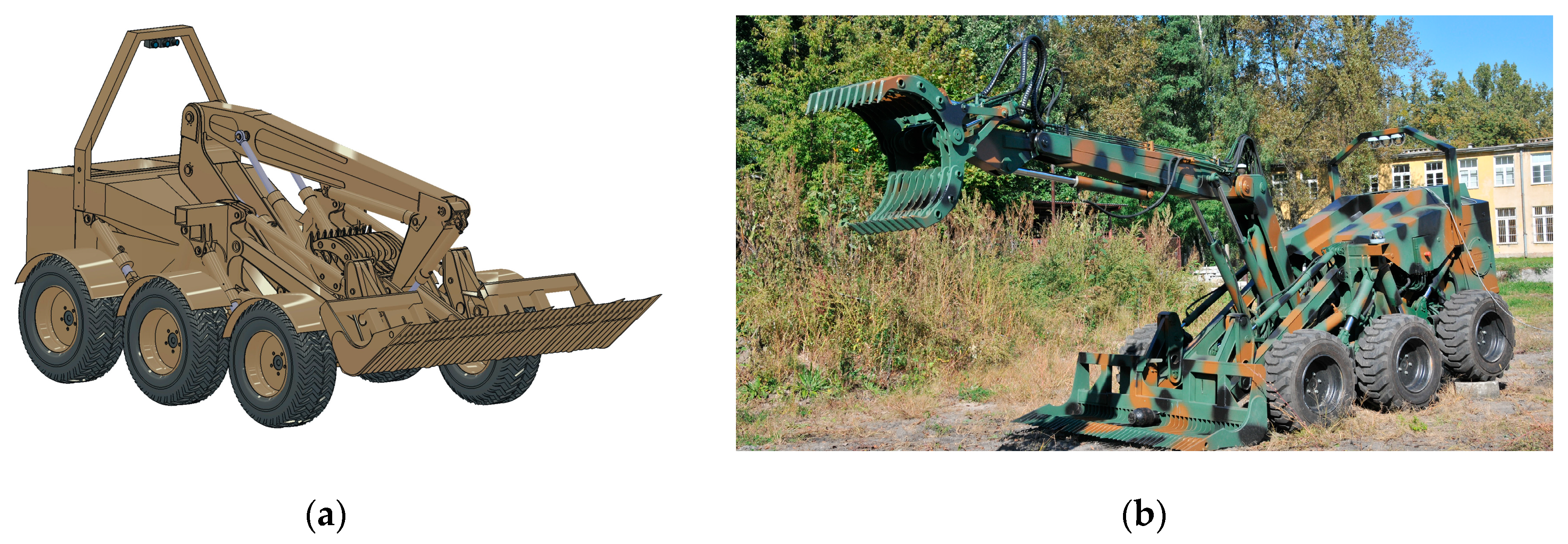
Research on the influence of the flow divider on the overall efficiency of a skid-steered all-wheel drive multiple-axle vehicle was conducted in a simulation environment. For this purpose, a co-simulation model was developed. It consists of two collaborative submodels. The first represents the mechanical structure and properties of the vehicle, and the second represents the hydrostatic drivetrain properties. The model was developed on the basis of an existing 6 × 6 skid-steered hydrostatically driven mobile robot (
Figure 1).
The robot (
Figure 1) weight is about 4 t. It is equipped with independent hydropneumatic suspension, a manipulator and a loader attachment. The robot hydrostatic drivetrain (
Figure 2) consists of variable displacement pumps (1,2) and hydraulic motors on the left (3, 4, 5) and right side (6, 7, 8) mounted directly inside the wheels. They create two independent hydrostatic transmissions, for the left and right sides of the vehicle. This configuration makes no provision for limited slip if any one of the wheels lose traction.
Research on the influence of the type of flow divider on the total efficiency of the drivetrain at variable loads, on soft terrain, for different driving speeds, was conducted with a co-simulation model consisting of two connected submodels (vehicle body model and hydrostatic drivetrain model). The combination of hydraulic and mechanical models made it possible to simulate the mutual dynamic interactions and their impact on the efficiency of the drive system.
2.1. Vehicle Body Model
A half robot (
Figure 3) was developed. It consists of three wheels driven by hydrostatic motors. The kinematic structure of the suspension system of the vehicle body model reflects the kinematics of real object suspension (
Figure 1). The total mass of the vehicle body model is half the mass of the robot.
The half vehicle model was developed with a multi-body method in Adams 2014.0.1 (MSC Software Corporation). The assumed principle of the vehicle model is shown in
Figure 4, and its parameter values are presented in
Table 1. The half vehicle body model has 3 DoF (degrees of freedom): two translational
y and
x and one rotational φ. Suspensions arms are connected (rotational) with the vehicle body at points G, H, and I. Hydropneumatics suspension components were replaced in the model with stiffness/damping elements with linear characteristics. These elements connect the arms with the body between pairs of points: A–D, B–E and C–F.
The values of masses and mass moments of inertia of particular model parts and the location of the resultant vehicle center of gravity (CM) were obtained based on the 3D–CAD vehicle model and catalog data of the main robot component manufacturers. The holonomic constraints, which were used in the vehicle model to connect its parts, were ideal (without friction).
The vehicle model uses a discrete model of a flexible wheel consisting of rigid bodies forming two circuits: the tire carcass and tire tread. The discrete elements are connected to each other and to the rim by forces and torques derived from stiffness and damping in the radial and circumferential directions; see
Figure 5.
Each rim consists of 144 elements. Thus, it meets the computational efficiency requirements in accordance with the recommendations contained in [
17].
Figure 6 shows the forces acting on the contact between the wheel and the flexible ground, which were taken into account in the developed wheel model.
Each element of the wheel tread in contact with the ground surface generates a traction force depending on the slip, the value of the traction coefficient and the normal reaction to the ground. The main wheel model parameters are presented in
Table 2.
The vertical load on the wheel is balanced by the sum of the vertical components of the elementary forces—normal and tangential—acting at the contact point of the tire with the ground (
Figure 6), which, in the developed model, was determined based on the dependence
where dR
N,i is the elementary normal reaction of the ground; dR
T,i is the elementary tangential reaction of the ground.
In agreement with the abovementioned dependence, the pulling force results from the difference in the horizontal components of normal and tangential forces acting in contact with the ground, according to
The driving force was determined according to
where φ is the traction coefficient. Hence, the driving torque is expressed as
where r
d is the wheel dynamic radius.
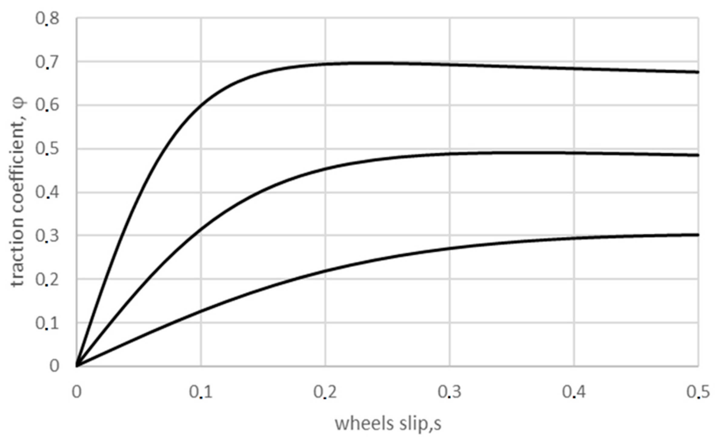
The developed model allowed us to obtain different traction coefficient values depending on slip; see
Figure 7. The dependency of traction coefficient on the slip value of the wheel model is similar to characteristics found in the literature [
15]. Slip factor is defined as ratio between theoretical wheel velocity (resulting from its angular velocity and dynamic radius) to actual velocity.
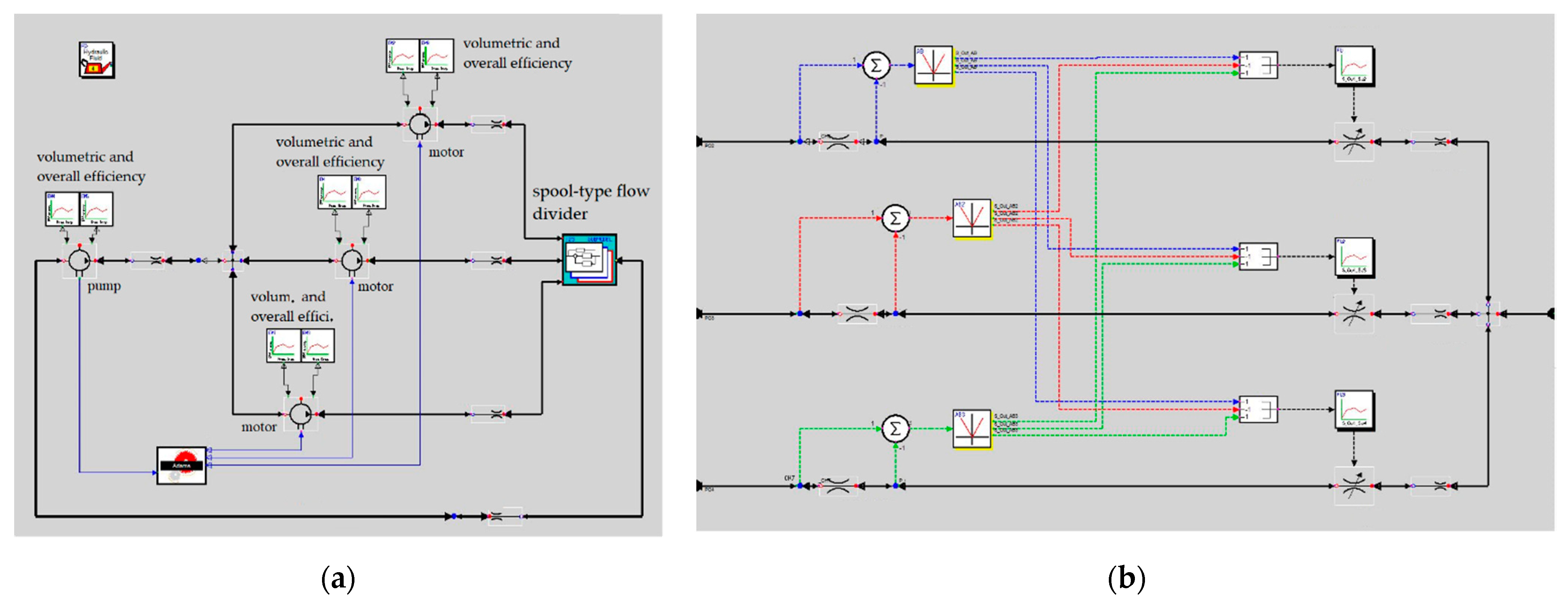
2.2. Hydrostatic Drivetrain Model
The hydrostatic drivetrain model (
Figure 8) for the half vehicle body model was developed in separate software (Easy5 2015.0.1 Version 9.1.1 (MSC Software Corporation Newport Beach, CA, USA)). To examine the impact of the flow divider properties on the overall efficiency of the hydrostatic drive system, it was necessary to modify the drive system (
Figure 2) and introduce a flow divider between the pump and hydraulic motors. The hydraulic flow divider is the unit that is responsible for equal flow division—in this case, between the hydraulic motors. The values that connect the vehicle body model and the hydrostatic drivetrain model are as follows: drive torques on the wheels
Mki and their angular velocities
ωki.
The generated driving torque
Mki by the
i-th wheel, in the model of the hydraulic drive system, caused increases in the value of the pressure drop ∆
pi on the hydraulic motor of this wheel
where
pIni is the pressure on the input of the hydraulic motor;
poi is the pressure on the output of hydraulic motor.
The pressure on the hydraulic motor input depends on the pressure drop ∆
pi and on the driving torque value
Mki
where
qs is the hydraulic motor displacement; η
os is the overall efficiency of the hydraulic motor;
ηvs is the volumetric efficiency of the hydraulic motor. The overall and volumetric efficiency of hydraulic motors depends on the motor type and value of pressure and angular velocity,
ηos,
ηvs =
f(∆
pi,
ωki), which change during vehicle driving.
The pressure
pDoi on the
i-th output of the flow divider is greater than the value
pIni shown by the pressure drop value ∆
pi resulting from flow resistance occurring on the pipes ∆
pLi and hydraulic connections ∆
pmi, which are mounted between the divider and the motor:
The pressure drop in the hydraulic pipes ∆
pLi mainly depends on the value of the friction factor
f, length
i-th pipe/hose
Li, its hydraulic diameter
DhLi, and flow velocity
VLi
where
ρ is the hydraulic oil density.
The flow velocity in the pipe/hose
Vi depends on the value of the flow rate
QDoi and hydraulic diameter
DhLiThe value of the friction factor
f depends on the of the flow character, classified on the basis of the Reynolds number
where
μ is the hydraulic oil dynamic viscosity.
For the laminar flow (
ReLi < 2000), the friction factor is calculated according to
In the case of transition state (2000 ≤
ReLi < 4000), the friction factor is calculated according to
where
f2K is the value of the friction factor calculated according to (11) for a Reynolds number value of 2000;
f4K is the value of the friction factor calculated according to (13) for a Reynolds number value of 4000.
For turbulent flow (4000 ≤
ReLi ≤
ReLiδ), the friction factor is calculated according to
where
δ is the relative roughness, whereby
For turbulent flow (ReLi > ReLiδ), the friction factor has a constant value that depends only on the value of ReLiδ calculated according to (13) for ReLi = ReLiδ.
The pressure drop occurs at the connection elements of hydraulic lines ∆
pmi, which also depends on the flow character. The laminar flow is calculated according to
where
Dh is the hydraulic diameter of the connection element;
Cd is the discharge coefficient;
ReT is Reynolds number for turbulent flow.
For turbulent flow, the pressure drop is calculated according to
Usually, to calculate the pressure drop for the connection elements, it is assumed that the transition to turbulent flow occurs at a Reynolds number of 100 (ReT = 100). Therefore, there is almost always turbulent flow.
The pressure drop between input,
pDin, and the individual output of the flow divider,
pDoi, is also calculated from (16). The pressure value,
ppo, at the pump output is higher than the pressure value,
pDin, calculated by the value of the pressure drop resulting from losses (7). The pressure drop, ∆
pp, on the pump is as follows
where
ppin is the pump input pressure, which is usually 2 MPa for closed circuit systems.
The flow rate,
Qpo, generated by the pump depends mainly on its displacement,
qp, and the angular velocity of the shaft of the engine/pump
ωs
where
ηvp is the volumetric efficiency of the pump;
ηvp =
f(∆
pp,
ωs).
The angular velocity
i-th wheel,
ωki, depends on the hydraulic motor displacement,
qs, and the flow rate,
QDoiIn line with the research aim, two hydrostatic drivetrain models were developed:
- −
One with a gear-type flow divider—
Figure 9;
- −
One with a spool-type flow divider—
Figure 10.
The main hydrostatic drivetrain model parameters are presented in
Table 3.
In the models (
Figure 9 and
Figure 10), characteristics (pump and motor volumetric, overall efficiency and flow divider’s dividing accuracy—
Figure 11) that had been identified during previously conducted laboratory research were implemented [
17]. The volumetric, total efficiency and flow divider’s dividing accuracy were identified as functions of a pressure and shaft speed map.
3. Results and Discussion
To assess the efficiency of the drive system of a vehicle with a flow divider, the main indicators were as follows:
- −
The hydrostatic transmission efficiency, calculated as
where
Ms is the torque on hydraulic pump shaft.
- −
The kinematic efficiency, calculated as
where
vj is the vehicle velocity;
rd1,
rd2, and
rd3 are the dynamic wheel radii.
- −
The overall efficiency, calculated as follows:
In order to investigate the influence of the characteristics of the flow divider used in the system on the overall efficiency of the drive transmission (22), it was assumed that the surface is flat, with a traction coefficient variable from the maximum value
μmax = 0.7 to the minimum value
μmin = 0.1 according to the following equation
where
μmax is the maximum value of the traction coefficient;
μmin is the minimum value of the traction coefficient;
l2 is the distance between the front and rear axles in a static position (
l2 = 2.1 m). The total length of the test track used in the simulation studies was
Lc = 4 ×
L2. The variation in the traction coefficient was schematic, as shown on
Figure 12.
Research was conducted with two different kinematic speeds:
vj = 0.62 m/s and
vj = 2.75 m/s. These speeds correspond to ε = 22% and ε = 100% of the pump nominal flow (
Table 3). During the simulation, the vehicle accelerated over a distance of 10 m. The kinematic speed was controlled by a setting pump flow. It was assumed that the pump shaft speed was constant during the test.
Simulation tests showed significant differences in the operation of flow dividers operating in the drive system. However, they were less noticeable when driving at speed at maximum pump capacity. The reduction in pump output and flow through the flow dividers highlighted the differences in drive efficiency. While driving with the nominal pump flow (
Figure 13a), for the spool type divider, the instantaneous driving speed decreased below 2.5 m/s, which is about 10% of the rated velocity value. In the case of the gear-type divider, the speed decreased less, by about 0.13 m/s, i.e., about 5%. While driving with 25% nominal pump flow (
Figure 13b), for the drive system with a spool flow divider, the speed drop was more pronounced and was approximately 0.3 m/s, which is approximately 50% of the speed developed on the substrate with high traction. In the case of the gear flow divider, the speed drop was approximately 0.2 m/s, which is approximately 33% of the speed developed on the surface with high traction.
Increasing the value of road wheel slip, significantly influenced the driving time. In the case of high speed and the system with a gear type divider, the driving time was approximately 7.2 s, while in the case of driving with a spool type divider, the driving time was approximately 7.7 s (more than 7% longer). While driving at a low speed with the gear divider, the driving time was about 52 s, and in the case of the spool divider, it was about 62 s—an increase of over 16%.
The imperfect work of flow dividers is very clearly visible in the graphs of angular wheel velocity. The time courses of rotational road wheels with high speed with a spool type divider are shown in
Figure 14a, while for the system with a gear divider, they are shown in
Figure 14b. As previously shown, the drive system with a spool divider allowed for a much greater differentiation of wheel angular velocities, up to a maximum of 30% compared to the average. In the case of the system with a gear divider, there were much smaller differences in the wheel angular velocities, and they amounted to a maximum of less than 5% compared to the average value.
The time courses of angular velocity changes while driving at low speed for the system with a spool divider are shown in
Figure 15a, and in the case of the gear divider arrangement, they are shown in
Figure 15b. In the case of the system with a spool divider, the influence of its non-linear characteristics is clearly visible. This non-linearity is due to the deadband in the range of small differences in flow values between the outputs connected with the hydraulic motors. As a result, within the deadband limit value of the differences in wheel rotational speed of approximately 1.7 rad/s and at low driving speed, the drive system with a spool divider enables free differentiation of the rotational speed of the wheels. Only after exceeding the limit value does the divider start to regulate the flow. The more visible the effect, the slower the speed of the vehicle. In the analyzed case, the speed differences reached 100% of the mean wheel angular velocity. This resulted in large wheel slip and a reduction in driving speed. In the case of the system with a gear divider, there is no deadband. There were much smaller differences in the angular velocity of the wheels, and they amounted to a maximum of 0.3 rad/s, which is about 17% of the average value.
The wheel torque values in the system with a spool divider are shown in
Figure 16a (high speed) and
Figure 17a (low speed), while those with the gear divider are shown in
Figure 16b (high travel speed) and
Figure 17b (low travel speed). The comparison of the torque values for both systems in the low-speed range shows that, in the system with a gear divider, there were higher maximum values of torques and greater differences between individual wheels compared to the system with a spool divider. The maximum value of the torque in the case of the system with a gear divider was about 420 Nm, and the maximum difference was 370 Nm. The value of the torque on the wheel in the low traction area dropped to about 50 Nm. In the case of the system with a spool divider, the torque on the wheels reached a maximum value of 330 Nm, and the maximum difference was 250 Nm.
The reduction in the wheel torque results from the differences in the principle of the operation of the flow dividers. In the spool divider, until the limit value of the dead zone is not exceeded, the flow is divided freely. This results in a more even distribution of driving forces on all the road wheels. When the limit value is exceeded, the divider starts throttling the flow in the wheel with the highest speed, while the other two wheels continue to adjust their speed to the load, maintaining favorable working conditions. In the presented waveforms, this is confirmed by the overlapping of the torque values. In the case of the system with a gear-type flow divider, the flow divider starts working with small differences in wheel load, increasing wheel slip. This may result in a reduction in its ability to develop driving force on the wheels in the area of low traction, and thus an increase in the load on the wheels in the area of high traction. The comparison of the values of the torque on the wheels of the systems while driving in the high-speed range showed slightly higher torque values for the system with a spool divider, which were 400 Nm, and the maximum difference between the wheels was 200 Nm. The increase in the maximum value of the torque in the case of the system with a spool divider resulted mainly from an increase in dynamic loads acting on the drive system caused by the deterioration of driving smoothness, and in turn, by the operation of the spool divider in comparison to the gear divider (gear divider operates all the time during drive).
The comparison of the pressure of the pump system for both divider types in the range of high driving speeds is shown in
Figure 18a, and in the range of low speeds in
Figure 18b. When driving at low speeds (
Figure 18b), in the case of the drive system with a spool divider, the pump pressure was higher by approximately 1.0 MPa (approximately 14%) compared to the system with a gear divider, despite having the same values of resistance to motion. The pressure difference results from higher flow resistance through the spool divider. Additionally, pressure pulsations are visible, reaching maximum values of over 8 MPa. The pump pressure in the drive system with a gear divider remained at a relatively constant level throughout the entire run. During high-speed driving (
Figure 18a), the pump pressure increased in relation to the slow speed for both systems. The maximum value of pressure in the case of the system with a spool divider was 11 MPa, while for the system with a gear divider, it was approximately 8 MPa. The pressure pulsations also increased, which, in the case of the system with a spool divider, reached 6.5 MPa, while in the case of the system with a gear divider, it reached 2 MPa. This effect was mainly influenced by the dynamic load caused by the variable value of the traction force and the increase in the hydraulic system resistance.
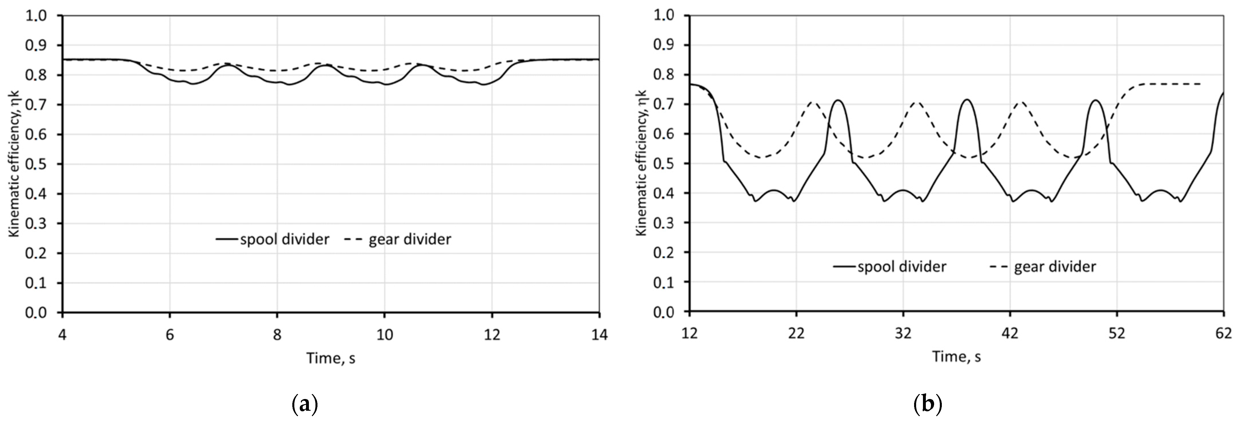
Analyzing the kinematic efficiency (
Figure 19), which depends not only on the hydraulic system but also on the interaction between the wheels and ground, it can be seen that the system with the gear divider is more efficient, both at low and high speeds. In the case of low speeds, it is in the range η
k = 0.51–0.78, while in the high-speed range, it is η
k = 0.82–0.85. In the system with a spool divider in the low-speed range, it was η
k = 0.38–0.78, while in high speed the range, it was η
k = 0.77–0.85.
The greatest differences in efficiency occurred while driving at a relatively low speed with low traction. The efficiency differences reached a value of 24%. In the case of driving at high speeds, there were much smaller differences in efficiency, and a value of about 6% was reached in favor of the system with a gear divider. The research shows that the system with a gear divider is also characterized by a higher hydrostatic transmission efficiency (
Figure 20), both in terms of low and high driving speeds. In the case of driving at low speed, the efficiency is in the range η
h = 0.55–0.60. The efficiency of the system with a spool divider in the range of low speeds is within the range η
h = 0.39–0.60, while in the range of higher speeds, it is η
h = 0.35–0.56.
The overall efficiency presented in
Figure 21a for high speed and
Figure 21b for low speed shows that the gear flow divider is much better with regard to energy. The total efficiency in the case of the system with a gear divider in the low speed range is within the range η
o = 0.40–0.59, while driving in the high speed range is η
o = 0.50–0.55. In the case of the system with a spool divider, the efficiency while driving at low speeds was η
o = 0.21–0.50, while for higher speeds, it was η
o = 0.32–0.51.
In the case of driving at low speed, the efficiency of the system with the gear flow divider is almost two times higher than that of the system with a spool divider, while when driving at high speeds, it is about 33% higher. Increasing the efficiency difference in favor of the system with a gear divider in relation to the efficiency of the system results in a more favorable cooperation of the wheels with the ground.


