Optimization of Static and Dynamic Charging Infrastructure for Electric Buses

Abstract

The adoption of electric buses in public transport requires careful planning for the bus fleet and charging infrastructure. A mathematical model of an urban bus service was developed to support the deployment of charging infrastructure. The novelty of the model is that it incorporates infrastructure elements for both static and dynamic charging technologies at the same time. The model supports the electrification of the bus lines without route and schedule adjustments. The volume of charged energy at charging units is considered as a variable in the objective function to determine the location of charging units at minimum cost. The model was verified by a case study based on actual bus service data. It was found that the use of static chargers is more favorable if the cost of a static charging unit is less than the cost of a dynamic charger with a length of 1600 m and the charging power of static chargers is three times greater than the charging power of dynamic chargers. The relationship between charging power and the length of the dynamic charging unit was analyzed. It was noted that the use of charging power higher than 162.5 kW at dynamic charging units is not necessary.

1. Introduction

The transition from conventional to pure electric drive is considered an effective way to reduce the environmental pollution of transport in urban areas [1,2]. This is no different in the public bus service, and notable actions have been made towards decarbonization. A report on the electrification of buses in the European Union revealed that 19 operators in 25 cities have a published strategy up to 2020, and more than 2500 buses should be operated by this date [3]. Albeit several electric buses are operated in Europe, it is usual that the charging infrastructure is deployed, making allowance for only a single bus line. The implemented charging infrastructure determines the electric bus service for a longer term because the payback period is very long [4]. Hence, the charging infrastructure plays a vital role in implementing electric bus service, and a well-established decision support tool is strongly recommended in charging infrastructure development. In this paper, a mathematical model of electric bus service is elaborated, which is based on charging infrastructure optimization and decision support. The aim of charging infrastructure optimization is to electrify the bus service at a minimal cost.

In contrast to electric cars, the electric buses can be charged in a stationary position (static chargers—e.g., conductive or inductive charging station) and during movement (dynamic chargers—e.g., overhead wire or inductive charging lane). The two commonly used charging technologies represent the “edges”: nighttime charging at the depot and the overhead wire power supply of trolleybuses. These solutions are not flexible enough, causing significant drawbacks. Therefore, the operational requirements, such as high availability or low sensitivity to any roadblocks along the route, cannot be met simultaneously.

Although nighttime charging can be planned efficiently, additional charging sessions should be inserted during the day because of the limited bus range. However, it is a significant barrier in operation planning. Furthermore, one charger is required for each bus. Consequently, nighttime charging is preferred in the case of a low number of electric buses. Hence, in the case of vast electric bus fleets, the use of static chargers located at terminals and stops is spreading because several buses can be served by one charging station after each other with relatively short dwelling times.

The sole use of overhead wire does not affect the maximum number of turns; however, the buses are bounded to the lines, causing spatial inflexibility. In other words, high availability can be achieved by charging during the operation time, and low sensitivity to roadblocks can be achieved by onboard energy storage. The utilization rate of static and dynamic chargers highly depends on the characteristic of the bus line. Namely, the charged energy at a charging unit is a function of the dwelling time and the number of served buses. In a complex public bus network, bus lines that are more suited to both static and dynamic chargers can be observed. Consequently, there is significant potential in using so-called combined charging infrastructure, where the static and dynamic chargers are applied jointly.

The application of mathematical models to distribute transport demand on a network with limited capacity is well-known and emerging in the field of novel transport modes as well (e.g., [5]). This paper aims to establish a model to optimize the charging of electric buses on an urban public bus network by minimizing the charging infrastructure cost without any schedule adjustment. In other words, the paper answers what charging units are to be deployed and where to serve the energy demand of buses in public transport. Thus, the electrification of bus transport can be established economically, which is crucial for decision-makers. The structure and application of the mathematical model are presented. The charging infrastructure optimization was demonstrated for a district of Budapest in Hungary as a case study.

The article proceeds as follows. Section 2 provides a brief literature overview of electric bus charging infrastructure deployment methods. In Section 3, the physical and mathematical model of the public bus service and the optimization problem to be solved are described in detail. In Section 4, the application of the mathematical model is demonstrated by the case study. In Section 5, the results are presented and discussed. In the last section, the research is concluded by emphasizing the key findings, and the future research direction is given.

2. Literature Review

Literature related to the operation of electric buses has a growing body. Most studies focus on technology [6,7], environmental aspects [8,9,10,11], energy management [12,13,14,15], and cost–benefit analysis [16,17,18]. Recently, research has been increasingly done in the field of optimal charging infrastructure deployment for electric buses. The locating problem of chargers is well-known in the field of electric cars, and it has extensive literature (e.g., [19,20,21,22,23]). Although the charging technologies of private electric cars and public electric buses have several similarities, the characteristic of the charging demand is different. This is because the public bus operates on a specific route, the stops are given, and the movements are bounded to the schedule. While the electric car patterns are usually handled separately, the entire bus fleet schedule should be considered simultaneously and not just as single turns [24]. Therefore, the charging infrastructure planning for electric buses in public transport requires a novel approach. Consequently, in the literature, we focus on the charging infrastructure of electric buses.

The studies focusing on the optimal deployment of charging infrastructure for electric buses are summarized in

Table 1. Approaches of corresponding studies.

Study	Static (1)	Dynamic (2)	Combined (3)	Network Approach (4)
Chen et al., 2018 [25]	yes	yes	no	no
Ko and Jang, 2013 [26]	no	yes	no	no
Jang et al., 2016 [27]	no	yes	no	no
Jeong et al., 2015 [28]	yes	yes	no	no
Lajunen, 2018 [29]	yes	no	no	no
Rogge et al., 2018 [30]	yes	no	no	no
Kunith et al., 2017 [31]	yes	no	no	yes
Wang et al., 2017 [32]	yes	no	no	yes
Xylia et al., 2017 [33]	yes	no	no	yes
Wu et al., 2021 [34]	yes	no	no	yes
Alwesabi et al., 2021 [35]	no	yes	no	yes
Liu and Song, 2017 [36]	yes	yes	no	yes
Bi et al., 2018 [37]	yes	no	no	yes
Wei et al., 2018 [38]	yes	no	no	yes

. The highlighted attributes of the studies are as follows: whether a certain charging technology type is considered or not (1–2); whether the combined use of charging technologies is applied or not (3); and whether the optimization is performed for a bus network or only for a single line (4).

The charging infrastructure locating studies can be categorized mainly into two groups. The papers in the first group deal with single bus lines. The battery swapping terminal, charging station, and uniformly deployed inductive wireless charging lane are compared in terms of the total cost, delay, fleet size, and battery capacity in [25]. In [26,27], the location of inductive chargers is optimized along the route of a bus line. It is revealed that the size of the bus fleet affects the location and the size of the charging infrastructure and battery capacity. The scope of stationary chargers and the developed model is extended to compare the dynamic and stationary charging in [28]. Despite the higher infrastructure cost of dynamic charging technologies, the authors found that lower battery-related costs can achieve cost saving.

Similarly, a lifecycle cost analysis of electric buses is carried out considering the nighttime and end station charging in [29]. It has been recognized that the combined use of charging technologies is recommended, and overnight chargers are not suitable for each line because of the increasing deadhead mileage. It has been observed that dynamic charging technologies are cost-competitive in transit systems with frequent service. In [30], the focus is on the relationships among the electric bus fleet composition, battery size, and frequency of charging at the depot, and the elaborated optimization model is applied to single lines. The fleet optimization is performed based on the total cost of ownership, which consists of the schedule adjustments.

The second group of papers considers the overlapping of bus routes with a network approach. Studies closer to our scope were carried out by the authors of [31,32,33,34]. They developed a public bus network model to optimize the locations of charging stations. Each paper deals with the locating problem of charging stations at terminals and stops. It is revealed that most charging stations are recommended at terminals because of the shorter dwelling times at stops.

Furthermore, the trade-off between battery capacity and charging infrastructure density affects the optimal operation significantly. The bus network and the bus fleet are integrated into a MILP model to optimize the wireless dynamic charging infrastructure in [35]. The trade-off between battery capacity and charging infrastructure cost is investigated, but the static chargers are not considered. The bus network is divided into links as candidate sites for inductive dynamic chargers considering the bus network’s characteristic in [36]. Besides, it is assumed that a charging station is located at every terminal. Thus, stationary and dynamic technologies are combined, but the locating problem of charging stations is not involved in the optimization process. As in [30], a life cycle cost analysis of stationary wireless charging stations is elaborated in [37]. Although wireless chargers can be used as dynamic chargers, this option is not considered. In [38], the scope of optimization is extended to temporal aspects. The authors focused on the deployment strategies of electric bus systems that included the locating problem of charging stations at terminals, but the dynamic charging was not considered.

It is revealed in these studies that the characteristic of a bus network (frequency, overlapping of bus lines, and average speed) affects the optimal charging solution. Furthermore, each model only considers a homogeneous charging infrastructure instead of a heterogeneous one that combines the use of static and dynamic chargers. Concerning the existing literature, the original contribution of this paper is the mathematical formalization of an optimization problem for the combined charging infrastructure of public bus service.

3. Methodology

We elaborated a model for charging infrastructure optimization to facilitate the shift to electric bus fleet. During modeling, we focused on daytime charging at static and/or dynamic chargers. In this study, daytime charging was preferred because buses may be charged during service time along the route. Thus, buses may have greater availability and lower battery capacity in comparison with nighttime charging. Furthermore, the battery swapping technology was not considered because it has a longer payback time than conventional re-charging [4].

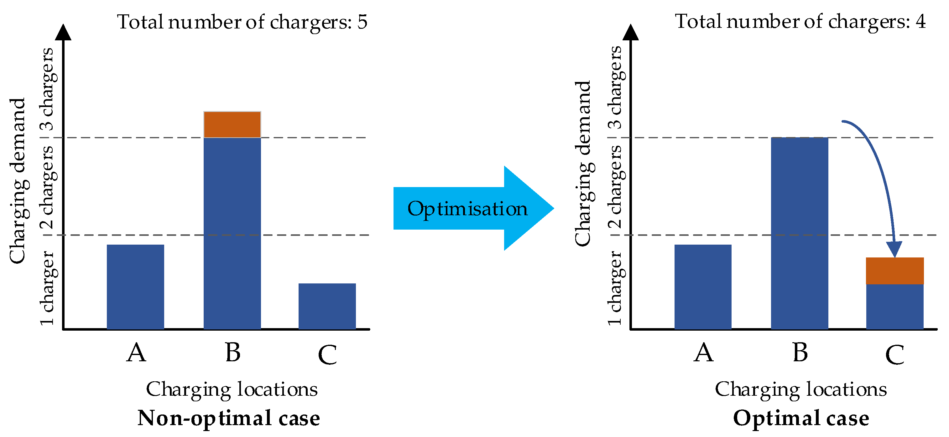
The basic idea of the modeling is to derive the optimal daytime charging infrastructure from the optimization of the volume of charged energy at charging units. The optimization of the volume of charged energy means the spatial reallocation of the charging process to minimize the total cost of charging units (Figure 1).

In Figure 1, the charging demand is served at Locations A–C. A small amount of charging demand at Location B (indicated with a different color) can be served at Location A or C. By reallocating the charging demand to Location C, the total number of chargers can be reduced by 1, while the total demand is served without any consequence in the service. On the other hand, the actual situation is much more complex, which requires a mathematical model and optimization algorithm where the deployment of a charging unit is only recommended if the charging demand does not equal zero. In other words, the total infrastructure cost is a function of the spatial distribution of charged energy.

3.1. Physical Model

Prior to building the mathematical model, first, the operational rules of the modeled bus service are defined:

• The bus fleet can be heterogeneous, but a bus line is served by one bus type. Thus, the energy consumption and charging demand is the same for each turn on a bus line.
• Three bus types are distinguished in terms of charging: a bus can be charged either at static or dynamic charging units, or both (combined bus charging).
• Each turn of a bus line begins and ends at the same station.
• The runs to and from the depot are not considered. Thus, the cost of battery capacity is not considered.
• The state of charge of a vehicle is the same at the beginning and the end of a turn. Namely, the charging process belongs exclusively to runs. There is no “additional” charging.

The rules were implemented to standardize the turns of a bus line. Therefore, the focus is on the bus line instead of the vehicle run itself. The components of the public bus service are to be modeled as follows: charging unit and bus line as well as charging processes and energy consumption. The bus network is divided into network elements that are considered as candidate sites for charging units. These elements are as follows:

• Sections: A bus line is segmented into several sections with various lengths. The division should be performed with a focus on the bus lines and branches. There is no overlap among the sections. The shorter are the sections, the greater is the number of sections. In many sections, the optimization result is more sophisticated, but the calculation takes more time. The segmentation is presented in Figure 2 with an example.

The common line section between Stop A and Stop D is segmented into two sections because of the length. Thus, the result is more sophisticated. At the branch point (Stop D), the sections should end. Namely, a branch point should not be an interior point of any section.

• Stops: Designated locations where buses frequently stop during the daily service (e.g., stop to board or alight). The energy consumption at stops is significantly smaller than during movement; accordingly, it is neglected.

Dynamic charging technology is considered at sections, and static charging technology is considered at stops. We applied the following premises to simplify the charging infrastructure during modeling:

• The cost of a charging unit is modeled by one value. This cost value may cover only the deployment cost or both the deployment cost and operational cost.
• The cost of a dynamic charger does not depend on the number of vehicles charging simultaneously.
• The vehicles are to be charged at maximum power at dynamic chargers regardless of the number of vehicles charging simultaneously.
• The cost of a static charger at a location does not depend on the number of charging units. Namely, the costs of the first and second charging stations at a specific location are equal.
• The electricity cost is the same at each location regardless the charging technology.
• The effect of electric bus technology on the charging infrastructure cost, and vice versa, were not considered. Namely, vehicles and charging units compatible with each other may be modeled.

The components and energy flows of the public electric bus service are given in Figure 3.

3.2. Mathematical Model

A deterministic model is elaborated to capture the relationships among the components of the public bus service and the cost of electrification. Stochastic factors, such as traffic congestion and weather conditions, were not considered. Thus, the modeling should be performed with safety margins. The input attributes of the cost function are summarized in

Table 2. Attributes of public electric bus service.

Component	Sign	Attribute	Description
Charging unit	cu	unit cost	Cost of a charging unit (€)
	p	power	Maximum charging power (kW)
	α	capacity coefficient	Efficiency rate because of technological specialties (connecting, reconnecting) (hour)
Energy consumption	e−	energy consumption	The consumed energy of a bus at a section during one turn (kWh)
Charging	e+	chargeable energy	The maximum energy that a bus can charge at a charging unit during one turn (kWh/turn)
	x	charged energy	The energy flow from the charging unit to the bus during one turn (kWh). The variable of the cost function.
	d	total energy demand	The total energy flow from charging unit to buses of a bus line during the rush hour (kWh/hour)
Bus line	f	frequency	The number of departures of a bus line during the rush hour (1/hour)
Technology	ct*	technology limitation factor	Its value is 0 if combined bus charging is allowed, otherwise not (€)

.

The charging infrastructure may be able to serve the peak total energy demand. Therefore, the frequency of bus lines is considered when the total energy demand on the network is the highest, i.e., during the rush hour. The attributes are considered as network element specific (c^u, p, and α), bus line specific (f), network element and bus line specific (e⁻, e⁺, x, and d), or system constant (c*) ones. Charging unit attributes are network element specific ones because the values may depend on the location. For example, the capacity coefficient may depend on the characteristic of a terminal. Factors affecting the charging power, such as batteries’ state of charge and electrical grid capacity, were not considered. Namely, an average charging power was considered. The network element specific attributes are assigned to row vectors, the bus line specific ones are assigned to column vectors, and the network element and bus line specific attributes are assigned to matrices in the model. The variable of the cost function is x (charged energy); the other input attributes are parameters.

The charging infrastructure cost, the maximum charging power of the charging units, and the capacity coefficient are given in Equations (1)–(3), respectively. The installation cost of an existing charging unit equals 0.

$$C^u=[\begin{array}{ccc}{c}_1^u& c_j^u& c_n^u\end{array}\mid \begin{array}{cc}{c}_{n+1}^u& c_{n+m}^u\end{array}]$$

(1)

$$P=[\begin{array}{ccc}{p}_1& p_j& p_n\end{array}\mid \begin{array}{cc}{p}_{n+1}& p_{n+m}\end{array}]$$

(2)

$$\alpha =[\begin{array}{ccc}{\alpha }_1& {\alpha }_j& {\alpha }_n\end{array}\mid \begin{array}{cc}{\alpha }_{n+1}& {\alpha }_{n+m}\end{array}]$$

(3)

where:

• C^u row vector of charging infrastructure cost;
• c_j^u infrastructure cost of a charging unit at network element j;
• P row vector of charging unit power;
• p_j charging power of charging unit at network element j;
• α row vector of the capacity coefficient;
• α_j capacity coefficient of charging unit at network element j;
• n total number of line sections; and
• m total number of stops.

During one turn at a section for each bus line, the energy consumption is modeled according to Equation (4). Furthermore, the chargeable energy for each network element and bus line is recorded in Equation (5).

$$E^{-}=\left[\begin{array}{ccc}{e}_{1,1}^{-}& & e_{1,n}^{-}\\ & e_{i,j}^{-}& \\ e_{k,1}^{-}& & e_{k,n}^{-}\end{array}\right]$$

(4)

$$E^{+}=[\begin{array}{ccc}{e}_{1,1}^{+}& & e_{1,n}^{+}\\ & e_{i,j}^{+}& \\ e_{k,1}^{+}& & e_{k,n}^{+}\end{array}\mid \begin{array}{cc}{e}_{1,n+1}^{+}& e_{1,n+m}^{+}\\ & \\ e_{k,n+1}^{+}& e_{k,n+m}^{+}\end{array}]$$

(5)

where:

• $E^{-}$ matrix of energy consumption;
• $E^{+}$ matrix of chargeable energy;
• $e_{i,j}^{-}$ consumed energy of a bus on bus line i at network element j during one turn;
• $e_{i,j}^{+}$ chargeable energy of a bus on bus line i at network element j during one turn; and
• k number of bus lines.

The energy consumption of buses running on various lines may be different on the same section because of the different bus types (e.g., solo and articulated) or the number of stop-and-go. The energy consumption can be a negative value (recuperation) at downhill sections. Charging time may be considered through the amount of chargeable energy because time limitations also affect the energy transfer. For example, the dwelling time at a location and the travel time along a section determine the amount of chargeable energy. If the route of the bus line i does not contain network component j, the values of $e_{i,j}^{-}$ and $e_{i,j}^{+}$ equal 0. The total energy consumption of one bus during one turn of bus line i ($E_i^{-}$) is calculated as a row sum, according to Equation (6).

$$E_i^{-}={\displaystyle \sum _j{e}_{i,j}^{-}}$$

(6)

The combined charging of buses gives more flexibility during charging planning. If the buses are charged purely at either dynamic or static chargers, the sum of chargeable energy at line sections and stops is calculated separately. In this case, electrification is possible only if the energy demand can be served by either the dynamic or the static charging units. Therefore, in the case of buses allowing combined charging in bus line i, the electrification of the line is possible if the condition in Equation (7) is met. Otherwise, it is possible if the condition in Equation (8) is met. The bus lines where electrification is not possible are disregarded during the modeling. The state of charge was not considered between charging sessions. Therefore, the battery capacity may be higher than the total energy consumption during one turn.

$$E_i^{-}\le {\displaystyle \sum _j{e}_{i,j}^{+}}$$

(7)

$$E_i^{-}\le {\displaystyle \sum _{j=1}^n{e}_{i,j}^{+}} or E_i^{-}\le {\displaystyle \sum _{j=n+1}^m{e}_{i,j}^{+}}$$

(8)

X is introduced in Equation (9) to model the charged energy at network elements for each bus line.

$$X=\left[\begin{array}{ccc}{x}_{1,1}^{}& & x_{1,n}^{}\\ & x_{i,j}^{}& \\ x_{k,1}^{}& & x_{k,n}^{}\end{array}\mid \begin{array}{cc}{x}_{1,n+1}^{}& x_{1,n+m}^{}\\ & \\ x_{k,n+1}^{}& x_{k,n+m}^{}\end{array}\right]$$

(9)

where:

• X matrix of charged energy; and
• x_i,j charged energy of a bus on bus line i at network element j during one turn.

If combined charging of buses is not allowed and one of the conditions is not met in Equation (8), it is advised to set the associated x values to constant 0. Thus, the computing time is reduced.

Since the frequency of bus lines influences the amount of charged energy at a charging unit, the number of departures per hour is considered according to Equation (10).

$$F=\left[\begin{array}{c}{f}_1\\ f_i\\ f_k\end{array}\right]$$

(10)

where:

• F column vector of frequency; and
• f_i number of departures on bus line i per hour.

The total energy demand (D), which has been charged during the rush hour, is calculated according to Equation (11).

$$F\times X=D=\left[\begin{array}{ccc}{d}_{1,1}^{}& & d_{1,n}^{}\\ & d_{i,j}^{}& \\ d_{k,1}^{}& & d_{k,n}^{}\end{array}\mid \begin{array}{cc}{d}_{1,n+1}^{}& d_{1,n+m}^{}\\ & \\ d_{k,n+1}^{}& d_{k,n+m}^{}\end{array}\right]$$

(11)

where:

• D matrix of total energy demand; and
• d_i,j total energy demand of the operating buses on bus line i in the rush hour at network element j.

Consequently, the total energy demand of the passing buses at network element j (d_j) is given in Equation (12). The variable of the summation is the index of the bus line.

$$d_j={\displaystyle \sum _i{d}_{i,j}}={\displaystyle \sum _i\left(f_i\times x_{i,j}\right)}$$

(12)

In other words, X reflects the charged energy from the point of view of an electric bus during one turn, while D represents the total energy flow from the point of view of a charging unit during the rush hour. Since F is not constant during a day, D is a function of time.

3.3. Constraints

The charged energy at a charging unit is between 0 and the chargeable energy (Equation (13)), and the total energy demand at a network element is lower than or equal to the charging capacity (Equation (14)).

$$0\le x_{i,j}\le e_{i,j}^{+} \forall i=1\dots k \mathrm{and} \forall j=1\dots n+m$$

(13)

$$d_j\le p_j\times {\alpha }_j \forall j=1\dots n+m$$

(14)

The charging capacity is calculated by multiplying the charging power (p_j) and the charging capacity coefficient (α_j). The capacity coefficient is to be determined according to local specialties. For example, if an overhead wire can charge each simultaneously connected bus at maximum power, the capacity coefficient is infinite.

Finally, a constraint is interpreted to ensure the energy supply of a bus line in Equation (15). Namely, the total charged energy on bus line i equals or is greater than the total energy consumption. Consequently, the state of charge at the end of the turn is not lower than at the beginning. The efficiency of the drivetrain and the battery is neglected. In general, during a turn, a bus cannot be charged with more energy than its energy consumption, i.e., overcharging the onboard batteries is impossible. Therefore, the difference between charged energy and energy consumption provides a reserve charging capacity.

$${\displaystyle \sum _j{x}_{i,j}}\ge E_i^{-} \forall i=1\dots k$$

(15)

3.4. Objective Function

The objective of the optimization is to serve the energy demand at minimum charging infrastructure cost.

The cost of a charging unit at network element j equals either 0 if d_j = 0 (not recommended to be deployed) or cu if d_j > 0 (recommended to be deployed). Namely, the cost function is not continuous at 0. Since the continuous functions are handled better by the optimization algorithms, substitute charging infrastructure cost functions are interpreted for two types of chargers. Charging unit with infinite capacity is interpreted in Equation (16) and charging unit with limited capacity is interpreted in Equation (17).

$$c_j^s=\left(\frac{-1}{50d_j+1}+1\right)c_j^u$$

(16)

where $c_j^s$ is the substitute cost of a charging unit where the capacity limitation is not relevant.

$$c_j^s*=\left(\frac{-1}{50\left(d_j-\lfloor \frac{d_j}{p_j{\alpha }_j}\rfloor p_j{\alpha }_j\right)+1}+1\right)c_j^u+\lfloor \frac{d_j}{p_j{\alpha }_j}\rfloor \left(\frac{-1}{50p_j{\alpha }_j+1}+1\right)c_j^u$$

(17)

where:

• $c_j^{s*}$ substitute cost of a charging unit where the capacity limitation is relevant; and
• $p_j{\alpha }_j$ energy capacity of the charging unit.

The main difference between the substitute cost functions is presented in Figure 4.

The substitute cost functions are determined in consideration with the following aspects:

• High reserve charging capacity should be avoided. Hence, the substitute cost functions should be strictly increasing. Thus, the greater reserve charging capacity would cause a higher substitute cost value.
• It should be more beneficial to allocate extra charging demand to a network element where d ≠ 0 than “install” a new charger. Hence, the first derivative of the substitute cost functions should be strictly decreasing.
• $\underset{\sum d\to \infty }{\lim }{c}^s=c^u$ and $c_j^{s*}\left(a{p}_j{\alpha }_j\right)\cong a{c}_j^u$ if a ϵ N.
• $c^s$ and $c^{s*}$ should be equal between 0 and p_jα_j if the charging unit costs are equal.

The multiplicative inverse function was applied because it fulfills the requirements above. Furthermore:

• $c^s\left(0\right) = c^{s*}\left(0\right) = 0$. Hence, the additions of 1 are applied.
• The cost of an additional charging unit and the first unit is considered the same. Therefore, c^s* is divided into the cost of a charging unit with free capacity (left section) and the cost of charging unit (s) without free capacity (right section). In other words, the left section determines the substitute cost of the first or an additional charging unit, and its domain is between 0 and p_jα_j.
• The difference between the substitute costs and $c^u$ should be low. Hence, the multiplication by 50 was applied. Therefore, the difference between $c^s$ or $c^{s*}$ and $c^u$is less than 2% if d_j is numerically greater than 1.

The $c^s$ fits chargers such as overhead wires if we assume that each simultaneously connected bus can be charged at maximum power. The $c^{s*}$ fits to charging stations, where the capacity of a station can be multiplied by deploying several chargers.

Thus, the total charging infrastructure cost in our model is given in Equation (18).

$$C^s={\displaystyle \sum c^s}+{\displaystyle \sum c^s*}$$

(18)

The exclusion of combined bus charging technology is handled by adding a theoretical cost (cost of technology limitation (c^t)) to the charging infrastructure cost. The cost of technology limitation is calculated for each bus line, according to Equation (19).

$$c_i^t=c^{t*}{\displaystyle \sum _{j=1}^n{x}_{i,j}}{\displaystyle \sum _{j=n+1}^{n+m}{x}_{i,j}}$$

(19)

where:

• $c_i^t$ cost of technology limitation for bus line i; and
• $c^{t*}$ technology limitation factor.

The two sums express the total charged energy at dynamic and static chargers, respectively. If the combined bus charging is excluded, it should be great to significantly restrict the combined bus charging. The value of $c^{t*}$ is zero if combined bus charging on a specific line is not excluded; otherwise, it is greater than zero. If $c^{t*}$ is not equal to zero, the global minimum of c^t is there, where the combined bus charging is not realized. The total cost of technology limitation is given in Equation (20).

$$C^t={\displaystyle \sum _i{c}_i^t}$$

(20)

The objective function is given in Equation (21).

$$min(C^s(X)+C^t(X))$$

(21)

4. Case Study

The public bus service network of Kőbánya (10th district of Budapest) is selected to demonstrate the applicability of the modeling and optimization method. The selected complex network is well suited for demonstration purposes because the bus network consists of radial and ring network components with many overlapping sections. Thus, relevant use cases can be observed and investigated. The rush hour was found on weekdays between 7:00 a.m. and 8:00 a.m. Twenty-six bus lines are considered. The objective of the optimization was to determine the optimum locations of charging units in terms of charging unit and technology limitation cost without schedule adjustments where the condition in Equation (7) was met.

Certain demand-responsive bus lines that are not operated during rush hours require special treatment. In our case, Bus Line 10 is operated only during special events, and it is usually not operated during the rush hour (f = 0). Therefore, the additional charging demand will not cause higher charging infrastructure costs because fx = 0. This may lead to a situation where a charging unit should be deployed to serve the energy demand of this bus line, but its cost is not considered. Therefore, the frequency of bus lines that are not operated in the rush hour is set as higher than 0. In our case study, the frequency of Bus Line 10 is set to 1. The total energy demand of that line is low compared to other lines; hence, enough charging capacity is available to serve Bus Line 10 after the optimization.

The bus network structure with the number of buses that run during the rush hour is given in Figure 5.

The network of Kőbánya is segmented into 40 sections and 5 stops. In our case, the sections cover both directions; however, the two directions could be considered as separate sections. The segmentation was performed with a focus on the branch points. The length of the sections is between 170 and 2500 m; the average length is 935 m. The charging stations are exclusively deployed at terminals because the dwelling times at stops between terminals are low. The bus line sections outside of Kőbánya are considered as separate line sections where the deployment of dynamic chargers is not possible. The energy consumption of these lines outside of the area is assigned to an imaginary section. One of the five terminals is located outside of the investigated area; nevertheless, it was included because two bus lines terminate there. Other terminals are not involved in the investigation because of the low number of departing buses or short dwelling time.

Overhead wires and conductive chargers are considered as dynamic and static chargers, respectively. The deployment of overhead wire is impossible in seven sections because of local specialties (negative impact on cityscape). Hence, infinite cost is assigned to those sections. According to the sections where the deployment of a dynamic charger is possible, the maximum length of the dynamic charging network could be 56.37 km. The charging power of the overhead wire is set as 100 kW, which is suggested in [28] as the power of a dynamic charger. The charging power of a static charger is set as 300 kW, which is the mean charging power of an OppCharger. It is assumed that an overhead wire can charge simultaneously connected buses at maximum power (α = ∞). In contrast, the capacity of a static charger is limited because of the connecting and disconnecting times at a charging session. Thus, α = 0.7 h is considered; namely, a charging station can be used 42 min per hour.

Solo and articulated buses with either static or dynamic charging are considered to demonstrate the novelty of the method. Since the elevation is not significant in Kőbánya, the lie of the land is disregarded. Therefore, constant 1.2 and 1.5 Wh/m energy consumption values were applied for solo and articulated buses, respectively. Although the average speed affects the energy consumption and may differ along various sections, it was not considered because of the lack of information on speed.

To determine the chargeable energy, the charging power was multiplied by the time spent at the network element given by the schedule. The effective charging time at the charging stations is calculated as the total dwelling time minus 1.5 min operational time (connect to and disconnect from charging station). The schedule also gives the frequency of bus lines. The total energy demand on the network is 2300 kWh in the rush hour. Some of the bus lines can be served only by static chargers because the sections do not cover its route within the investigated area, and dynamic charging units cannot serve the energy demand. Other lines can be served only by dynamic chargers because of the lack of dwelling time at terminals, or their terminals are outside of the investigated area. Therefore, the minimum energy demand on the static and dynamic charging infrastructure is 640 and 700 kWh, respectively (strict demand). In other words, 960 kWh energy demand can be served by either a static or a dynamic charger (flexible demand). In the case of strict demand, the x variables associated with the inadequate charging technology set to a constant 0. For example, Bus Line 68 can be served only by dynamic chargers. Therefore, ∀x_68,j = 0 for j = 41–45 (at terminals).

The cost of the static charger was set to €200,000 regardless of the location, while the cost of technology limitation was set to €100,000. It is expected that such high c^t eliminates the combined charging of buses successfully.

Two scenarios were analyzed.

• Without existing charging infrastructure.
• With existing dynamic charging infrastructure along a bus line because trolleybus services are spread in several European cities.

The cost of the dynamic charger was different for each optimization run to analyze its effect on the recommended charging infrastructure. Without existing charging infrastructure, the following analyses were made:

• A sensitivity analysis was made to reveal the relationship between the total length of the dynamic charging network and the charging power of dynamic charging units.
• The utilization of charging units was analyzed to validate the optimization.

The total length of the existing dynamic charging infrastructure was 13.6 km. The c^u of the existing charging infrastructure was €0. We hypothesized that the deployment of additional dynamic chargers would be more beneficial because of the existing dynamic charging infrastructure even though the cost is higher. The modeling parameters are summarized in

Table 3. Charging infrastructure parameters.

Parameter	Component	Value
cu	static charger	€200,000
	dynamic charger	different for each optimization run, 50–250 €/m
p	static charger	300 kW
	dynamic charger	100 and 100–200 kW during sensitivity analysis
α	static charger	0.7 h
	dynamic charger	infinite
e−	solo bus	1.2 Wh/m
	articulated bus	1.5 Wh/m
e+		according to the schedule and charging power
f		number of departures in rush hour
ct*		€100,000

.

The interior-point with multiple random start points and genetic optimization algorithm of MATLAB R2018b (MathWorks, Natick, MA, USA) was compared, and the interior-point was found to be more appropriate in this case according to the early optimization results. Therefore, further adjustments are only made to the interior-point algorithm. The adjustments in the optimization algorithm (such as changing the number of iterations, number of function evaluations, and the number of starting points, termination tolerance) implies the implementation of several tests, which are not shown here. All optimizations were run on a PC (Windows 10, Microsoft, Redmond, WA, USA) with Intel Core i5-6200U CPU (dual-core, 4 threads, 2.4 GHz, 8 GB DDR4 RAM). The average running time was 90 min.

5. Results and Discussion

5.1. Without Existing Charging Infrastructure

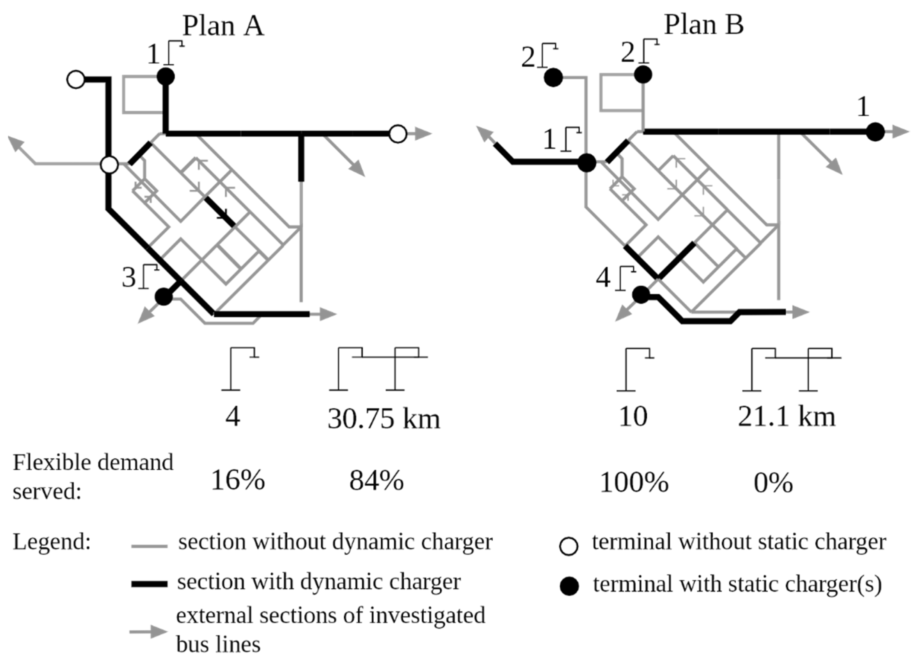
Based on the sensitivity analysis of charging infrastructure cost, two optimum charging infrastructure plans (A and B) with a cost equilibrium point were found (Figure 6).

Plan A is advised if the cost of a static charger equals €200,000 and the cost of a dynamic charger is less than 125 €/m (per direction), otherwise Plan B is more favorable than Plan A. In general, dynamic chargers are advised if the price of one static charger is enough to finance the deployment of a dynamic charger with a length of a minimum of 1600 m. Otherwise, static chargers are advised.

Four static chargers are needed to serve the strict demand. The free capacity of the proposed static chargers is used to serve flexible demand, and additional chargers are not recommended. It is assumed that transitional optima were not found between Plans A and B because of the characteristic of the bus network. Namely, the flexible energy demand can be served mainly along the same sections. Therefore, removing a section from the dynamic charging network in Plan A induces a chain reaction that results in Plan B, where static chargers serve the total flexible demand. It is noted that the units of the dynamic charging network in Plan B are not a subset of the units of dynamic charging network elements in Plan A. It also indicates the complexity of the relationship between the sections and the energy demand and the necessity of charging infrastructure optimization method.

The cost values of charging units were compared. Since the cost of charging units depends on the local characteristic, it varies in a wide range in the literature. The cost of a conductive static charger has been found to be €200,000 [4] or €250,000 [33]. Similarly, the cost of a dynamic charger in one direction is between 172 €/m (inductive charging lane [25]) and 430 €/m (inductive charging lane [28]). Considering the edges, the cost of a static unit equals the cost of a dynamic charger with a length between 465 and 1745 m. Therefore, Plan B is advised with a high probability based on the literature. However, parameters such as charging power and capacity coefficient affect the equilibrium point; it is also expected that the cost of dynamic chargers will decrease in the future. Furthermore, the charging power of static chargers in our case study was three times greater than the charging power of dynamic chargers. The higher charging power also raises its competitiveness.

The sensitivity analysis was made based on Plan A. The dynamic charging power was modified in discrete steps between 100 and 200 kW. The effect of dynamic charging power changes on the number of static charging units was not investigated. The result of the analysis is presented in Figure 7. A quasi-liner relationship between dynamic charging network length and dynamic charging power was found between 100 and 162.5 kW. The average charging network length decrement was −7.5%/10 kW. It is also noted that the charging power increment has a minor effect on the total length of the dynamic charging network if the charging power is higher than 162.5 kW. Consequently, the use of dynamic charging power greater than 162.5 kW in a complex public bus service network, such as the investigated area, is not proposed.

The length utilization rate is defined as the rate of the longest length during which a bus is being charged along the section and the total length of the section. For example, the length utilization rate is 100% if at least one bus is charged along the total length of the section. The length utilization rate is interpreted to determine the favorable section length during network segmentation.

In the case of Plan A, the average capacity utilization was 95%. This indicates that the network segmentation focusing on the branch points results in a high length utilization. However, the length utilization of sections longer than 1 km was significantly lower than the length utilization of shorter sections (90% and 97%, respectively). Therefore, it is not recommended to use sections longer than 1 km. Since the length utilization rate is not 100%, the total length of the dynamic charging network could be decreased by 2.1 km. The average length reduction was 300 m per section.

Similarly, the capacity utilization of static chargers is also high. At the terminal where three chargers are advised, the average capacity utilization is 96% and 91% at the other terminal. The high length utilization of dynamic chargers, the high capacity utilization of static chargers, and the low potential to decrease the total length of the dynamic charging network indicate that Plan A is close to the global optimum.

5.2. With Existing Dynamic Charging Infrastructure

Contrary to the hypothesis, only one optimum infrastructure plan was found regardless of the infrastructure cost of charging units (Figure 8). It is because the additional dynamic charging infrastructure components are necessary to serve the strict demand. The total length of the additional dynamic charging infrastructure is 19.8 km, which is slightly shorter than the length of dynamic infrastructure in Plan B. It is also noted that the result is a transition between Plans A and B. In other words, the existing charging units significantly affect the optimum solution, thus reducing the number of optimums.

6. Conclusions

The mathematical model of an urban public bus service network was developed focusing on the energy flow at sections and stops, which is the main contribution of the paper. The novelty of the model is that it supports the locating and combined use of static and dynamic charging infrastructure. Furthermore, the existing charging infrastructure can be considered. Hence, the trolleybus networks can be expanded cost-effectively. Furthermore, by defining several scenarios, the effect of various charging power on the number of charging units can be analyzed, and the optimal charging power can be determined.

The model was applied for a bus network in Budapest as a case study. In the case of no existing charging infrastructure, a cost equilibrium point was found between the two charging technologies. Namely, if the charging power of a static charger is three times greater than the charging power of dynamic chargers, static charging is more favorable if the cost of a charging unit is less than the cost of a dynamic charger with a length of 1600 m, which is the key finding of the paper. Comparing the cost equilibrium point to the cost values in the literature, currently, the deployment of static chargers is more beneficial. Furthermore, a quasi-linear relationship between the total length of the dynamic charging network and dynamic charging power was found between 100 and 162.5 kW. Over 162.5 kW, the charging power increment has slight effects on the total length.

The proposed infrastructure as a solution was investigated in the term of utilization. High capacity utilization is noted, which indicates that the solution was close to the global optimum. To raise the utilization and reduce the total length of the dynamic charging infrastructure, sections shorter than 1 km are advised. The optimization was also performed when an existing trolleybus line in the investigated area is assumed. It was found that the number of optimum solutions was reduced, and the charging infrastructure along a single bus line significantly influences the optimum charging infrastructure of the whole network.

In summary, the developed model is a helpful tool for determining charging infrastructure characteristics (location, number of charging stations, power) for electric buses because it handles large-scale networks instead of specific bus lines considering the characteristic of the charging technologies and the bus service.

The further direction of the research is to catch the effects of the charging infrastructure on the necessary battery capacity because its cost significantly influences the purchase price of electric buses and the complete electrification of the service. An additional objective is to model the compatibility between electric bus and charging technology because it may support the optimization of the heterogeneous bus fleet and charging infrastructure.