Article

Bin Weather Data for HVAC Systems Energy Calculations

by
Konstantinos T. Papakostas
1,*,
Dimitrios Kyrou
1,
Kyrillos Kourous
1,
Dimitra Founda
2 and
Georgios Martinopoulos
3,*
1
Department of Mechanical Engineering, Faculty of Engineering, Aristotle University of Thessaloniki, EL 54124 Thessaloniki, Greece
2
Institute for Environmental Research & Sustainable Development, National Observatory of Athens, EL 15236 Athens, Greece
3
School of Science and Technology, International Hellenic University, EL 57001 Thessaloniki, Greece
*
Authors to whom correspondence should be addressed.
Energies 2021, 14(12), 3501; https://doi.org/10.3390/en14123501
Submission received: 12 May 2021 / Revised: 4 June 2021 / Accepted: 10 June 2021 / Published: 12 June 2021
(This article belongs to the Special Issue Urban Microclimate Analysis on Buildings Energy Performance)

Abstract

:
The increase in global air temperature is well documented, as during the last several years each decade has been consecutively warmer than the preceding. As climatic conditions affect the energy performance of buildings, the changes in outdoor air temperature and humidity will inevitably lead to significant alterations in energy consumption and costs for the heating, ventilating and air conditioning (HVAC) of buildings. The availability and quality of climatic data play an important role in the accuracy of energy analysis results. In this study, the hourly temperature and relative humidity of outdoor air measurements, for a period of three decades (1983–2012), recorded at the climatic station of the National Observatory of Athens were processed, and an up-to-date set of specific data for the application of bin methods was produced and presented. The data were then used to calculate changes in the energy demands in a typical office building throughout the specified period. Results showed a progressive reduction in the low and increase in the high temperature intervals, leading to an increase in the building’s annual energy requirements for air conditioning of up to 14.5% from the first to the third decade, with decrease in the energy demands for heating and increase in the energy demands for cooling.

1. Introduction

During the last few decades it has become apparent that climate change is an imminent threat. Climate change is the shift of climate on a global scale, because of both natural processes and human activities which extend over time and can cause serious impacts on the natural ecosystem, the economy and the well-being of humanity as a whole. The effects are already apparent and are likely to intensify in the coming decades [1]. The rising average temperature of the planet, the high incidence of extreme weather and the melting glaciers in the Antarctic are just a few examples of the climate alterations that have raised the concern of the global scientific community in recent years [2].
According to the Intergovernmental Panel on Climate Change (IPCC) [1], the increase in the surface air temperature is reported and well documented on both global and regional scales, and each of the last three decades has been consecutively warmer than any preceding decade. Moreover, the National Oceanic and Atmospheric Administration (NOAA) reports that the ten warmest years on record on a global scale have occurred since 2005 [3], while the years from 2015 to 2019 are the warmest years ever recorded in NOAA’s 1880–2019 record. The year 1998 is the only year from the 20th century among the 10 warmest years on record [4]. The results of modeling studies indicate a high probability of a further air temperature rise in the future and an increase in the frequency of hot and extremely hot days, whereas extremely cold days will likely be decreased [5].
The main cause of climate change is the increased combustion of fossil fuels which releases vast amounts of CO2 into the atmosphere, which is one of the most important greenhouse gases (other than methane, nitrogen oxide and fluorinated gases) and the main culprit for global warming.
The Mediterranean region has been characterized as a “hot-spot” with respect to future heat-related risk [6], which means that impacts on sectors such as energy, biodiversity, urbanism and health are expected to be particularly pronounced in the coming years [7]. Greece is considered to be a country which will face the impact of climate change on a large scale, especially considering its geographical location (between temperate Europe and the desert of North Africa), extensive coastline and large biodiversity [1]. More specifically, by 2071–2100, Greece’s temperature is expected to rise by an average of 3.4 °C in winter and 4.5 °C in summer (compared to the 1961–1990 reference period), with an even higher increase in continental areas [5].
Presently, 41% of all energy used and 36% of CO2 emissions in Europe are attributed to the building sector, with over two thirds of them for heating and air conditioning [8]. The increase in outdoor air temperature, due to climate change and global warming, will inevitably affect the energy consumption of buildings energy systems and lead to increased costs for summer air conditioning and cooling (especially in warmer locations), while reducing the corresponding heating costs (especially in colder locations) [9]. This means that the contribution of the built environment to the overall energy consumption will be even more significant than before.
Today, the way that a building’s heating and cooling demands are dealt with has changed considerably. In the past, the interest of practitioners was mainly focused on providing thermal comfort and favorable conditions for human health in living and working areas [10]. Today, special emphasis is placed on energy savings and improved energy efficiency, in order to minimize the cost of the energy systems and their indirect environmental impacts [11].
Addressing the last two issues requires an accurate assessment of the energy needs of a building through appropriate computational methods. By accurately estimating the energy requirements of a building, it is possible to consider a variety of heating, ventilation or air conditioning (HVAC) system’s alternatives or building energy refurbishments, which can lead to both energy savings and the consequent reduction of the indirect effects of HVAC systems on the environment [12]. Energy analysis over the whole temperature range of outdoor air, by considering outdoor humidity as well, is important in the overall design of HVAC systems, which mostly operate under part load conditions, while humidity affects the latent load of ventilation and infiltration.
In this framework, in the present study, the hourly temperature and relative humidity of outdoor air measurements recorded at the climatic station of the National Observatory of Athens (NOA) [13] were statistically processed for the 1983–1992, 1993–2002 and 2003–2012 decades separately, and the following data were calculated:
(a)
The frequency (in hours) of outdoor air dry-bulb temperature, at temperature intervals of 2 °C and in six daily 4-hour shifts, for each month;
(b)
The corresponding values of the mean coincident humidity ratio at each temperature interval of 2 °C, as well as the range (maximum–minimum) of humidity ratio;
(c)
The corresponding values of the mean coincident wet-bulb temperature (MCWB) at each temperature interval; and
(d)
The average monthly ambient temperature for the three decades. The data were also integrated in three periods of the year for each decade: heating, cooling and transitional between summer and winter period.
The results are presented in diagrams and tables. Due to space limitations, only parts of them are presented in this manuscript; more analytical results are included elsewhere [14]. Scope of this work is to provide a data set, based on recent historical climatic records, which is useful for performing energy analysis of HVAC systems with simplified multiple measure methods such as the classical bin method [15,16], the modified bin method [17] and the monthly method according to ISO 52016-1:2017 [18]. Such data were published in the past [19] but are outdated because of the effects of climate change on the local climate. They present a thorough analysis of the dry-bulb temperature and humidity of the outside air for three 10-year periods and present for the first time the changes of humidity ratio and wet-bulb temperature in a 30-year period. The data presented in this work may serve to update the bin data of the Warmer zone of EN14825 [16]. Furthermore, the results indicate significant temperature variations, as well as fluctuations in the mean humidity ratio values and humidity ratio range between the three decades of the survey which provide useful insights regarding climate change during the examined period. The data are then used to calculate changes in the energy demands in a typical office building throughout the specified period, highlighting the differences in the heating and cooling loads.

2. HVAC Systems Energy Requirements Assessment

The energy consumption of an HVAC system is affected by a complex interaction between building design, system operation and the surrounding environment. It depends on many factors, among which the most important are the local climate, the typology and the energy design of the building in which it is installed. Also of significance are the influence of the occupants’ presence and behavior characteristics, the use of lights, electrical and electronic devices, the efficiency of the HVAC equipment, proper maintenance and appropriate operation and control of the system [20].
In more detail, the climatic parameters which mostly influence the energy demands of buildings for heating, cooling and ventilation are the outdoor air temperature, the moisture content of the air and the solar radiation. The building characteristics that affect energy demand are its size, surface-to-volume ratio, orientation, the level of thermal insulation of walls, roofs and floors, the quality and energy performance of windows, doors and glazing, the color of outside walls and roofs, the window-to-wall ratio and the existence of shading devices. Occupants influence energy use with their presence and type of activity, which are associated with the use of lights, electric devices and HVAC equipment, and with their preferences related to indoor thermal comfort. Energy efficient primary (boilers, chillers, furnaces, heat pumps) and secondary (pumps, fans, terminals) HVAC equipment, proper operation and control, as well as regular maintenance play an important role in overall energy and fuel consumption [10]. To a very large extent, if the construction of a building adheres to the principles of energy design, then the energy consumption for heating, cooling and ventilation depends primarily on the intensity of the external climate factors and on the efficiency of the HVAC system/equipment [21].
For the estimation of the energy consumption of HVAC systems in existing buildings, the most appropriate method consists of monitoring the system and taking annual measurements and observations on the operation of these systems. Nevertheless, in many cases, due to the lack of available measured data or in the case of new constructions, the only way to calculate energy consumption is to apply an appropriate method of estimating energy requirements for heating, cooling and ventilation.
Several different energy calculation methods and tools with varying degrees of accuracy are available to estimate energy consumption. Each of them has its strengths and weaknesses. The accuracy of the final data produced by each method depends mostly on the availability of high-quality climatic data and the time step of the calculations. In general, they can be divided into the following three categories:
  • Single-measure methods. The traditional degree-day procedure and the variable-base degree-day method are paramount examples. They are called “single-measure” because one single climate parameter is used, namely the local degree-days. The applicability of these procedures is limited to residential buildings with simply designed systems, especially for heating purposes, where the indoor temperature remains unchanged, and the heating system operates throughout the winter season with constant efficiency. If the above conditions apply, these methods give an easy and fast estimate of annual energy requirements, but in commercial buildings, with highly varying internal loads and partial loads as well as climate-dependent efficiency, they are totally inadequate [15,22].
  • Simplified multiple-measure methods. These are quasi steady-state methods which calculate the energy balance of a building and estimate the energy consumption of an HVAC system, without ignoring dynamic phenomena and effects. The term “multiple-measure” implies that the variation of outdoor air temperature is considered along with the variation of air moisture content. These methods are appropriate for systems in which the efficiency of the primary equipment varies with partial loads and outdoor air temperature (e.g., heat pumps, chillers or condensing boilers). Moreover, solar heat gains, internal heat loads and humidity are considered in more detail than in steady-state methods. The most representative among these methods, with applicability to commercial buildings, is the modified bin method [23].
  • Detailed simulation methods. These methods/tools allow the detailed calculation of the energy required to maintain the specified building indoor conditions, under the influence of external factors. Detailed heat-balance calculations are carried out in short time-steps (e.g., 5 min, 30 min or hourly) based on the physical properties of the building and HVAC systems, as well as on the dynamic external and internal inputs (weather, occupancy, lighting, equipment loads, etc.) [24]. Detailed calculations of this kind are generally performed over the course of a full year and require high-resolution measurements of all climatic parameters and the internal loads of a building.

2.1. The Basic Bin Method

The basic bin method is based on the concept that the building envelope loads (conduction, transmission) and the sensible infiltration/ventilation loads can be expressed as a linear function of the outdoor air dry-bulb temperature [15]. This procedure can account for the partial load performance of HVAC equipment and is suitable for the energy analysis and the estimation of seasonal coefficient of performance (SCOP) of heating systems with air-to-water or air-to-air heat pumps [16]. In cooling applications, for the estimation of energy demands and the heat pump seasonal energy efficiency ratio (SEER) [16], the building design cooling load is used, while the variation of solar loads and latent loads is not considered. Because of these limitations, the basic bin method has limited applicability, namely in air-source heat pump systems and heating systems with condensing boilers [25].

2.2. The Modified Bin Method

The modified bin method is a refinement of the standard bin method and includes separate consideration of internal and solar loads. In this procedure, transmission and infiltration/ventilation loads are considered as temperature-dependent and the solar and internal heat loads (from people, lights, appliances) are recognized as time-dependent. The time-dependent loads are averaged and added to the conduction and ventilation loads, so the building load is expressed as a function of outdoor air temperature [17]. Likewise, the latent infiltration/ventilation loads can be expressed as a linear function of the outdoor humidity ratio. The modified bin method is suitable for commercial buildings with complex HVAC systems which include boilers, chillers and heat pumps. It is simple enough to be applied and account for the significant parameters affecting the energy usage of HVAC systems (time dependency of loads, variation of equipment’s energy efficiency, part-time operating conditions).
The application of bin methods requires specific weather data, which are called bin data, and are calculated with statistical analysis of long-term outdoor air temperature and humidity measurements. The range between the maximum and minimum values of the outdoor dry-bulb temperature is divided into intervals, which are called bins, and the frequency in hours during a month, season or year, when a particular temperature interval (bin) occurs, is counted. Simultaneously, the mean coincident humidity ratio or wet-bulb temperature corresponding to each interval is calculated.
During the statistical analysis of air temperature measurements, the 24 h of the day are divided into six 4-h shifts and the frequency (in hours, h) of each temperature bin is calculated in these six time intervals separately. This type of data is very convenient for estimating energy demands or consumption in cases where the building is intermittently used and HVAC system does not operate, or when the building’s thermostat is set to lower or higher temperatures, respectively, for heating and cooling.
The energy demands and consumption calculation procedure is as follows: for each temperature interval (bin), the instantaneous sensible loads (in W) are calculated by applying the linear equation of the building load and the results are multiplied by the number of hours of occurrence of each bin, resulting in the energy requirements for heating or cooling (in Wh). Usually, the outdoor temperature is the midrange value of each bin. In the same way, the instantaneous latent infiltration/ventilation loads (in W) are calculated with the coincident value of humidity ratio in each bin, and then by multiplying with the number of hours of occurrence of each bin, the latent energy (in Wh) either for air humidification or dehumidification is determined. Once the building’s energy requirements are determined, the energy consumption of the HVAC equipment (chillers, boilers, heat pumps, etc.) is then calculated by considering the effects of outdoor temperature and part load operation on their performance.
Usually two calculation periods, namely the “occupied” and the “unoccupied”, are considered [17]. During the “occupied” period, the HVAC system operates normally and provides heating and cooling. Throughout the “unoccupied” period, the building is empty, and the equipment is turned off or the thermostats are set to lower or higher temperatures for heating and cooling, respectively. In cases when the internal temperature is set to different conditions during the operation of the building, more than one “occupied” period, with different temperature settings, is considered.
Bin methods also provide the possibility of considering various system design alternatives to select the optimal and most energy and environmentally cost-efficient system in a building installation [26]. In several studies, bin data for various cities in the world have been calculated and provided in tabular form. The calculation of bin data was performed either by using long-term records of hourly dry-bulb temperatures [27,28,29] or typical meteorological years (TMY) [30], or reliable estimating methodologies, based on long-term monthly average outdoor temperature and solar clearness index [31,32,33].

3. Analysis of Air Temperature and Relative Humidity Records

The hourly time series of ambient air temperature and relative humidity of a thirty-year period (1983–2012) for the city of Athens were thoroughly analyzed in the frame of the current study. The data records were obtained from the meteorological station of the NOA [13], located on a small hill near the Acropolis (38°00′ N, 23°433′ E) at an elevation of 107 m above sea level and at a distance of about 5 km from the coastline. The station is situated near the historic city center, but it is isolated from heavy traffic and densely built areas, thus it is not influenced by possible urban heat island effects. The elevation of the station is similar to the average elevation of the city of Athens. Data have been checked for homogeneity [34] and missing values were negligible (less than 0.04%), thus not affecting the reliability and quality of the results.
Athens, the capital of Greece, is a large metropolis situated at the Eastern Mediterranean. The Athens metropolitan area hosts approximately 3.2 million residents and concentrates the largest part of the commercial, financial, societal and cultural activities of the country. The city center and most municipalities around it are densely built and only distant suburbs are more spacious. Athens enjoys the typical Mediterranean climate with wet, mild winters and warm, dry summers [35]. The climate type of the city, following the updated Köppen–Geiger climate classification is (Csa). July and August are the hottest months of the year, whereas January and February are the coldest.
Athens’ average temperature has been increasing during the last decades [36,37]. Rapid and intensifying urbanization combined with the effects of global and regional warming have affected local climate conditions [35,38]. In 2007, the highest temperature ever since the mid-19th century (44.8 °C, on 26 June 2007) [39] was recorded, in 2010 the highest mean annual temperature was observed, and the summer of 2012 was the hottest summer ever recorded [40]. According to recent studies [39], hot summer conditions that rarely occurred during the historical 160-year air temperature records of NOA may become the norm by the middle and the end of the 21st century. The results of the analysis are given in the following sessions.

3.1. Mean Monthly Air Temperatures

The mean monthly air temperature values were calculated from hourly measurements and then integrated for each of the 10-year time periods, namely 1983–1992, 1993–2002 and 2003–2012. The results are presented in Table 1 and plotted in Figure 1. From the results, it is concluded that the average annual temperature in Athens increased by 0.73 °C from the first time period (1983–1992) to the second time period (1993–2002) and by 0.38 °C from the second to the third time period (2003–2012). The total increase of the annual average temperature for the 30-year time period was 1.12 °C.
The rise in temperature ranges from 0.60 °C in September to 2.30 °C in August during the summer period. Respectively, the rise in temperature ranges from 0.10 °C in February to 1.42 °C in December over the winter. The only exception in the rising trend between the 10-year time periods is February, which in the third time period (2003–2012) shows a lower mean monthly air temperature compared to the second time period (1993–2002), but by comparing the last and the first period the final temperature increase is 0.10 °C, as mentioned above.
In May and October, which are considered transient months between the hot and the cold period, the increase is 1.35 °C and 1.03 °C, respectively. The comparisons are between the first and the third time period, leading to the conclusion that the mean monthly temperatures have increased in both winter and summer during the whole period, a fact highlighting the effects of global and regional warming in the area.
The positive trend of the mean air temperature in Athens has also been reported in other studies [35,37] and is consistent with the observed trends on a regional scale concerning many areas of the Eastern Mediterranean [41].

3.2. Dry-Bulb Air Temperature Bin Data

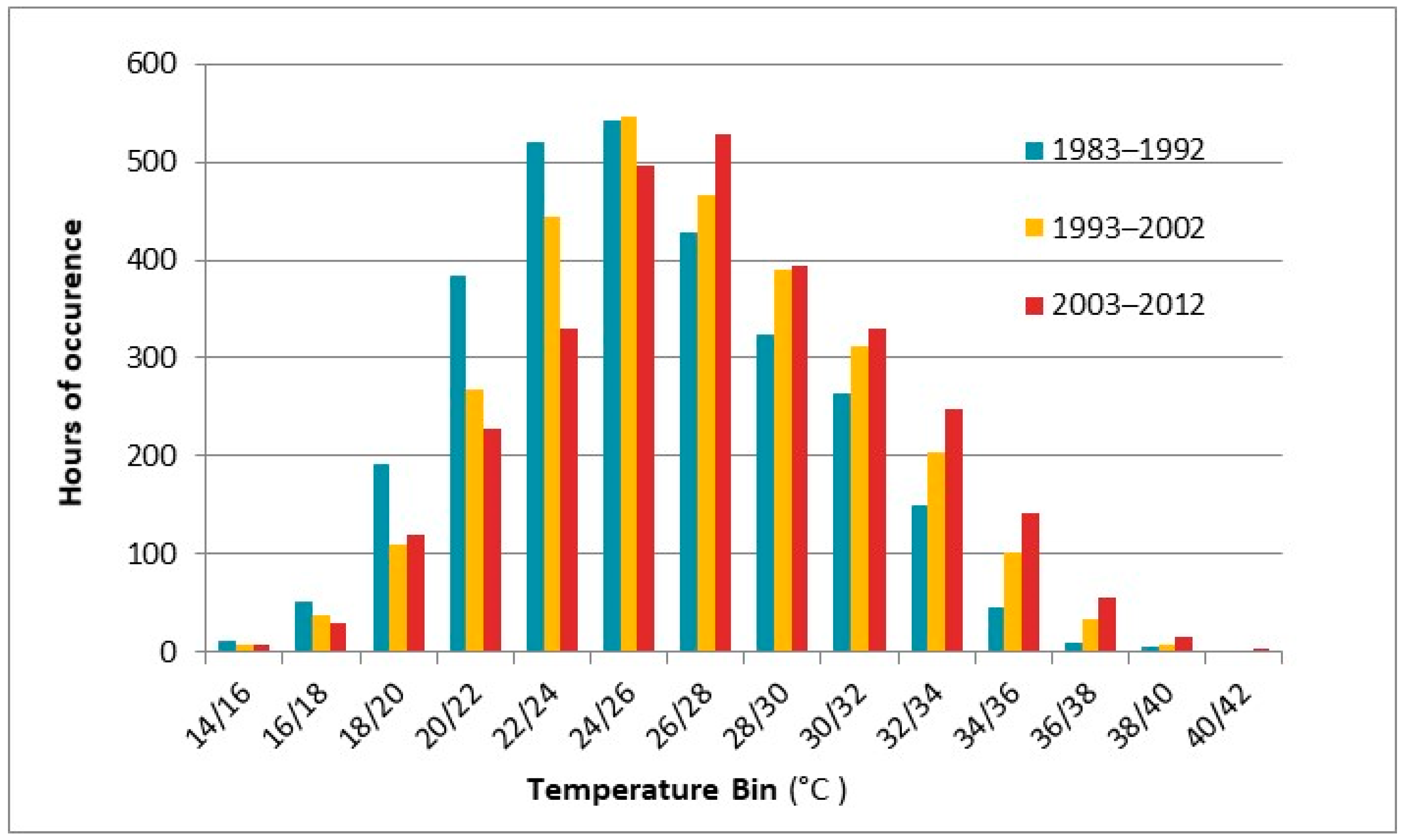
Annual or monthly aggregated values are useful for energy calculations only in the case that an average efficiency or performance of the HVAC equipment over the entire heating or cooling season is considered. The main problem with the mean annual and monthly temperature data and average efficiency ratings is that they do not account for equipment performance variations that occur hourly in response to weather changes. In the case of air source heat pumps, air cooled chillers and even condensing boilers, the efficiency varies with outdoor air temperature, thus disaggregated data are needed. Bin data, as mentioned in the previous section, are temperature data sorted into discrete groups (bins) of dry-bulb temperature conditions. Each bin contains the average number of hours of occurrence during a month, period or year of a particular range of dry-bulb temperature conditions along with the corresponding mean coincident wet-bulb temperature or humidity ratio. Thus, instead of using a single design condition for an entire month or year, heating, cooling or ventilation loads of a building can be calculated for each bin condition. In this work, binned distributions of outdoor air temperature for the 1983–1992, 1993–2002 and 2003–2012 time periods were calculated from hourly measurements. The frequency of occurrence (in h) of outdoor temperature in each equally sized temperature interval (bin) was calculated for each year separately, and then the results (the bin data) were averaged for the whole 10-year period. The cumulative results for the frequency of occurrence of 2 °C-wide temperature bins during the summer season (June to September), when buildings usually need cooling, during the winter season (November to April), when buildings need heating, and the transient months (May and October) when normally neither cooling nor heating is needed, but in buildings with forced ventilation systems the ventilation loads have to be considered, are presented in Figure 2, Figure 3 and Figure 4, respectively. The figures show the average number of hours that a particular temperature interval (bin) occurs in each season, for the three 10-year time periods separately. It is evident that the frequency distribution of temperature bins is shifting to the right, with a decrease in the low temperature bins and an increase in the high temperature bins every decade. It must be noted that some extreme temperature bins, with very low frequency, which represent very small percentages of hours during the heating season, the cooling season and the transient months (0.2%, 0.1% and 0.1%, respectively), were excluded from the results that appear in the figures.
During the cooling season (Figure 2), the frequency of occurrence (in h) of the temperature bins which are lower than 26 °C decreases progressively, (with some exceptions in some bins during the third decade), while it increases above this temperature threshold in every decade. The 24/26 °C interval is the most frequent temperature bin in the cooling season during the first 10-year period, 1983–1992 (Figure 2), with a frequency of 542 h of occurrence and a percentage frequency of 18.5%. The frequency of occurrence of this bin decreased to 497 h (17%) during the last 10-year period 2003–2012. In this last period, a higher temperature bin of 26/28 °C was the most frequent, with 529 h frequency of occurrence and a percentage frequency of 18.1%. Furthermore, the frequency of occurrence of the high temperature bins (>30/32 °C) almost doubled from 473 to 793 h, while peak temperature bins (>34/36 °C) more than tripled from 60 to 216 h.
During the heating season, the temperature threshold under which the frequency of temperature bins has decreased (and above which, respectively, it has increased) is 14 °C (Figure 3), a typical balanced temperature for very well-insulated buildings.
The corresponding most frequent temperature bin during the heating season is the 10/12 °C interval, with 758 h frequency of occurrence and a percentage frequency of 17.2%, but the frequency of this bin decreased to 698 h (16%) during the last 10-year period 2003–2012 and it was substituted by the 12/14 °C interval, with 780 h frequency of occurrence and a percentage frequency of 17.9%. On the other hand, a reduction from 976 to 757 h was observed in the occurrence of low temperature bins (<6/8 °C) while the occurrence of the temperature bins below 0/2 °C was reduced from 70 to 55 h. During the transient months, the same tendencies are observed (Figure 4).
The same trends, namely the increase of the frequency of hot days as well as the increase in number and duration of heat wave episodes (sequence of consecutive hot days), are observed by other researchers [35,37,42,43]. It is apparent that summers are becoming increasingly hotter, while the differences between the three decades during wintertime are less pronounced, although not insignificant. In general, the results confirm that for the city of Athens, the mean air temperature is constantly increasing and the climate is changing to relatively milder winters and harsher summers, which in turn leads to a decrease of energy consumption for heating purposes but also to a steep increase in energy consumption for cooling purposes [44,45,46].
The above analysis for the mean monthly air temperatures and dry-bulb air temperature bin data of Athens was also performed in a previous work [47]; nevertheless, the study did not make use of the revised version of NOA’s temperature data after the correction of detected inhomogeneity related to instruments change [34], as at the time they were not available. More specifically, two discontinuities were detected in the air-temperature time series at the meteorological station of the NOA. The first discontinuity reflects the instrumental change which took place in June 1995 and the second discontinuity (and most pronounced) reflects the application of a correction factor to the temperature values (in January 1997) after a calibration of the new thermometers. Before applying these changes, a significant number of temperature measurements during the second period of the present study (1993–2002) were incorrect. The present study makes use of the revised (homogenized) air temperature time series. Furthermore, in addition to the calculation of frequency (in hours) of outdoor air dry-bulb temperature, the corresponding values of the mean coincident humidity ratio and the mean coincident wet-bulb temperature (MCWB) at each temperature interval were calculated.
Namely, in this study, a humidity analysis was performed in addition to the temperature analysis in the three 10-year periods.

3.3. Estimation of the Mean Coincident Humidity Ratio

Hourly measurements of outdoor air dry-bulb temperature and relative humidity for the same period were used to calculate the humidity ratio of the air. The missing values in the examined period were about 1177 out of 262,992 observations recorded (0.4%) and the effect on the results was negligible.
Air humidity influences the energy consumption of an HVAC system, making the use of accurate data of paramount importance in the precise estimation of its energy consumption. Furthermore, when applying the modified bin method, the mean coincident absolute humidity values or the mean coincident wet-bulb temperature values corresponding to every temperature bin are necessary for the calculation of latent energy ventilation loads when evaluating HVAC systems.
Several constituents, including water vapor and other components, are found in atmospheric air (e.g., smoke, pollen, gaseous pollutants, etc.). The term “dry air” refers to air that is free of water vapor and other contaminants. Dry air and water vapor form moist air, which is a binary or two-component mixture. Humidity ratio of moist air is defined as the ratio of the total mass of water vapor to the mass of dry air contained in the mixture at the same temperature and pressure [48].
W = m w m a = 0.622 p w p a = 0.622 p w p p w ( kg H 2 O kg dry   air )
where:
p the atmospheric pressure, in Pa;
p a the partial pressure of dry air, in Pa;
p w the partial pressure of water vapor content in air, in Pa.
To calculate the humidity ratio W, the calculation of p and p w is required. The value of the atmospheric pressure depends on the altitude according to the following equation:
p = 101.325 ( 1 2.25577 × 10 5 Z ) 5.2559 ( kPa )
where Z is the altitude in m above sea level. The partial pressure of water vapor p w is related to the relative humidity φ as:
p w = p w s φ                 ( Pa )
where:
φ the relative humidity of moist air;
p w s the saturation pressure of water vapor at the air dry-bulb temperature corresponding to φ in Pa.
The saturation pressure can be determined as a function of dry-bulb temperature. For the temperature range from −100 °C to 0 °C, it is given by Equation (4), while for temperatures above 0 °C and up to 200 °C it is given by Equation (5) as follows:
ln p w s = 5674.54 T + 6.4 0.0097 T + 0.622 × 10 6 T 2 + 0.207 × 10 8 T 3 + 0.95 × 10 12 T 4 + 4.16 ln T
ln p w s = 5800.22 T + 1.39 0.0486 T + 0.417 × 10 4 T 2 + 0.144 × 10 7 T 3 + 6.545 ln T
where T is the absolute dry-bulb temperature in K.
The calculation procedure of the mean coincident humidity ratio for every temperature bin of 2 °C, in each month of the 30-year period, was the following:
For each month, a file with pairs of dry-bulb temperature and the corresponding relative humidity (t, φ) from the hourly records of NOA was created. In this file, the 24 h of the day were divided into six 4-h periods. For each pair of (t, φ) the humidity ratio was calculated using Equations (1)–(5). The values of dry-bulb temperature were categorized in bins of 2 °C and the average, maximum and minimum value of humidity ratio at each bin and 4-hour period of the day were calculated. Additionally, the average (mean coincident) humidity ratio and its range were calculated at each bin of 2 °C, for the whole day (24-h period). This procedure was followed for all months of each year of the three 10-year periods, namely 1983–1992, 1993–2002 and 2003–2012. Finally, the mean coincident humidity ratio values for each month and at each temperature bin were integrated for the whole 10-year period, and seasonal (winter, summer and transient) values were extracted. A comparison of the results between the three 10-year periods is shown in Figure 5, Figure 6 and Figure 7. As in the previous section, extreme temperature bins with very low frequency of occurrence were excluded from the results presented in figures.
In the cooling season (Figure 5), the humidity ratio has increased in almost all temperature bins (except for very high temperatures), when comparing the last 10-year period (2003–2012) with the first (1983–1992). The average increase of humidity ratio in the whole range of temperature bins is 0.0007 kg H2O/kg dry air (approximately 7.2%). During the heating season (Figure 6), it rises in all temperature bins above 10/12 °C with an average increase of 0.0002 kg H2O/kg dry air (2.1%). The temperature bin 24/26 °C is an exception, probably because the sample is very small. The same trends are observed during the transitional months (Figure 7) with an average increase of 0.0004 kg H2O/kg dry air (5.3%) between the two 10-year periods.
During the winter months, and particularly in January and February, there was an average rise in mean absolute humidity of 0.0003 (5.2%) and 0.0002 kg H2O/kg dry air (4.2%), respectively. During summer months the mean humidity ratio appears to have a stronger upward trend, with August showing a 0.0012 kg H2O/kg dry air increase (10%), while the average increase in July and September was 0.0008 and 0.0007 kg H2O/kg dry air, respectively (7.3% in both months). No noticeable changes were observed during the remaining summer or winter months. An upward trend of the maximum values of humidity ratio is also observed in all months, with its peak during the summer season.
From these comparisons it becomes apparent that there is an increase of the mean absolute humidity ratio in the outdoor air, with a gradual increase throughout the 30-year study period. This increase has an impact on the energy consumption required for the mechanical ventilation in buildings [49]. The energy consumption for dehumidification of outdoor air during the summer season is increased and for humidification during winter is decreased in HVAC systems.

3.4. Estimation of the Mean Coincident Wet-Bulb Temperature

The mean coincident wet-bulb (MCWB) temperatures were calculated with the use of Daikin Psychrometrics software [50]. First, the middle temperature value in each temperature bin was considered as the dry-bulb temperature. For every couple of dry-bulb temperature and coincident mean humidity ratio, the coincident wet-bulb temperature was estimated. The calculation procedure was as follows: the value of dry-bulb air temperature was kept constant, and the relative humidity was modified until the humidity ratio converged to the value of the mean coincident humidity ratio. The corresponding wet-bulb temperature was the MCWB temperature of the temperature bin. This method was applied for all temperature bins, in every month of the three 10-year periods.
The variations of the MCWB temperature follow the same trend with those of the mean coincident humidity ratio. In general, an increase of 0.6, 0.8 and 0.6 °C for July, August and September is evidenced between the first and the third 10-year period, while during the overall summer period it has increased by 3%. In the transient months, there was also a significant increase of the MCWB temperatures by 2.1%, while in the winter period there was a small rise of 1%, with the highest increase of 0.3 °C and 0.2 °C observed in January and February, respectively.
In similar works, observations and/or simulations indicate that the increase in air temperature is accompanied by an increase in the humidity ratio but also in changes in the maximum wet-bulb temperatures [51]. There is the danger that simultaneous occurrence of higher air temperature and humidity could make climate conditions in some areas intolerable to humans in the future [52].

3.5. Tables of Bin Data for Athens (NOA)

In the following Table 2, Table 3 and Table 4, the most recent (for the 2003–2012 period) bin data from the analysis that was performed, namely dry-bulb temperature, mean coincident absolute humidity and MCWB temperature for the city of Athens are presented.
Table 2 contains the data for the cooling period, Table 3 contains the data for the heating period and Table 4 the data for the transient months. The period of the day was divided into six 4-h shifts for a better part load energy analysis. The results are derived from monthly data [14]. These datasets can be used for the estimation of energy requirements and fuel consumption according to the bin and modified bin method [15,17], and may serve for updating the bin data of the Warmer zone of EN14825 [16].

4. Case Study

The energy demands for heating and cooling of an office building were estimated using the modified bin approach, in order to evaluate the influence of temperature data variations on building energy requirements [18,19]. Energy demands account for both sensible and latent loads, since the energy analysis presented refers to dry-bulb and wet-bulb temperature data, without taking into account the efficiency of the HVAC systems.
The structure used for this study is a typical university campus structure in Thessaloniki, which, for the purpose of this research, is assumed to be placed in the city of Athens. It has a rectangular shape and a sectional view of 16 × 49 m. The normal floor height is 3 m. The structure consists of nine levels with a ground floor with the main entrance, offices, a computer room, an assembly hall, a meeting room and a basement with different utilities. Figure 8 and Figure 9 depict the standard floor and ground floor, respectively.
The building has two main elevations, one to the north and one to the south. Without being overshadowed by any other structure, the apertures’ surfaces cover around 24% of the north, 32% of the south and 12.5% of the east and west perimeter areas of the building.
The thermal characteristics of the building elements are provided in Table 5 and Table 6.
The operating hours of the building are from 9:00 a.m. to 20:00 p.m., with an internal temperature of 20 °C in the heating season and 26 °C in the cooling season. Temperatures of 15 and 30 °C were assumed for the rest of the day. For the heating and cooling periods, the temperature of the stairwells and the entrance area was set at 15 and 30 °C in each case. Throughout the year, the ventilation rate was set at 1 and 0 ACH in operation and non-operation periods, respectively. The office building was simulated using the 3 decades (1983–1992, 1993–2002 and 2003–2012) temperature bin data of the city of Athens.

Resulting Impact of Climate Change on the Energy Demands for Heating and Cooling

It is obvious that there is a noticeable increase in the total energy requirements of the office building for cooling and dehumidification during the period from May to October, as highlighted in Figure 10 and in Table 5. There is an increase of approximately 10% per decade (11.4% in the second decade and 8.2% in the third), while overall cooling loads increased by 20.6%.
On the other hand, there is a noticeable decrease in the total energy requirements of the office building for heating and humidification during winter (from November to April), with a decrease of approximately 14.2% per decade (17.1% in the second decade and 11.4% in the third) and an overall heating load decrease of 26.5%, as evidenced in Figure 11 and in Table 5.
It should be pointed out that Figure 10 and Figure 11 present the sensible and latent energy requirement of the building, the performance coefficients of the primary equipment not being accounted for.
In particular, the increase in sensible loads accounts for 11.3% over the period considered, while in contrast, the increase in latent loads totals 62.6% in the three decades. The total increase in the energy requirements of the building for both heating and cooling from the first to the last decade is 14.5% (Table 7).
The trend of cooling loads is increasing in all summer months, especially in June, July and August, and is decreasing in all winter months (Figure 10). The decrease in the heating loads cannot offset the increase in cooling loads during the specified period, so overall energy requirements are increased. This is also reflected in the building’s specific energy requirements for heating and cooling.

5. Conclusions

In the present work, a 30-year long (1983–2012) time series of hourly outdoor air temperature and relative humidity records from the meteorological station of NOA in Athens, Greece was used to produce specific data for the application of bin methods. To that end, the outdoor air temperature and relative humidity hourly measurements were analyzed and the frequency of outdoor air dry-bulb temperature at intervals of 2 °C, as well as the corresponding mean coincident humidity ratio or wet-bulb temperature values, was calculated. The main goal was to provide an up-to-date bin data set for the city of Athens, based on recent records.
Some conclusions concerning the behavior of the calculated climate parameters during the selected time period and the impact of changes observed on local climate are discussed as well. From the results it is obvious that the annual average dry-bulb temperature increased by 1.12 °C over the 30-year period. The increase rate varies between summer and winter months, with an increase of up to 2.30 °C for August but only 0.29 °C in January. The temperature increase during the transient months is less pronounced. The same trend is evident in the distribution of temperature bins that were calculated as they shift to the right, namely in every decade a reduction of the low and an increase of the high temperature bins is observed. The most frequent temperature bin, during the heating season, was initially the 10/12 °C one but, during the period examined, it fell into second place and was replaced with the 12/14 °C bin (17.9% frequency). Likewise, for the cooling period, the 24/26 °C bin was replaced as the most frequent temperature bin by the 26/28 °C (18.1% frequency). Furthermore, the frequency of occurrence of the high temperature bins (>30/32 °C) almost doubled from 473 to 793 h, while peak temperature bins (>34/36 °C) more than tripled from 60 to 216 h.
The mean humidity ratio in the outdoor air also gradually increased throughout the study period, with an average increase of 7.2%. This increase is significant as it has an impact on the energy consumption required for the mechanical ventilation in buildings. The same trend is observed in the MCWB temperature as well, with an average increase of 2.1%. It is interesting to note here that analogous findings are reported in relevant studies. Nevertheless, it is beyond the scope of this study to investigate the causes behind the observed trends.
In conclusion, the total reduction in energy requirements for heating from the first (1983–1992) to the third decade (2003–2012) is 26.5%. Specifically, the decrease for sensible heating is 29.1%, because of the rising trend of ambient temperature, and the decrease for humidification is 10.2%, because of the rising trend of absolute humidity of the outdoor air. The corresponding total increase in energy requirements for cooling is 20.6%. More specifically, the increase for sensible cooling is 16.8%, and the increase for dehumidification is 90.1%. Thus, there is a particularly significant increase in the energy requirements for dehumidification, because of the increase in the absolute humidity of the outdoor air during the summer.
The total increase in the building’s annual energy requirements for air conditioning from the first to the third decade amounts to 14.5%.
The above results have important implications for power generation and supply systems, and changes in ambient air temperature will also have a significant impact on the performance of the cooling and heating equipment, if heat pumps are used, and the ability to use outside air for “free cooling”.
From the above it is clear that these data can be used for detailed estimation of the energy requirements in the built environment for practitioners to achieve an easy and qualitative energy assessment of an HVAC system. Accurate estimation of heating and cooling energy needs is the key to successful design of HVAC systems which leads to reduced operational cost. Today, HVAC energy analysis simulation tools supported by recent climate data which include the effects of climate change are necessary to accurately predict HVAC energy performance and to develop and preserve indoor comfort conditions in buildings.

Author Contributions

Conceptualization, K.T.P. and G.M.; methodology, K.T.P.; software, D.K., K.K.; validation, D.K., K.K.; resources, D.F.; data curation, K.T.P.; writing—original draft preparation, G.M.; writing—review and editing, G.M., K.T.P., D.F. All authors have read and agreed to the published version of the manuscript.

Funding

This research received no external funding.

Conflicts of Interest

The authors declare no conflict of interest.

References

  1. IPCC. Climate Change 2014: Synthesis Report. Contribution of Working Groups I, II and III to the Fifth Assessment Report of the Intergovernmental Panel on Climate Change; Pachauri, R.K., Meyer, L.A., Eds.; IPCC: Geneva, Switzerland, 2014; p. 151. [Google Scholar]
  2. Ogunbode, C.A.; Demski, C.; Capstick, S.B.; Sposato, R.G. Attribution matters: Revisiting the link between extreme weather experience and climate change mitigation responses. Glob. Environ. Change 2019, 54, 31–39. [Google Scholar] [CrossRef]
  3. NOAA (2018) National Centers for Environmental Information, Climate at a Glance: Global Time Series. Available online: https://www.ncdc.noaa.gov/cag/ (accessed on 9 September 2020).
  4. Global Climate Report—Annual 2018. Available online: https://www.ncdc.noaa.gov/sotc/global/201813 (accessed on 24 September 2020).
  5. Perkins-Kirkpatrick, S.E.; Gibson, P.B. Changes in regional heatwave characteristics as a function of increasing global temperature. Sci. Rep. 2017, 7, 1–12. [Google Scholar] [CrossRef]
  6. Diffenbaugh, N.S.; Pal, J.S.; Giorgi, F.; Gao, X. Heat stress intensification in the Mediterranean climate change hotspot. Geophys. Res. Lett. 2007, 34, L11706. [Google Scholar] [CrossRef] [Green Version]
  7. Pérez-Andreu, V.; Aparicio-Fernández, C.; Martínez-Ibernón, A.; Vivancos, J.L. Impact of climate change on heating and cooling energy demand in a residential building in a Mediterranean climate. Energy 2018, 165, 63–74. [Google Scholar] [CrossRef]
  8. Energy Efficient Buildings. Available online: https://ec.europa.eu/energy/en/topics/energy-efficiency/buildings (accessed on 11 August 2019).
  9. Gildiz, I. Review of climate issues: A forcing function perspective in agricultural and energy innovation. Int. J. Energy Res. 2019, 43, 2200–2215. [Google Scholar]
  10. Martinopoulos, G.; Papakostas, K.T.; Papadopoulos, A.M. A comparative review of heating systems in EU countries, based on efficiency and fuel cost. Renew. Sustain. Energy Rev. 2018, 90, 687–699. [Google Scholar] [CrossRef]
  11. Martinopoulos, G.; Serasidou, A.; Antoniadou, P.; Papadopoulos, A.M. Building integrated shading and building applied photovoltaic system assessment in the energy performance and thermal comfort of office buildings. Sustainability 2018, 10, 4670. [Google Scholar] [CrossRef] [Green Version]
  12. Uner, M.; Ileri, A. Typical weather data of main Turkish cities for energy applications. Int. J. Energy Res. 2000, 24, 727–748. [Google Scholar] [CrossRef]
  13. National Observatory of Athens. Climatological Bulletin (1983–2012); Institute of Meteorology and Physics of the Atmospheric Environment: Athens, Greece, 2015. [Google Scholar]
  14. Kyrou, D. Statistical Analysis of Hourly Ambient Air Dry-Bulb Temperature and Relative Humidity Observations for the Period 1983–2012 in Athens (NOA)—Elaboration of Data for HVAC Energy Analysis Methods; Mechanical Engineering Deptartment, Aristotle University of Thessaloniki: Thessaloniki, Greece, March 2018. [Google Scholar]
  15. ASHRAE. Handbook of Fundamentals; American Society of Heating Refrigerating and Air-Conditioning Engineers, Inc.: Atlanta, GA, USA, 1983. [Google Scholar]
  16. European Standard EN 14825:2018. Air Conditioners, Liquid Chilling Packages and Heat Pumps, with Electrically Driven Compressors, for Space Heating and Cooling–Testing and Rating at Part Load Conditions and Calculation of Seasonal Performance; European Committee for Standardization: Brussels, Belgium, 2018. [Google Scholar]
  17. Knebel, D.E. Simplified Energy Analysis Using the Modified Bin Method; American Society of Heating, Refrigerating and Air-Conditioning Engineers, Inc.: Atlanta, GA, USA, 1983. [Google Scholar]
  18. European Standard EN ISO 52016-1:2017. Energy Performance of Buildings—Energy Needs for Heating and Cooling, Internal Temperatures and Sensible and Latent Heat Loads—Part 1: Calculation Procedures; European Committee for Standardization: Brussels, Belgium, 2017. [Google Scholar]
  19. Papakostas, K.T. Technical note Bin weather data of Athens, Greece. Renew. Energy 1999, 17, 265–275. [Google Scholar] [CrossRef]
  20. ASHRAE. Handbook Fundamentals; American Society of Heating, Refrigerating and Air Conditioning Engineers, Inc.: Atlanta, GA, USA, 2013. [Google Scholar]
  21. Moazami, A.; Nik, V.M.; Carlucci, S.; Geving, S. Impacts of future weather data typology on building energy performance–Investigating long-term patterns of climate change and extreme weather conditions. Appl. Energy 2019, 238, 696–720. [Google Scholar] [CrossRef]
  22. Martinopoulos, G.; Alexandru, A.; Papakostas, K.T. Mapping temperature variation and degree-days in metropolitan areas with publicly available sensors. Urban Clim. 2019, 28, 100464. [Google Scholar] [CrossRef]
  23. Wang, Z.; Ding, Y.; Geng, G.; Zhu, N. Analysis of energy efficiency retrofit schemes for heating, ventilating and air-conditioning systems in existing office buildings based on the modified bin method. Energy Convers. Manag. 2014, 77, 233–242. [Google Scholar] [CrossRef]
  24. Coakley, D.; Raftery, P.; Keane, M. A review of methods to match building energy simulation models to measured data. Renew. Sustain. Energy Rev. 2014, 37, 123–141. [Google Scholar] [CrossRef] [Green Version]
  25. Papakostas, K.T.; Pitsavou, F. Condensing Boilers and Variable Speed Pumps as a Refurbishment Option for Heating Systems in Residential Buildings—Energy and Economic Evaluation. IOP Conf. Ser. Mater. Sci. Eng. 2018, 444, 082001. [Google Scholar] [CrossRef]
  26. Kneifel, J.; O’Rear, E.; Webb, D.; O’Fallon, C. An exploration of the relationship between improvements in energy efficiency and life-cycle energy and carbon emissions using the BIRDS low-energy residential database. Energy Build. 2018, 160, 19–33. [Google Scholar] [CrossRef] [PubMed]
  27. Said, S.A.M.; Habib, M.A.; Iqbal, M.O. Database for building energy prediction in Saudi Arabia. Energy Convers. Manag. 2003, 44, 191–201. [Google Scholar] [CrossRef]
  28. Ozyurt, O.; Bakirci, K.; Erdogan, S.; Yilmaz, M. Bin Weather Data for the Provinces of the Eastern Anatolia in Turkey. Renew. Energy 2009, 34, 1319–1332. [Google Scholar] [CrossRef]
  29. Pusat, S. A simple approach to estimate ambient temperature bin data. Energy Effic. 2019, 12, 1053–1064. [Google Scholar] [CrossRef]
  30. Idchabani, R. Bin weather data for five climatic zones of Morocco. Int. J. Ambient Energy 2018, 41, 954–961. [Google Scholar] [CrossRef]
  31. Papakostas, K.; Bentoulis, A.; Bakas, V.; Kyriakis, N. Estimation of Ambient Temperature bin Data from Monthly Average Temperatures and Solar Clearness Index. Validation of the Methodology in Two Greek Cities. Renew. Energy 2007, 32, 991–1005. [Google Scholar] [CrossRef]
  32. Papakostas, K.; Tsilingiridis, G.; Kyriakis, N. Bin Weather Data for 38 Greek Cities. Appl. Energy 2008, 85, 1015–1025. [Google Scholar] [CrossRef]
  33. Zhang, P.; Jin, Z.; Guoqiang, Z.; Yezheng, W. Generation of Ambient Temperature Bin Data of 26 Cities in China. Energy Convers. Manag. 2009, 50, 543–553. [Google Scholar]
  34. Founda, D.; Kambezidis, H.D.; Petrakis, M.; Zanis, P.; Zerefos, C. A correction of the recent air-temperature record at the historical meteorological station of the National Observatory of Athens (NOA) due to instrument change. Theor. Appl. Climatol. 2009, 97, 385–389. [Google Scholar] [CrossRef]
  35. Founda, D. Evolution of the air temperature in Athens and evidence of climatic change: A review. Adv. Build. Energy Res. 2011, 5, 7–41. [Google Scholar] [CrossRef]
  36. Founda, D.; Pierros, F.; Katavoutas, G.; Keramitsoglou, I. Observed trends in thermal stress at European cities with different background climates. Atmosphere 2019, 10, 436. [Google Scholar] [CrossRef] [Green Version]
  37. Founda, D.; Papadopoulos, K.H.; Petrakis, M.; Giannakopoulos, C.; Good, P. Analysis of mean, maximum, and minimum temperature in Athens from 1897 to 2001 with emphasis on the last decade: Trends, warm events, and cold events. Glob. Planet. Chang. 2004, 44, 27–38. [Google Scholar] [CrossRef]
  38. Founda, D.; Pierros, F.; Petrakis, M.; Zerefos, C. Interdecadal variations and trends of the Urban Heat Island in Athens (Greece) and its response to heat waves. Atmos. Res. 2015, 161, 1–13. [Google Scholar] [CrossRef]
  39. Founda, D.; Giannakopoulos, C. The exceptionally hot summer of 2007 in Athens, Greece—A typical summer in the future climate? Glob. Planet. Change 2009, 67, 227–236. [Google Scholar] [CrossRef]
  40. Founda, D.; Santamouris, M. Synergies between Urban Heat Island and Heat Waves in Athens (Greece), during an extremely hot summer (2012). Sci. Rep. 2017, 7, 10973. [Google Scholar] [CrossRef] [PubMed] [Green Version]
  41. Kostopoulou, E.; Giannakopoulos, C.; Hatzaki, M.; Karali, A.; Hadjinicolaou, P.; Lelieveld, J.; Lange, M.A. Spatio-temporal patterns of recent and future climate extremes in the eastern Mediterranean and Middle East region. Nat. Hazards Earth Syst. Sci. 2014, 14, 1565–1577. [Google Scholar] [CrossRef] [Green Version]
  42. Slini, T.; Papakostas, K.T. 30 Years Air Temperature Data Analysis in Athens and Thessaloniki, Greece. In Energy, Transportation and Global Warming; Springer: Cham, Switzerland, 2016; pp. 21–33. [Google Scholar]
  43. Nastos, P.T.; Matzarakis, A.P. Variability of tropical days over Greece within the second half of the twentieth century. Theor. Appl. Climatol. 2008, 93, 75–89. [Google Scholar] [CrossRef]
  44. Cartalis, C.; Synodinou, A.; Proedrou, M.; Tsangrassoulis, A.; Santamouris, M. Modifications in energy demand in urban areas as a result of climate changes: An assessment for the southeast Mediterranean region. Energy Convers. Manag. 2001, 42, 1647–1656. [Google Scholar] [CrossRef]
  45. Papakostas, K.; Mavromatis, T.; Kyriakis, N. Impact of the ambient temperature rise on the energy consumption for heating and cooling in residential buildings of Greece. Renew. Energy 2010, 35, 1376–1379. [Google Scholar] [CrossRef]
  46. Papakostas, K.T.; Michopoulos, A.; Mavromatis, T.; Kyriakis, N. Changes of temperature data for energy studies over time and their impact on energy consumption and CO2 emissions. The case of Athens and Thessaloniki–Greece. Int. J. Energy Environ. 2013, 4, 59–72. [Google Scholar]
  47. Papakostas, K.; Zagana-Papavasileiou, P.; Mavromatis, T. Analysis of 3 Decades Temperature Data for Athens and Thessaloniki, Greece: Impact of Temperature Changes on Energy Consumption for Heating and Cooling of Buildings. In Proceedings of the International Conference ADAPTtoCLIMATE, Nicosia, Cyprus, 27–28 March 2014. [Google Scholar]
  48. ASHRAE. Psychrometrics-Theory and Praxis; American Society of Heating, Refrigerating, and Air Conditioning Engineers, Inc.: Atlanta, GA, USA, 1996. [Google Scholar]
  49. Papakostas, K.T.; Slini, T. Effects of Climate Change on the Energy Required for the Treatment of Ventilation Fresh Air in HVAC Systems—The Case of Athens and Thessaloniki. Procedia Environ. Sci. 2017, 38, 852–859. [Google Scholar] [CrossRef]
  50. Daikin Psychometrics Diagram Viewer. Available online: https://www.daikin-ce.com/en_us/customers/software-downloads/daikin-psychometrics-diagram-viewer.html (accessed on 10 September 2017).
  51. Li, J.; Chen, Y.D.; Gan, T.Y.; Lau, N.C. Elevated increases in human-perceived temperature under climate warming. Nat. Clim. Chang. 2018, 8, 43–47. [Google Scholar] [CrossRef]
  52. Schär, C. Climate extremes: The worst heat waves to come. Nat. Clim. Chang. 2016, 6, 128–129. [Google Scholar] [CrossRef]
Figure 1. Average values of mean monthly air temperatures in Athens (NOA) for the three decades 1983–1992, 1993–2002 and 2003–2012.
Energies 14 03501 g001
Figure 2. Temperature bin hours of occurrence in 2 °C intervals. Athens (NOA) (cooling season—June to September).
Energies 14 03501 g002
Figure 3. Temperature bin hours of occurrence in 2 °C intervals. Athens (NOA) (heating season—November to April).
Energies 14 03501 g003
Figure 4. Temperature bin hours of occurrence in 2 °C intervals. Athens (NOA) (transitional months—October and May).
Energies 14 03501 g004
Figure 5. Mean coincident humidity ratio, in 2 °C temperature intervals, Athens (NOA) (cooling season—June to September).
Energies 14 03501 g005
Figure 6. Mean coincident humidity ratio, in 2 °C temperature intervals, Athens (NOA) (heating season—November to April).
Energies 14 03501 g006
Figure 7. Mean coincident humidity ratio, in 2 °C temperature intervals, Athens (NOA) (transitional months—October and May).
Energies 14 03501 g007
Figure 8. Plan view of the building’s typical floor.
Energies 14 03501 g008
Figure 9. Plan view of the building’s ground floor.
Energies 14 03501 g009
Figure 10. Total (sensible and latent) monthly energy requirements for cooling.
Energies 14 03501 g010
Figure 11. Total (sensible and latent) monthly energy requirements for heating.
Energies 14 03501 g011
Table 1. Mean monthly and average annual air temperatures of the three time periods, Athens.
10-YEAR PERIODJANFEBMARAPRMAYJUNJULAUGSEPOCTNOVDECAVER
1983–19929.469.3511.4715.7819.9524.4427.1426.7723.5018.3213.8810.1317.52
1993–20029.5110.2311.7815.5421.1026.0528.4527.9623.9019.1614.3610.9618.25
2003–20129.759.4512.5516.0721.3126.3529.2029.0724.1019.3414.8511.5518.63
Table 2. Bin data for Athens (NOA). Cooling season (June to September)—Period 2003–2012.
Temperature Interval (Bin) (°C)Time Period of Day/Hours ObservedMean Coincident Humidity Ratio (kg H2O/kg Dry Air)MCWB (°C)
01:00–04:0005:00–09:0009:00–12:0012:00–16:0016:00–20:0020:00–24:00Total h–Served
12.0/14.000000000.007611.3
14.0/16.033001180.008412.9
16.0/18.010121025300.008513.8
18.0/20.04444516191190.011116.8
20.0/22.0676513519582270.010717.2
22.0/24.08988291245673300.011218.3
24.0/26.01361224630591044970.011519.1
26.0/28.099956749831365290.011619.8
28.0/30.034458856100713940.011520.4
30.0/32.06121079289233290.011621.0
32.0/34.011791105342480.011521.5
34.0/36.00037822201410.011622.1
36.0/38.000133580560.011622.7
38.0/40.00031110150.010922.7
40.0/42.000130040.011623.7
42.0/44.000010010.008121.9
Table 3. Bin data for Athens (NOA). Heating season (November to April)—Period 2003–2012.
Temperature Interval (Bin) (°C)Time Period of Day/Hours—ObservedMean Coincident Humidity Ratio (kg H2O/kg Dry Air)MCWB (°C)
01:00–04:0005:00–09:0009:00–12:0012:00–16:0016:00–20:0020:00–24:00Total h–Served
−6.0/−4.001100020.0025-5.0
−4.0/−2.010001130.0026-3.6
−2.0/0.0231112100.0032-1.5
0.0/2.011115246390.0030-0.5
2.0/4.0242913612221060.00331.0
4.0/6.04752321732372170.00372.7
6.0/8.07986583749703790.00444.7
8.0/10.0114129815074945420.00526.8
10.0/12.0149144102711001326980.00618.7
12.0/14.0146133121951351507800.006910.5
14.0/16.097831141231391236790.007512.0
16.0/18.038379012592614430.007913.2
18.0/20.01412579652212520.008314.3
20.0/22.03334612561320.008415.1
22.0/24.000123181520.009316.6
24.0/26.00031010140.008716.8
26.0/28.000120030.008717.5
28.0/30.000000000.005815.7
Table 4. Bin data for Athens (NOA). Transitional months (May and October)—Period 2003–2012.
Temperature Interval (Bin) (°C)Time Period of Day/Hours ObservedMean Coincident Humidity Ratio (kg H2O/kg Dry Air)MCWB (°C)
01:00–04:0005:00–09:0009:00–12:0012:00–16:0016:00–20:0020:00–24:00Total h–Served
6.0/8.000000000.00465.1
8.0/10.022100050.00567.3
10.0/12.0571134210.00618.8
12.0/14.0151553612560.006710.4
14.0/16.0384010512211260.007712.2
16.0/18.06464211126482320.008814.0
18.0/20.06966382345703110.009515.4
20.0/22.04135453253582640.009916.5
22.0/24.01213484454271980.010117.3
24.0/26.02439513271350.010118.0
26.0/28.0012440121780.010218.7
28.0/30.000112460410.009919.1
30.0/32.0004920150.010019.8
32.0/34.000130040.009620.1
34.0/36.000010010.012122.4
36.0/38.000000000.011822.8
Table 5. Thermal properties of structural elements.
Building ElementHeat Transfer Coefficient (W/m2K)
Exterior wall with thermal insulation0.6
Flat roof0.454
Windowsill2.25
Concrete pillar/beam2.25
Floor0.566
Table 6. Heat transfer coefficients U (W/m2K) and shading coefficients SC of windows.
Window Types (Layer/Frame)Room/SpaceU (W/m2K) (Summer)U (W/m2K) (Winter)Shading CoEfficient SC
Double, metalFloors’ offices/corridors3.330.85
Single, metalGround floor offices/rooms4.64.71
Single, metalStaircases66.41
Table 7. Latent and sensible loads for the 1983–2013 period.
Time PeriodCooling LoadsHeating Loads
SensibleLatentTotal (kWh)SensibleLatentTotal (kWh)
1983–199294.8%5.2%413,00986.7%13.3%60,804
1993–200295.0%5.0%460,18487.0%13.8%50,403
2003–201291.8%8.2%497,96383.7%16.3%44,665
Publisher’s Note: MDPI stays neutral with regard to jurisdictional claims in published maps and institutional affiliations.

