A Methodology for Robust Load Reduction in Wind Turbine Blades Using Flow Control Devices

Abstract

Decades of wind turbine research, development and installation have demonstrated reductions in levelized cost of energy (LCOE) resulting from turbines with larger rotor diameters and increased hub heights. Further reductions in LCOE by up-scaling turbine size can be challenged by practical limitations such as the square-cube law: where the power scales with the square of the blade length and the added mass scales with the volume (the cube). Active blade load control can disrupt this trend, allowing longer blades with less mass. This paper presents the details of the development of a robust load control system to reduce blade fatigue loads. The control system, which we coined sectional lift control or SLC, uses a lift actuator model to emulate an active flow control device. The main contributions of this paper are: (1) Methodology for SLC design to reduce dynamic blade root moments in a neighborhood of the rotor angular frequency (1P). (2) Analysis and numerical evidence supporting the use of a single robust SLC for all wind speeds, without the need for scheduling on wind speed or readily available measurements such as collective pitch or generator angular speed. (3) Intuition and numerical evidence to demonstrate that the SLC and the turbine controller do not interact. (4) Evaluation of the SLC using a full suite of fatigue and turbine performance metrics.

1. Introduction

With advancements in wind turbine technologies, turbine sizes have increased significantly in the last few decades, and large rotors are becoming increasingly important for utility-scale wind power. This is because larger turbines exhibit relatively lower electricity generation costs due to the higher wind speeds and the larger swept areas. However, larger turbines suffer from more fatigue damage due to unsteady aerodynamic loads [1]. Mitigating these loads using conventional turbine design approaches makes them heavy and expensive.

A well-known method to reduce the fatigue loads on the turbine blades is individual pitch control (IPC) [2,3,4]. IPC generates pitch angle commands for the pitch actuator on each blade, based on the feedback of dynamic loads. IPC can be implemented using different axes transformations like Clarke transformation [5] and multi-blade coordinate transformation [6,7,8] (also known as Coleman transformation). These transformations perform projections onto a set of orthogonal axes for both the measured loads and pitch commands. IPC can also be designed such that individual blades have separate control loops that utilize the local load on the particular blade to generate independent pitch commands for each blade without communicating with each other [9,10]. This approach is known as single-blade control or individual (i.e., independent) blade control. Reference [11] showed that the two transformation-based approaches and individual blade control are fundamentally similar and result in similar load reduction. IPC can be implemented in a feedback-feedforward framework where the feedback control loop utilizes sensed load while feedforward control utilizes wind estimates to improve disturbance rejection [12,13]. The wind estimate can be provided by a Kalman filter or LiDAR, with the latter providing true feedforward control. Load reduction using IPC has also been explored with additional local flow sensors [14], using advance control design techniques like model predictive control [15,16] and to reduce both fatigue and ultimate loads [17].

Although IPC results in a reduction in loads, its use may lead to excessive wear of the pitch actuators [18]. This concern grows with turbine size due to longer and potentially heavier blades. Thus, on-blade, active load control devices offer an attractive alternative to increase rotor size while disrupting the growth of turbine capital costs. An active on-blade load control system could mitigate loads before they develop, which would allow turbines to be built with less material and at a lower cost. Alternatively, blade lengths can be extended for constant load envelope, leading to increased annual energy production (AEP) and reduced levelized cost of energy (LCOE). Active load control solutions have been extensively researched, including trailing edge flaps, microtabs, shape changing blades, and others [18,19]. Among these actuators, trailing edge flaps have been studied the most [20,21] and compared with IPC [22]. They have also been tested on a full-scale wind turbine [23]. However, some of the challenges with these approaches lie in their mechanical complexity, costs, and maintainability in real-world conditions.

In this research, we focus on the development of a new load control system based on a Dielectric Barrier Discharge (DBD) plasma actuator (Figure 1) due to Arctura [24], which is mechanically simple with no moving parts [24]. We are part of a team [25] developing a controllable Gurney flap (GF) for wind turbine blades using DBD plasma actuators. Our team seeks to integrate actuator development, control systems and design methods to determine the greatest potential impact of the technology on reducing LCOE through a combination of modeling, design optimization and testing (wind tunnel and field rotor demonstration).

In the current paper, we describe a specific methodology for control system design to support the development of wind turbines with controllable GFs. This methodology is comprised of the following building blocks:

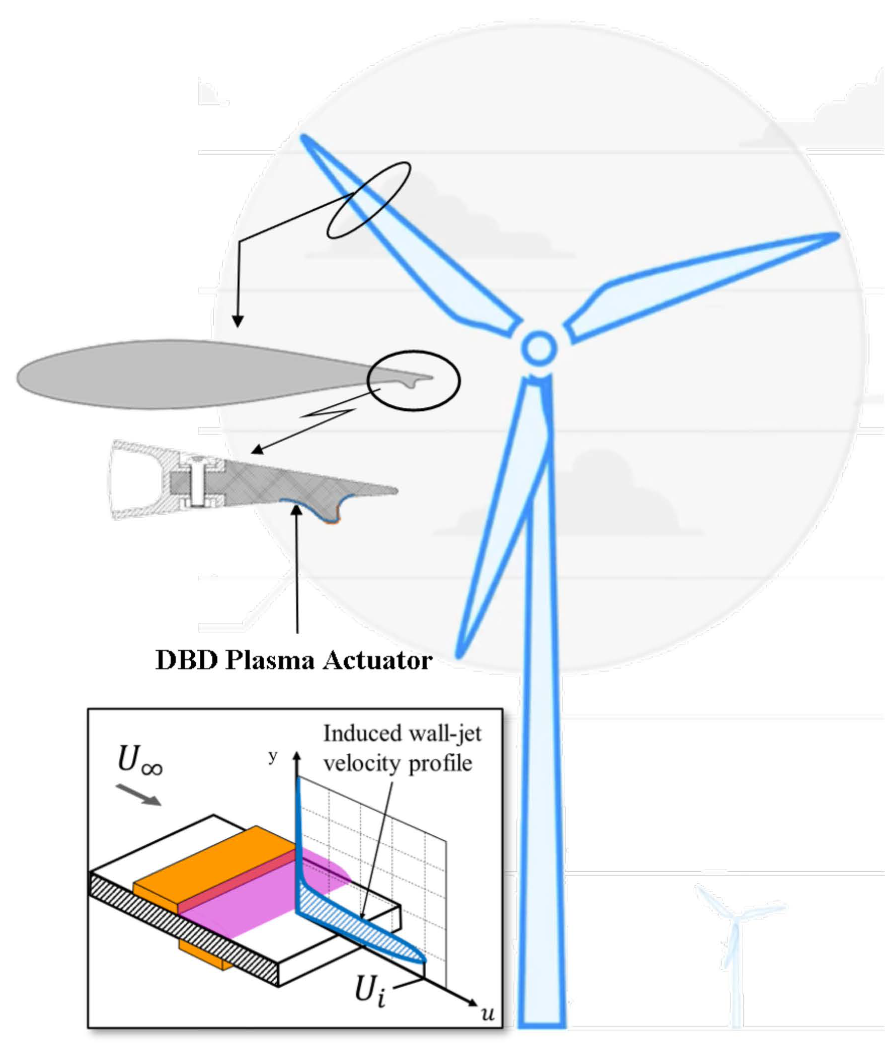
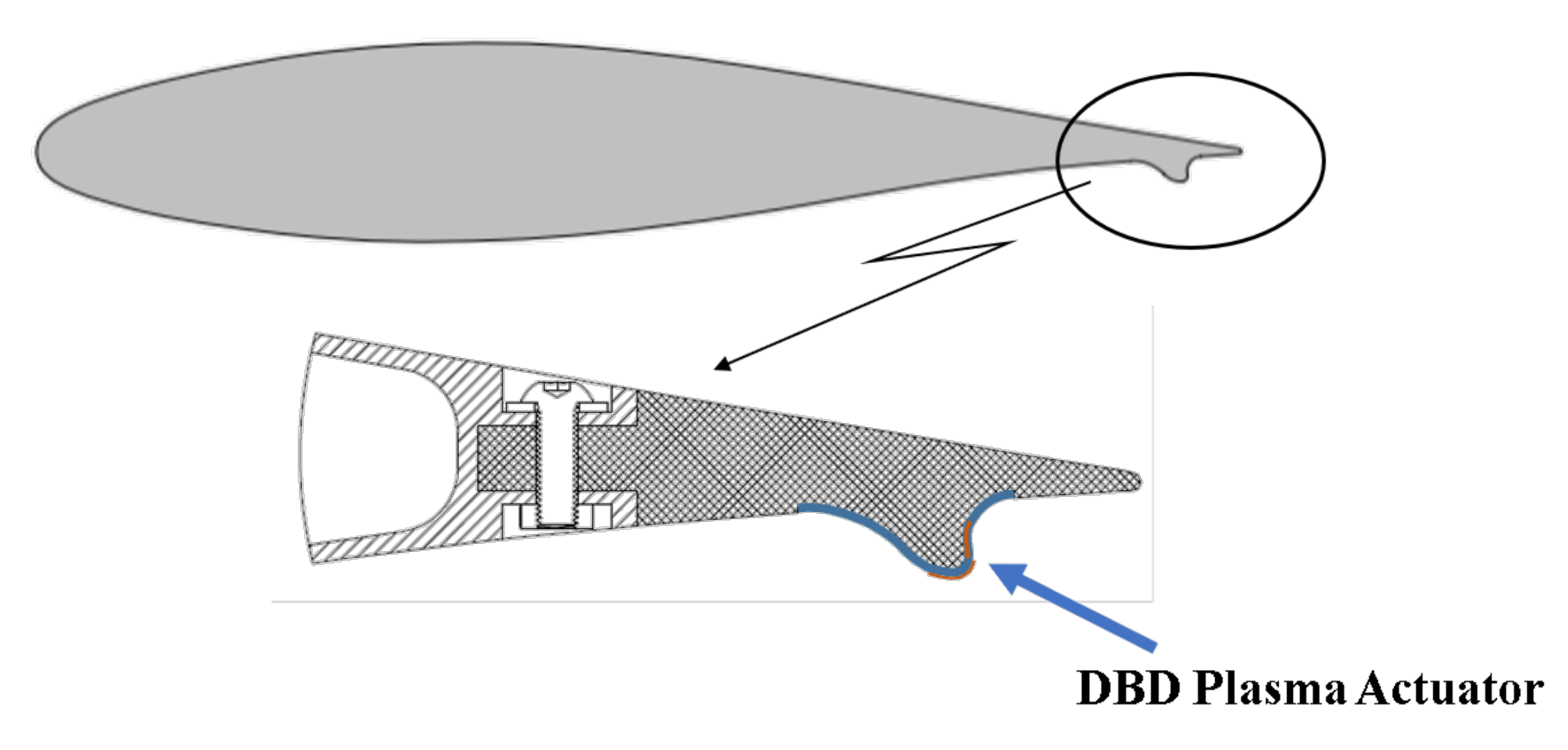
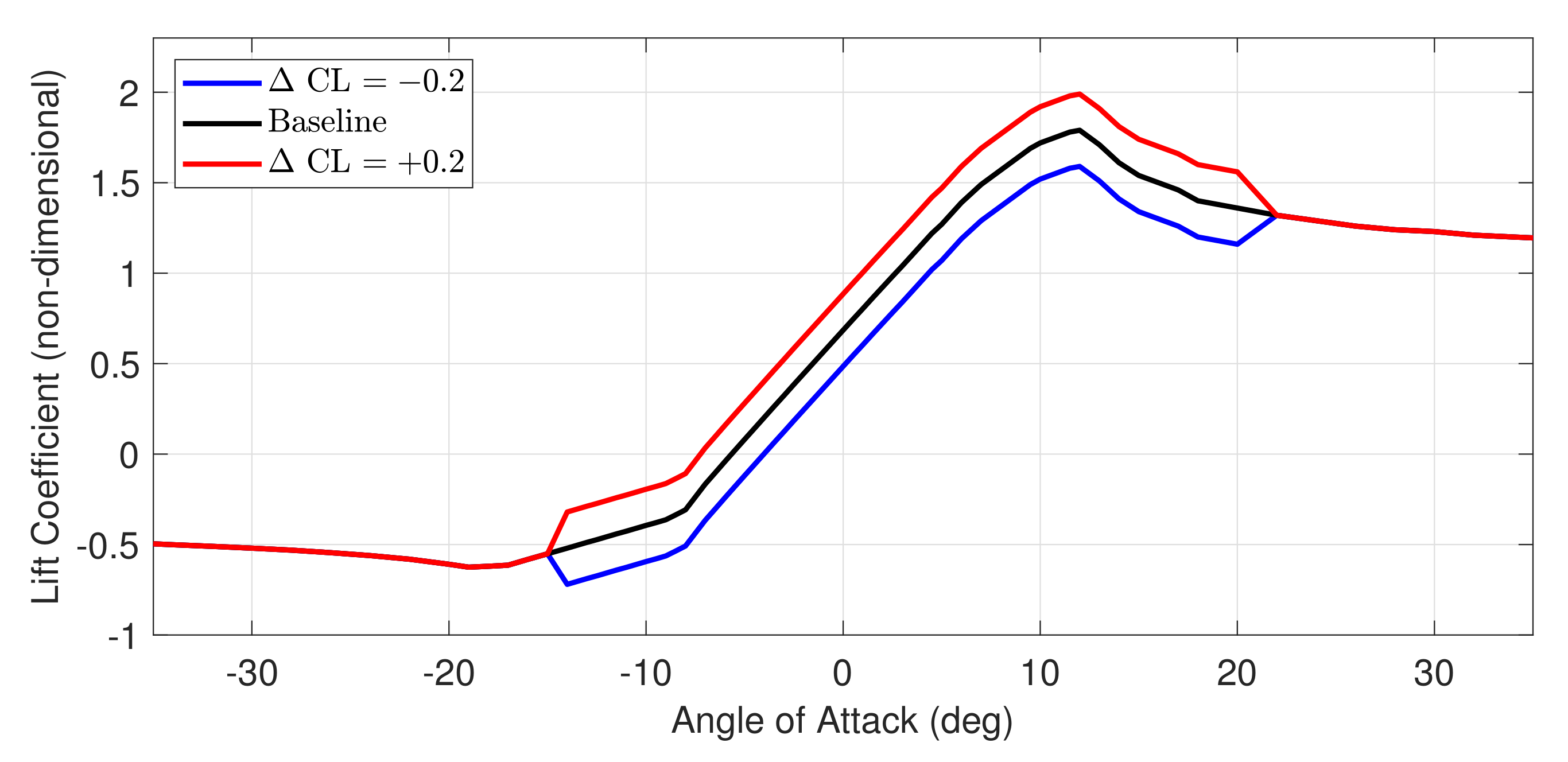
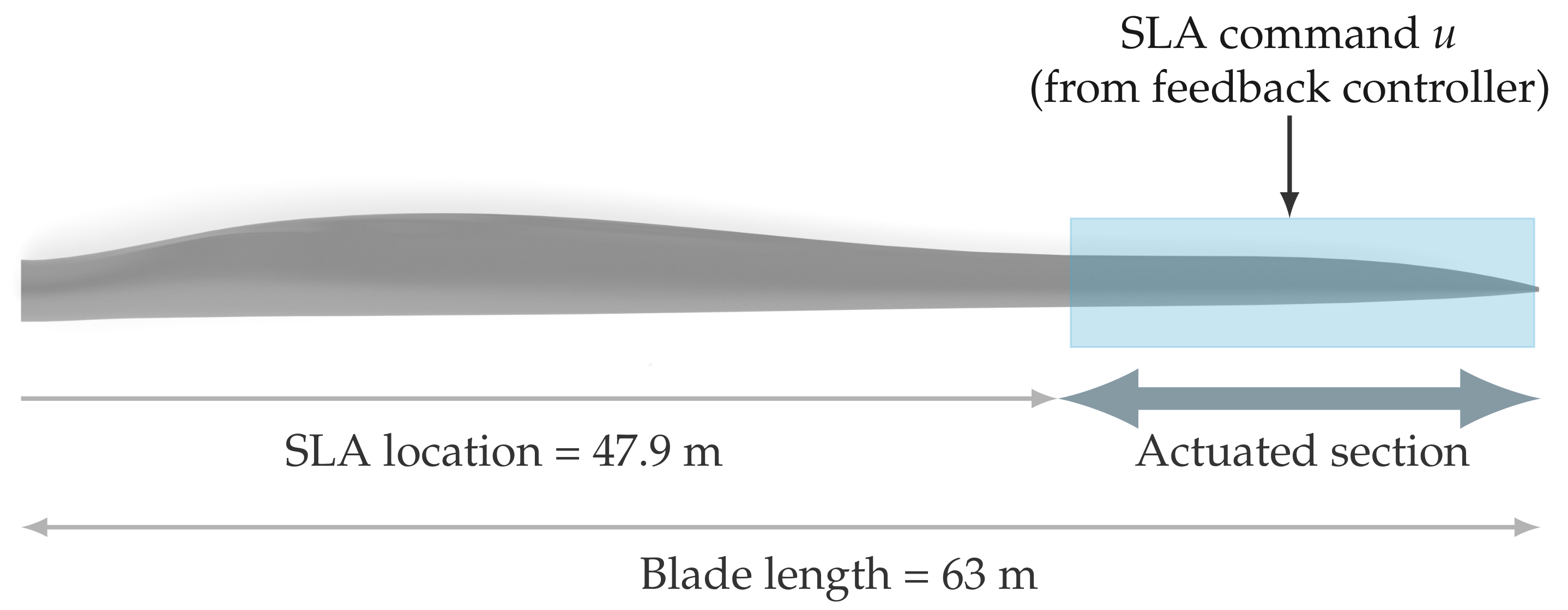
• Modeling the effect of the DBD plasma actuator as a dynamic change in local lift coefficient at the location where the actuator is placed. We refer to this modeling assumption as sectional lift actuation (SLA).
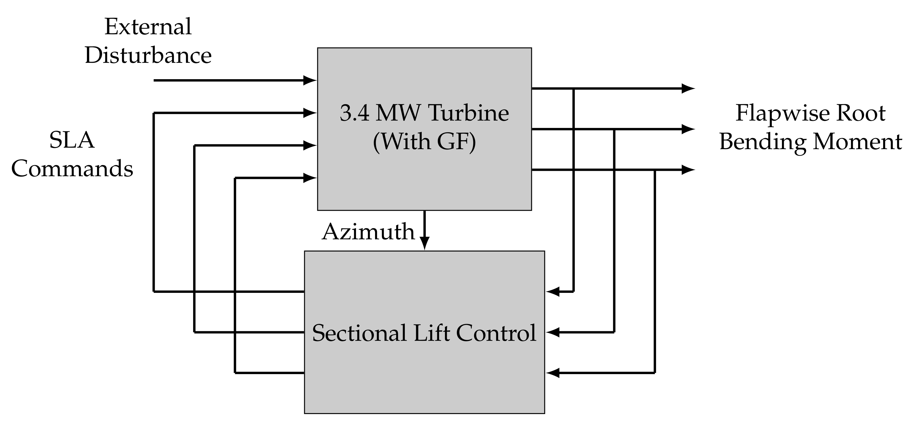
• A control system architecture based on the well-known multi-blade coordinate transformation [6] to reduce dynamic loads of the blade-root flapwise bending moments. This control system, which drives the sectional lift actuators, is coined sectional lift control (SLC).
• A feedback control algorithm designed to achieve load reduction and robustness to both (a) parametric uncertainty in the design model and (b) unmodeled dynamics.

This paper has two major contributions. Firstly, the methodology for design of the control system algorithm (Section 4). This methodology uses system identification tools to determine a dynamic model appropriate for controller design, and then a method for robust control synthesis in the frequency domain to obtain the control algorithm. Secondly, the application of this methodology to the design of a sectional lift controller for a 3.4 MW wind turbine. This 3.4 MW turbine is based on the IEA 3.4 MW reference turbine [26] but features a re-designed rotor and a re-tuned baseline turbine controller that accounts for the presence of the Gurney flap [27]. The designed SLC achieves reductions in blade-root flapwise damage equivalent loads ranging from 4% to 8% in below-rated wind speeds, to 8% to 12% in above-rated wind speeds with no adverse effect on other wind turbine loads, power production and pitch actuator activity (Section 5). The resulting SLC also reduces blade-tip deflections. We demonstrate, by example, that a single robust SLC designed for an above-rated wind speed suffices to reduce loads for all wind conditions. We give evidence that this property likely generalizes to other turbines with similar dynamic behavior.

This paper is organized as follows. Section 2 provides the specifications of the 3.4 MW turbine on which this study is conducted. The model of the SLA and its implementation on the turbine are discussed in Section 3. Section 4 describes the procedure followed to develop the SLC. This involves establishing the objective and the evaluation criteria of the control system, identification of a linear system for control design, study and evaluation of the identified systems and finally, synthesizing the SLC based on the previous steps. The controller is then evaluated using the industry standard [28] and the impact of the SLC on various loads, blade-tip deflection, as well as on turbine performance is presented in Section 5. Conclusions are given in Section 6.

2. Turbine Specifications

The IEA-Task 37, 3.4 MW wind turbine [26] is re-designed and used as a test bench for this study. The wind turbine is an IEC class 3A, land-based wind turbine with rated electrical power of 3.37 MW. This size turbine is the “sweet spot” of the land-based wind market, which is focused on 3 to 4 MW turbines. This makes this size turbine very relevant for both new turbine installations and for retrofit applications of today. The methods described also apply to the design of larger turbines, such as those being installed offshore, where load reduction can impact both turbine and balance of station costs.

The OpenFAST model of the turbine has been made publicly available by NREL. The OpenFAST model of the wind turbine is modified and implemented in the simulation software SIMULINK [29].

We now discuss the overall turbine design methodology for the present study, which examines a controllable Gurney flap (GF) based on DBD plasma actuators. A detailed description of the complete design process and implementation for this 3.4 MW turbine is presented in a companion work [27] and summarized here. The GF is placed on the pressure side of the blade near the trailing edge, as shown in Figure 2. As a result, the local lift coefficient will increase due to the presence of the GF. Therefore, the design process begins with an aerodynamic re-design of the 3.4 MW blade based on computed sectional lift and drag accounting for the GF. The effects of the new aerodynamic design are then propagated to the re-design of the blade structure and re-tuning of the baseline turbine control system, where iterations take place until structural requirements for the blades are satisfied while the turbine baseline controller is re-calibrated with the new GF-based aero-structural design. The specifications of the re-designed 3.4 MW turbine with controllable GF are presented in

Table 1. Properties of the re-designed $3.4$ MW wind turbine with Gurney flap [27].

Properties	Value	Properties	Value
Class and category	IEC Class 3A	Rotor orientation	Upwind
Control	Variable speed, variable pitch	Maximum power coefficient	0.47
Power	$3.4$ MW	Gear ratio	97
Rotor diameter	130 m	Hub height	110 m
Cut-in wind speed	4 m/s	Minimum rotor speed	$3.8$ rpm
Rated wind speed	$9.8$ m/s	Rated rotor speed	$11.75$ rpm
Cut-out wind speed	25 m/s	Maximum rotor speed	$12.9$ rpm

and are detailed further in [27].

3. Sectional Lift Actuators

For this study, we utilize sectional lift actuators (SLAs) as a proxy for plasma-based flow actuators. SLAs have been used before to investigate load mitigation in wind turbines using active flow control devices [7,30]. The SLAs are assumed to be capable of modifying the local lift coefficient at a section of the wind turbine blade. Plasma-based flow actuators have limited authority. In this paper, we assume that the SLAs can change the sectional lift coefficients within the range $-0.2$ to $+0.2$ from the baseline value. These limits on the sectional lift coefficient are within reach of future plasma technology [7,25]. The SLAs are assumed to be effective for angles of attack ranging from −15 degrees to +20 degrees. Figure 3 describes the effect of SLAs on the lift coefficient at a particular blade section. The SLAs provide a means to modify the local aerodynamic force at specific locations on the turbine blades, which, in turn, can be used to modify the bending moment across the blade and, particularly, at the blade root.

A single SLA is implemented on each of the three rotor blades. The SLAs are located in the 24% outer span of the blades. Specifically, the SLA is placed at a blade span of 47.9 m and extends to the blade tip at 63 m. Figure 4 shows the actuated section on a turbine blade.

OpenFAST is a turbine simulation tool developed by NREL [31]. The OpenFAST model of the turbine is modified to implement SLAs on the blades. The OpenFAST code is modified to enable it to accept three sectional lift commands as external inputs (one for each blade). The AERODYN module of OpenFAST, which computes the aerodynamic forces on various components of the wind turbine, is modified to change the local lift coefficient at the blade elements subject to the SLA. The modified OpenFAST model of the turbine is implemented in the simulation software SIMULINK along with a feedback controller. The control system, described in Section 4.5, provides the SLA commands $u_1,u_2,u_3$ to the rotor blades.

4. Sectional Lift Control

The purpose of the load control system is to reduce blade fatigue caused by out-of-plane dynamic loading due to the combined effects of rotor tilt, wind shear, tower shadow, yaw misalignment, and turbulence [32]. Blade fatigue correlates highly with the blade bending moments; thus, it is generally accepted [33] that reducing such moments translates into a reduction of the fatigue damage equivalent loads as defined in the IEC standard [28].

Sectional lift control (SLC) seeks to reduce the dynamic flapwise bending moments of the blades by proper modulation of local lift coefficient along the blade span. These dynamic (unsteady) moments are the primary contributor to blade fatigue due to out-of-plane loading. The moments at the blade root are of particular interest as this location usually experiences larger amplitude variations than any other location on the span of the blade. Therefore, the objective of the SLC is to reduce the fluctuations of blade-root flapwise bending moments in the presence of wind disturbances by proper control of the on-blade SLAs. Figure 5 depicts the feedback configuration used to calculate SLA commands using the measurements of the blade-root flapwise bending moments in real time.

4.1. SLC Design and Evaluation Criteria

The SLC is designed to reduce the amplitude variations of the blade-root flapwise bending moments. As explained in Section 4.5, emphasis is placed on reducing the bending moments at the rotor frequency, the so-called one-per-revolution (1P) and its neighboring frequencies. This control problem is posed such that the objective is to reduce the closed-loop sensitivity transfer matrix [34] at the plant output (i.e., bending moments) in a given bandwidth of interest. The design methodology is based on a frequency-domain loop shaping technique, where performance is achieved by “shaping” the magnitude of the appropriate frequency response function. The design is then tested for robust stability and, if necessary, the robustness of the control system is augmented using the $H_{\infty }$ loop-shaping method developed by Glover and McFarlane [35]. A similar approach has been successfully implemented in prior load and vibration control problems for offshore wind turbines [36,37]. Details of the design methodology are given in Section 4.6.

The effect of SLC on the turbine is evaluated using damage equivalent loads (DEL) [38] of various turbine loads. The DELs are calculated using simulation data obtained from OpenFAST under various wind conditions such as uniform wind, wind shear and turbulence. The software MLife [39] provided by NREL is utilized for the calculation of DELs. The loads are classified into primary loads and secondary loads. The criteria also include turbine performance metrics such as power, rotor speed and pitch activity. The evaluation criteria are summarized in

Table 2. Evaluation criteria for sectional lift control (SLC).

Evaluation Criteria	Comments
Loads and Deflections
Blade-root flapwise bending moments	Primary load
Blade-root edgewise bending moments	Secondary load
Drive train torsion	Secondary load
Tower fore-aft moment	Secondary load
Tower side-side moment	Secondary load
Blade deflection	Secondary metric
Turbine Performance
Power produced
Rotor angular speed
Collective pitch	Above-rated wind conditions

.

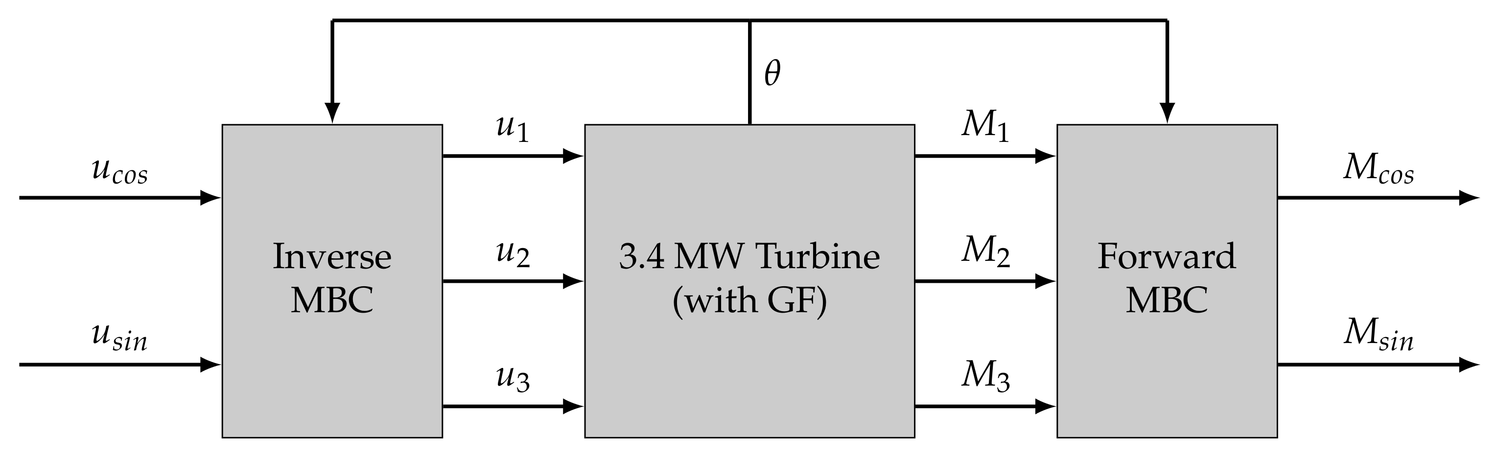
4.2. Multi-Blade Coordinate Transformation

It is known that loads on the turbine blades have the largest component at the 1P harmonic frequency. Thus, a load control system is designed focusing on the harmonic components of the load at 1P and neighboring frequencies. The multi-blade coordinate transformation (MBC) [6] is used to extract the one-per-revolution (1P) harmonic load components from the blade root moment sensors [8]. The MBC assumes that the three turbine blades are identical to each other and located 120 degrees apart. The MBC transformation requires the azimuth angle of the rotor ($\theta$) for the calculation of harmonic load components. Figure 6 shows the wind turbine augmented with the MBC transformations.

The forward MBC transformation is used to map the flapwise root bending moments of the three blades, $M_1$, $M_2$ and $M_3$, from the rotating frame to $M_{cos}$ and $M_{sin}$, the corresponding loads in a fixed frame. The forward MBC transformation can be written as:

$$\left[\begin{array}{c}{M}_{cos}\\ M_{sin}\end{array}\right]=\frac{2}{3}\left[\begin{array}{ccc}cos\theta & cos\left(\theta +\frac{2\pi }{3}\right)& cos\left(\theta +\frac{4\pi }{3}\right)\\ sin\theta & sin\left(\theta +\frac{2\pi }{3}\right)& sin\left(\theta +\frac{4\pi }{3}\right)\end{array}\right]\left[\begin{array}{c}{M}_1\\ M_2\\ M_3\end{array}\right]$$

(1)

where $\theta$ is the azimuth angle (in radians) of the turbine rotor. Under steady wind conditions, the forward MBC transforms the 1P harmonic loads in the rotating frame into constant loads in a fixed frame.

The right inverse of the forward MBC transformation, denoted as “Inverse MBC” block in Figure 6, is utilized to calculate the sectional-lift actuator commands for the three blades, i.e., the rotating frame signals $u_1$, $u_2$ and $u_3$, by transforming the control commands in the fixed frame $u_{cos}$ and $u_{sin}$. The fixed frame control commands are calculated by a feedback controller described in Section 4.6. The inverse MBC transformation can be written as follows:

$$\left[\begin{array}{c}{u}_1\\ u_2\\ u_3\end{array}\right]=\left[\begin{array}{cc}cos\theta & sin\theta \\ cos\left(\theta +\frac{2\pi }{3}\right)& sin\left(\theta +\frac{2\pi }{3}\right)\\ cos\left(\theta +\frac{4\pi }{3}\right)& sin\left(\theta +\frac{4\pi }{3}\right)\end{array}\right]\left[\begin{array}{c}{u}_{cos}\\ u_{sin}\end{array}\right]$$

(2)

The inverse MBC transformation commands the sectional lift actuator of each blade with 1P cosine and sine carrier signals modulated by the control signals $u_{cos}$ and $u_{sin}$. When these latter signals are steady (constant), and the rotor frequency is constant, the rotating frame control signals $u_1,u_2,u_3$ are pure harmonics at 1P. Otherwise, the rotating frame control signals will have spectral content at frequencies other than 1P as well.

The configuration shown in Figure 6 is useful for developing an SLC system that reduces blade-root loads in the rotating frame at 1P and its neighboring frequencies; that is, reduce the blade-root loads in the frequency range 1P $\pm {\omega }_o$, with ${\omega }_o<1$P. In order to reduce the 1P harmonic loads using the MBC transformations, one would need to design a control system to lower the fixed-frame components of the load in the frequency interval $[0,{\omega }_o]$. Recall that the MBC transforms a 1P rotating-frame frequency component to a 0 rad/s fixed-frame frequency component [8,11].

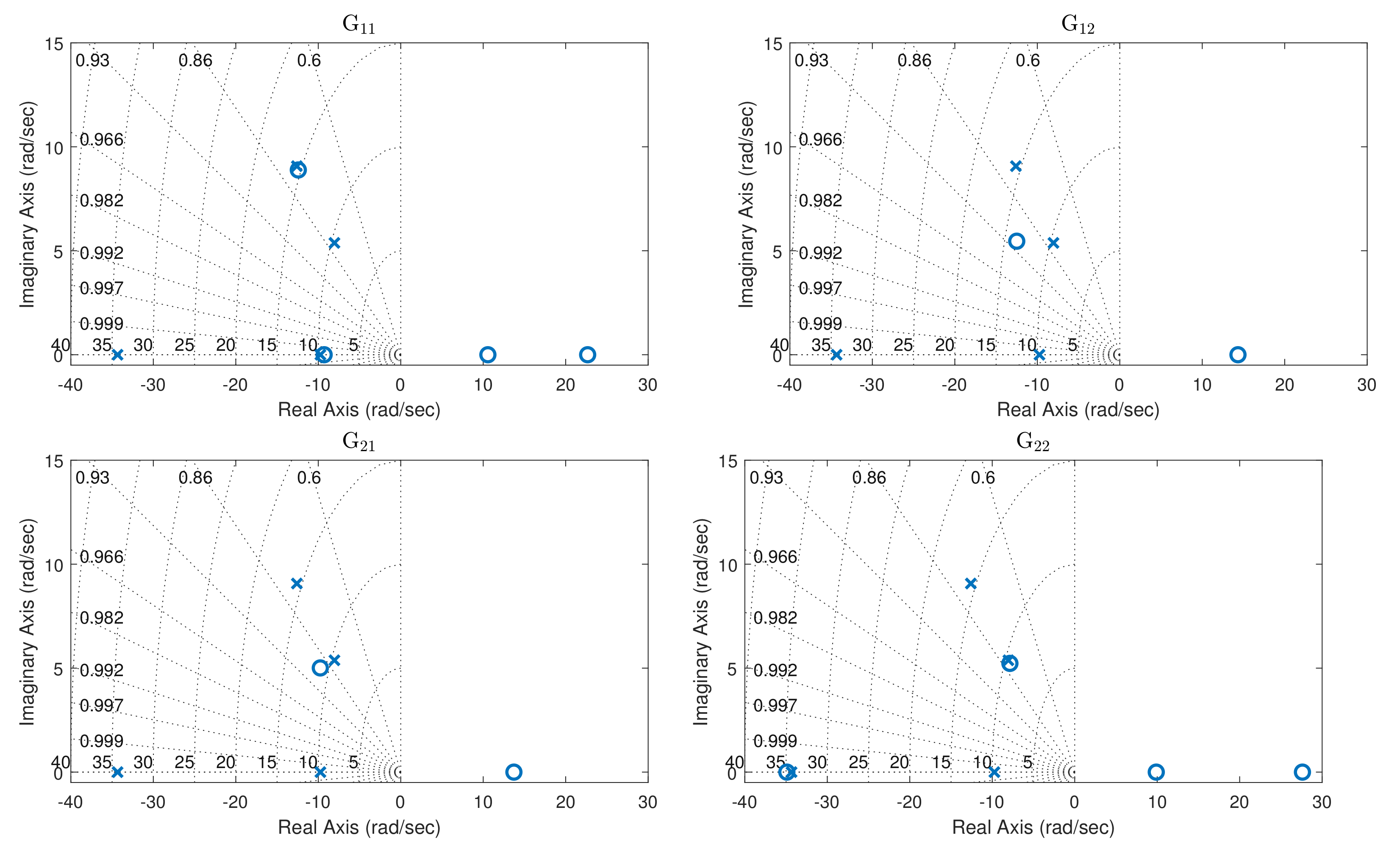
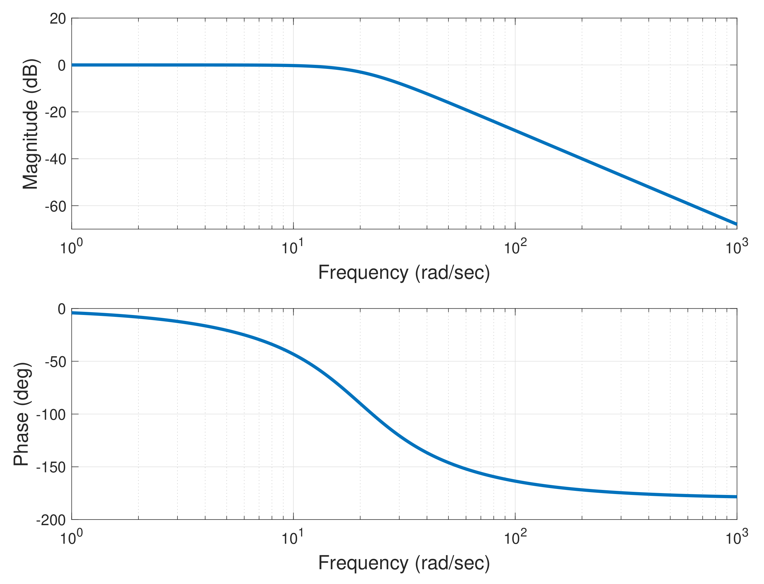
4.3. Design Model via System Identification

A model for the dynamic system with fixed frame input ${\left[u_{cos}{u}_{sin}\right]}^{\prime }$ and fixed frame outputs ${\left[M_{cos}{M}_{sin}\right]}^{\prime }$ is obtained for the design of the SLC. This system is shown in Figure 6. To determine a mathematical model for this system, it is assumed that the wind speed is constant and uniform over the rotor disk. Under this assumption, the open-loop plant model may be assumed (approximately) time invariant, albeit depending on the constant wind speed V impinging on the rotor.

The primary focus of the work described in this article is on designing and utilizing SLC in above-rated wind speeds, when the loads are relatively large. The rated and cut-out wind speeds for the 3.4 MW are 9.8 and 25 m/s, respectively [26]. The design model for developing a robust SLC solution is obtained at $V=18$ m/s, which is close to the midpoint between rated and cut-out wind speeds. A linear state-space model of the open-loop plant at $V=18$ m/s is obtained using the nonlinear simulation data from the modified OpenFAST model of the turbine. The simulations assume uniform wind without any shear or turbulence.

To identify the plant model, it is necessary to excite the plant with appropriate inputs and record the response. Filtered pseudo-random binary signals (PRBS) are chosen as the input to the open-loop plant in Figure 6. A second-order low-pass Butterworth filter with a 3-dB bandwidth of 20 rad/s given by

$$G_{\mathrm{LP}}\left(s\right)=\frac{1}{{(s/20)}^2+\sqrt{2}(s/20)+1}$$

(3)

is used. The frequency response of the low-pass filter is shown in Figure 7. Note that the largest 1P frequency of the rotor is 1.22 rad/s, which corresponds to the rated rotor speed. Thus, a filter with 20 rad/s bandwidth is suitable to identify the relevant open-loop dynamics.

Two independent PRBS signals are filtered by $G_{\mathrm{LP}}$ and the resulting signals applied at the input ${\left[u_{cos}{u}_{sin}\right]}^{\prime }$ of the open-loop plant in Figure 6. The OpenFAST simulations are run for a total of 3000 s, and the first 500 s (98 revolutions) are discarded to remove any initialization effects, resulting in 2500 s (490 revolutions) of usable data. A time step of 0.01 s is chosen for the simulation, which allows estimation of frequency responses up to 50 Hz or 314 rad/s, theoretically.

Figure 8 shows the filtered PRBS inputs signals. The left plots show a small interval (15 s) of the time series signals at the two plant inputs. The corresponding plots on the right show the magnitude of the Fourier transform of the signals. The magnitude of the transfer function of the low pass filter $G_{\mathrm{LP}}$ is shown with a red line. This magnitude is calibrated to match the signal spectrum at low frequency. It can be seen that the frequency content of the signals is focused in the range of 0–10 rad/s and slowly tapers off at higher frequencies as desired, following the magnitude of the low-pass filter.

Table 3. OpenFAST degrees of freedom enabled for system identification.

Degree of Freedom	Description
FlapDOF1	First flapwise blade mode DOF
FlapDOF2	Second flapwise blade mode DOF
EdgeDOF	First edgewise blade mode DOF
DrTrDOF	Drivetrain rotational-flexibility DOF
GenDOF	Generator DOF
TwFADOF1	First fore-aft tower bending-mode DOF
TwFADOF2	Second fore-aft tower bending-mode DOF
TwSSDOF1	First side-to-side tower bending-mode DOF
TwSSDOF2	Second side-to-side tower bending-mode DOF

shows the structural degrees of freedom enabled in the OpenFAST model for system identification. Other degrees of freedom and aerodynamic behavior options like wind shear and tower-blade interaction are also relevant to the control problem but are not enabled in system identification. These latter effects are considered unmodeled disturbances/dynamics and are handled with the robust control method selected for the design of the feedback controller.

The outputs ${\left[M_{cos}{M}_{sin}\right]}^{\prime }$ are logged and the prediction error method (pem function in MATLAB [40]) is used to identify a state-space model from the simulation data. The 2500-s window of usable data is divided into two sets, a 2000-s long “training” dataset and a 500-s long “validation” dataset. The training dataset is used to obtain models of varying orders, which are evaluated for best fit to the validation dataset. The model mismatch is measured with the normalized root mean square error (NRMSE), defined by

$$\mathrm{NRMSE}=\frac{\parallel y_v-y_m{\parallel }_2}{\parallel y_v-mean\left(y_v\right){\parallel }_2}$$

(4)

where $y_v$ is the time series validation data, $y_m$ is the time series predicted by the model, and the ${\ell }_2$ norm of the time series x is defined by

$${\parallel x\parallel }_2=\sqrt{\sum _i{x_i}^2}$$

(5)

The NRMSE for models of different orders, for the case of $V=18$ m/s, is shown in

Table 4. NRMSE for different model orders. Order $n=6$ is optimal.

Model Order	NRMSE
5	0.25
6	0.18
7	0.37
8	0.20

. The model with $n=6$ states is selected as it has the smallest NRMSE with the validation data.

Further insight into the model’s ability to capture essential dynamics at low frequency (up to 3–5 rad/s, approximately) can be obtained from Figure 9. This figure shows the frequency response of the transfer function from the input $u_{cos}$ to the output $M_{cos}$ (see block diagram in Figure 6). The frequency response calculated using the sixth order model shows good fit of the empirical transfer function obtained from the time-series data. The empirical transfer function is obtained using the etfe command provided by the System Identification Toolbox [40] in MATLAB.

Let $G\left(s\right)$ denote the 2×2 transfer matrix from the input ${\left[u_{cos}{u}_{sin}\right]}^{\prime }$ to the output ${\left[M_{cos}{M}_{sin}\right]}^{\prime }$ for the LTI model identified at $v=18$ m/s. Note that the units of $G\left(s\right)$ are kN·m.

We define the four entries of this matrix as follows:

$$G\left(s\right)=\left[\begin{array}{cc}{G}_{11}& G_{12}\\ G_{21}& G_{22}\end{array}\right]$$

(6)

The four entries of the transfer matrix $G\left(s\right)$ are shown in Appendix A. Figure 10 shows the Bode plots of the entries of $G\left(j\omega \right)$. It follows from the figure that $G_{11}\approx G_{22}$ and $G_{21}\approx -G_{12}$, for frequencies $\omega \in [0,10]$ rad/s.

In addition, in this frequency range, we have the imaginary part of $G_{11}\left(j\omega \right)G_{21}^{*}\left(j\omega \right)$ as approximately zero. As a result of this structure, the frequency response of $G\left(j\omega \right)$ is essentially a rotation matrix modulo of a non-unitary magnitude. This structure implies that the two singular values of $G\left(j\omega \right)$ approximately satisfy

$${\sigma }_1\left(G\left(j\omega \right)\right)\approx {\sigma }_2\left(G\left(j\omega \right)\right)\approx \sqrt{|G_{11}{\left(j\omega \right)|}^2+{\left|G_{21}\left(j\omega \right)\right|}^2}$$

(7)

in the interval $\omega \in [0,10]$ rad/s. This, in turn, implies that in this frequency range, inverting the frequency response matrix is a fairly robust operation as its condition number is nearly one. Figure 11 depicts the two singular values of the frequency response matrix $G\left(j\omega \right)$. The Euclidean norm of the first column of the frequency response matrix $G\left(j\omega \right)$, defined in the right-hand side of Equation (7), is also shown with a red dashed line.

The condition number (ratio of maximum to minimum singular value) is shown in Figure 12. These data suggest that inverting the frequency response matrix does not pose a challenge. The inverse of the frequency response matrix is used in the development of the SLC algorithm presented in Section 4.6. More specifically, this transfer matrix is inverted at $\omega =0$ to decouple the control loops at low frequencies.

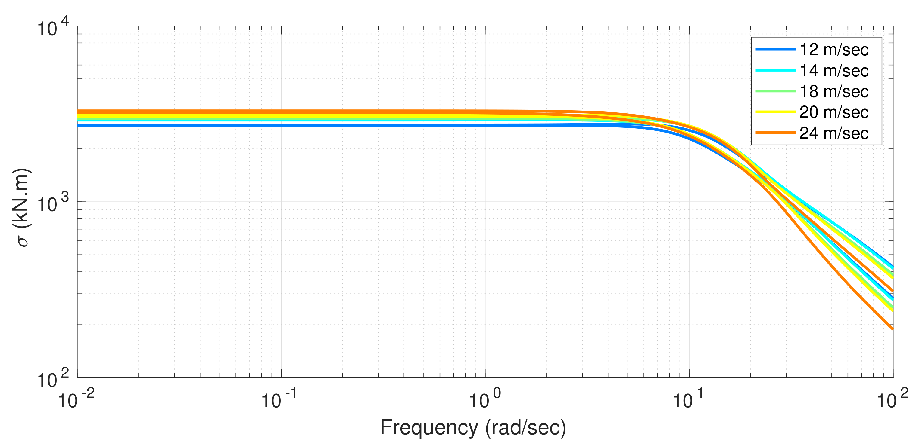
4.4. Variation of Design Model with Wind Speed

Design models for wind speeds other than $V=18$ m/s may be obtained using the system identification procedure described earlier. This section discusses the main properties of the models obtained at various wind speeds and the implications of any model variations on the design of the SLC algorithm for load reduction in above-rated wind conditions (Region-3).

The Bode plots of the four individual transfer matrices are shown in Figure 13 for a range of wind speeds in Region-3.

The singular values of the frequency response matrix $G\left(j\omega \right)$ are shown in Figure 14. With the chosen scales, the frequency responses are clustered together. Note that the frequency responses change slope at the same corner frequencies despite wind speed variations. Thus, for practical purposes, the linear model does not appear sensitive to wind speed variations in Region-3.

A plausible explanation for this behavior is that in above-rated wind conditions, the turbine’s pitch controller is engaged to regulate the rotor angular speed to its rated value. The presence of such feedback loop will reduce the sensitivity to parameter variations of turbine responses, such as the response of blade-root moments to changes in the SLA inputs. As a result, it is natural to expect little variation of the transfer matrix $G\left(s\right)$ with the wind speed V. The practical implication of this observation is that scheduling the control law on wind speed, or other more practical measurement indicative of wind speed, might not have major benefits over a fixed controller. Additional data supporting this observation is provided in Section 5.4.

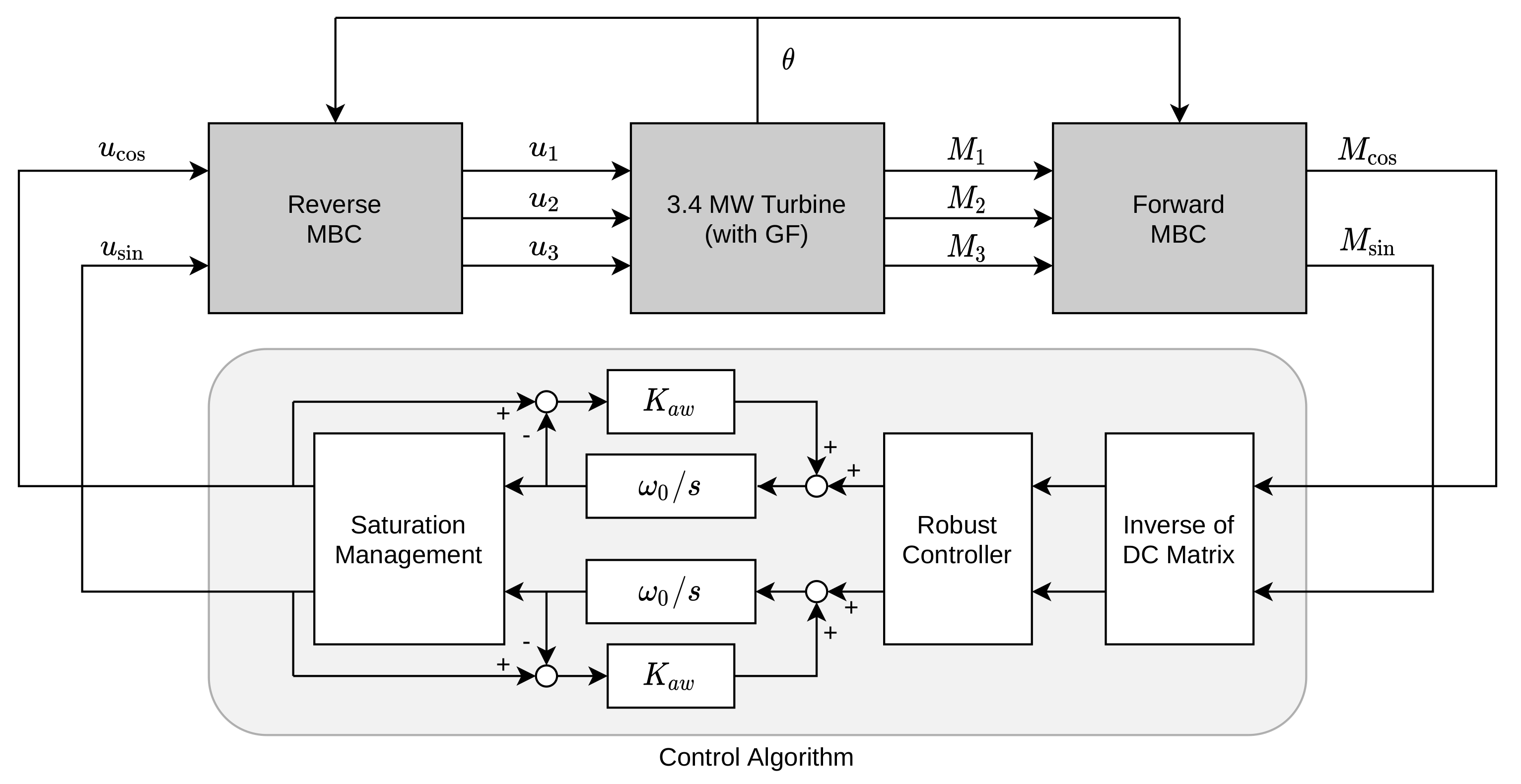
4.5. Sectional Lift Control Architecture

The architecture of the SLC is shown in Figure 15. The control algorithm utilizes the outputs ${\left[M_{cos}{M}_{sin}\right]}^{\prime }$ of the augmented plant to calculate the sectional lift commands in fixed frame ${\left[u_{cos}{u}_{sin}\right]}^{\prime }$. The control algorithm has four basic building blocks. First, the two loops are decoupled at DC, and at low frequencies, by the Inverse of DC Matrix block, which is implemented inverting the DC-gain matrix $G\left(0\right)$ of the identified augmented plant. The Robust Controller block is optional and nominally set to the identity matrix. This block can be designed using $H_{\infty }$ loop-shaping [35] to increase the robustness of the feedback system if desired. The third block is a MIMO diagonal integrator used to achieve disturbance rejection at low frequency; from DC to ${\omega }_0$, approximately. The control signals calculated by the integrators are then modified to take the limited actuator authority of the SLAs into account. This operation is performed by the Saturation Management block in the figure. The block contains a nonlinear scaling, which ensures that the controller commands do not exceed the actuator limits.

Back calculation-based integral anti-windup is also implemented as shown by the blocks with gain $K_{aw}$ in Figure 15. The saturation management block outputs the fixed frame actuator signals ${\left[u_{cos}{u}_{sin}\right]}^{\prime }$, which are then converted to the SLA actuator commands $u_1$, $u_2$ and $u_3$. Details on the design of each block are given in Section 4.6.

4.6. Synthesis of the Control Algorithm

To specify the control algorithm in Figure 15, it is necessary to choose the frequency ${\omega }_0$, the robust controller, the saturation management scheme and the anti-windup gain $K_{aw}$. The selection of ${\omega }_0$ and, if necessary, the robust controller is done using a loop shaping design procedure [35] whereby the augment plant $G\left(s\right)$ is pre- and post-compensated with weights $W_1\left(s\right)$ and $W_2\left(s\right)$, respectively, so that the frequency shaped plant

$$G_s\left(s\right)=W_2\left(s\right)G\left(s\right)W_1\left(s\right)$$

(8)

has desired closed-loop properties as measured by the frequency response of its (two) singular values. In our method, these weights are taken as

$$\begin{array}{cc}\hfill W_1\left(s\right)& =\frac{{\omega }_0}{s}I\hfill \end{array}$$

(9)

$$\begin{array}{cc}\hfill W_2\left(s\right)& =G{\left(0\right)}^{-1}\hfill \end{array}$$

(10)

where I denotes the $2\times 2$ identity matrix. The weight $W_1$ can be seen in Figure 15 following the robust controller block, while the weight $W_2$ is shown following the output of the augmented plant. After a desirable loop shape for $G_s\left(s\right)$ is achieved by selecting ${\omega }_0$, the resulting loop is tested for robust stability.

If robust stability is satisfactory, then the robust controller block is taken to be identity, and the design of the linear elements of the control algorithm is complete. Otherwise, a robust controller with transfer matrix $K_s\left(s\right)$ is obtained by solving the following $H_{\infty }$ optimization problem

$$K_s=argmin{∥\left[\begin{array}{c}I\\ K_s\end{array}\right]{(I+G_s{K}_s)}^{-1}\left[\begin{array}{cc}I& G_s\end{array}\right]∥}_{\infty }$$

(11)

where the minimization is done over all controllers that stabilize $G_s$. The controller $K_s$ is generally of high-order, and its order can and should be reduced to obtain the final robust controller in Figure 15.

Let us elaborate on the selection of the weights $W_1$ and $W_2$. The post-compensator $W_2$ renders the transfer matrix $W_{2}G\left(s\right)$ non-dimensional and equal to the identity matrix at $s=0$. That is, post-compensation is used to decouple and normalize the two control channels at DC. The calculation of $W_2=G{\left(0\right)}^{-1}$, and its use as a post-compensator, is numerically stable and remarkably robust given that the condition number of $G\left(j\omega \right)$ is close to one at low frequencies (cf. Figure 12). The singular values of $W_{2}G\left(j\omega \right)$ are shown in Figure 16. Note that they are exactly one at $\omega =0$, and remain close to one for low frequencies. Thus, in order to reduce the fixed-frame moments $M_{cos}$ and $M_{sin}$ for frequencies ranging from DC to a low-frequency ${\omega }_0$, it suffices to select an integral pre-compensator $W_1$, as shown in Equation (9). For all practical purposes, ${\omega }_0$ is the cross-over frequency of magnitude for $G_s$. Hence, if robust stability can be achieved with the robust controller $K_s=I$, ${\omega }_0$ will be the closed-loop bandwidth. That is, ${\omega }_0$ defines the frequency range where load reduction of fixed-frame moments will occur. Given this argument, we recommend taking $0.2P\le {\omega }_0<1P$, where $1P$ is the rated turbine rotor frequency.

To complete the design method, we need to define the criteria for robust stabilization of the shaped plant $G_s$. We use the normalized coprime factor stability margin [34] defined by

$${ϵ}_s=\frac{1}{\sqrt{2}{∥{(I+G_s)}^{-1}\left[\begin{array}{cc}I& G_s\end{array}\right]∥}_{\infty }}$$

(12)

Based on experience, we take the minimum acceptable stability margin to be 0.4. That is, if ${ϵ}_s>0.4$, the robust controller block in Figure 15 is set to be the identity matrix. Otherwise, we design the robust controller from Equation (11) and possibly include a controller order reduction step. Note that our threshold for the stability margin exceeds the recommended value ${ϵ}_s>0.33$ [41] to increase robustness to modeling uncertainty.

The significance of the normalized coprime factor stability margin in Equation (12) may be understood with the aid of the block diagram in Figure 17. In this figure, ${\Delta }_1$ and ${\Delta }_2$ are dynamic perturbations that represent inverse multiplicative uncertainty at plant output and direct multiplicative uncertainty at plant input. It is well-known that the block ${\Delta }_1$ can capture modeling uncertainty and/or parametric variations, e.g., pole migrations due to changes in operating conditions such as the wind speed. On the other hand, the block ${\Delta }_2$ may capture unmodeled dynamics, such as unsteady aerodynamic effects due to sectional lift actuation using plasma-based devices. See [41] for further details on uncertainty modeling. It turns out that the feedback loop in Figure 17 is (internally stable) if and only if

$${∥\left[\begin{array}{c}{\Delta }_1\\ {\Delta }_2\end{array}\right]∥}_{\infty }<\sqrt{2}{ϵ}_s$$

(13)

Loosely speaking, if ${ϵ}_s>0.4$, then the feedback system in Figure 17 can tolerate modeling uncertainty as large as 57% at all frequencies without losing stability.

Further insight on the interpretation of ${ϵ}_s$ follows from the bounds it provides for classical single-input single-output (SISO) stability margins. While this is not our case, these SISO bounds are informative. More specifically, a given normalized coprime stability margin ${ϵ}_s$ provides the bounds on the gain and phase margin shown in Equation (14) [34].

$$\begin{array}{c}\hfill \begin{array}{cc}\hfill GainMargin& \ge \frac{1+{ϵ}_s}{1-{ϵ}_s}\hfill \\ \hfill PhaseMargin& \ge 2arcsin\left({ϵ}_s\right)\hfill \end{array}\end{array}$$

(14)

For example, a coprime stability margin ${ϵ}_s=0.4$ guarantees a gain margin of 2.33 and a phase margin of 47 degrees, which are acceptable values for SISO loops.

Now, we provide the details of our SLC design for the 3.4 MW turbine. The design model is given by the augmented plan $G\left(s\right)$ as identified at 18 m/s wind speed. The choice of the bandwidth ${\omega }_0$ is based on the reduction in the damage equivalent load of the flapwise root bending moments on the turbine blades. In order to choose the bandwidth, controllers were designed and tested with turbulent wind. The ${\omega }_0$ value that provides the most load reduction is selected. Based on this analysis, the bandwidth is chosen to be ${\omega }_0=0.3\times 1P=0.37$ rad/s.

Once a numerical value for ${\omega }_0$ is known, the shaped plant $G_s$ in Equation (8) is known and we may compute its stability margin using Equation (12). For our plant, we obtained ${ϵ}_s=0.62$. This implies that the control system is robust and $H_{\infty }$ loop-shaping based modifications are not needed. Thus, the final controller is a MIMO integral controller of the form

$$K\left(s\right)=W_1\left(s\right)W_2=\left[\begin{array}{cc}\frac{{\omega }_0}{s}& 0\\ 0& \frac{{\omega }_0}{s}\end{array}\right]G{\left(0\right)}^{-1}$$

(15)

Figure 18 shows the singular value plots of the open-loop transfer matrix $L\left(s\right)=G\left(s\right)K\left(s\right)$ for the control loop broken at plant output, the closed-loop sensitivity $S\left(s\right)={(I+L\left(s\right))}^{-1}$ and complementary sensitivity $T\left(s\right)=L\left(s\right)S\left(s\right)$. Load reduction is expected to occur for frequencies up to 0.4–0.5 rad/s because the sensitivity is less than one in this range of frequencies. The peak value of the sensitivity is ${\parallel S\parallel }_{\infty }=1.11$, and the peak value of the complementary sensitivity is ${\parallel T\parallel }_{\infty }=1$, well below recommended values [34].

The linear component of the control algorithm in Figure 15 was designed using the plant model identified at a wind speed of 18 m/s. The same design process can be used to design linear controllers for plants at other wind speeds. The controllers thus obtained can be utilized to obtain an SLC scheduled on wind speed. Section 5.4 demonstrates the results of this approach. No significant benefits are observed with the scheduled SLC in terms of load reduction or stability margin or performance to justify the added complexity of scheduling control parameters on wind speed. Therefore, the results presented in the rest of the paper are based on the controller designed at 18 m/s, as shown in Equation (15).

Saturation Management

In this paper, we assume that the actuator limits are $\pm 0.2$. These limits on the sectional lift coefficient (i.e., actuator) are within reach of future plasma technology [7,25]. Following Reference [42], nonlinear scaling is applied to the control signals calculated by the controller, as shown on Figure 15. The purpose of the scaling is to modify the output of the controllers so that they remain within the actuator limits while providing suitable load reduction. Denote the inputs to the nonlinear scaling block as $v_{cos}\left(t\right)$ and $v_{sin}\left(t\right)$, while the outputs are $u_{cos}\left(t\right)$ and $u_{sin}\left(t\right)$. The scaling can be described as follows

$$\begin{array}{c}\hfill \begin{array}{cc}\hfill u_{cos}\left(t\right)& =\left\{\begin{array}{cc}\frac{v_{cos}\left(t\right)}{\sqrt{v_{cos}{\left(t\right)}^2+v_{sin}{\left(t\right)}^2}}\times 0.2\hfill & \mathrm{if}\sqrt{v_{cos}{\left(t\right)}^2+v_{sin}{\left(t\right)}^2}>0.2\hfill \\ v_{cos}\left(t\right),\hfill & \mathrm{otherwise}\hfill \end{array}\right.\hfill \\ \hfill u_{sin}\left(t\right)& =\left\{\begin{array}{cc}\frac{v_{sin}\left(t\right)}{\sqrt{v_{cos}{\left(t\right)}^2+v_{sin}{\left(t\right)}^2}}\times 0.2\hfill & \mathrm{if}\sqrt{v_{cos}{\left(t\right)}^2+v_{sin}{\left(t\right)}^2}>0.2\hfill \\ v_{sin}\left(t\right),\hfill & \mathrm{otherwise}\hfill \end{array}\right.\hfill \end{array}\end{array}$$

(16)

It should be noted that the scaled inputs always have the following property.

$$\sqrt{u_{cos}^2+u_{sin}^2}\le 0.2$$

(17)

The constraint shown in Equation (17) on the fixed frame control signal implies that the corresponding control signals in the rotating frame are always within the range of $\pm 0.2$, which satisfies the actuator constraint. This scaling method is non-conservative (i.e., it uses the full actuator authority) because the magnitude of each actuator command satisfies $max|u_i|=\sqrt{u_{cos}^2+u_{sin}^2}$. Furthermore, scaling the control signals in the fixed frame, prior to applying the MBC transformation to obtain the actual actuator commands, ensures that at every time instant, the sum of all the actuator commands is zero, which is necessary to avoid undesirable changes on the collective lift on the blades.

When the output of the scaling function saturates, the system in Figure 15 becomes open-loop. The two integrators in the controller would windup unless this saturation is detected and acted upon. A simple back-calculation anti-windup scheme [43] is implemented to ensure the integrator outputs $v_{cos}\left(t\right)$ and $v_{sin}\left(t\right)$ track the scaled signals $u_{cos}\left(t\right)$ and $u_{sin}\left(t\right)$ to avoid integrator windup. The anti-windup gain $K_{aw}$ is non-dimensional and determines the bandwidth of the anti-windup loops. A unit value for $K_{aw}$ implies a bandwidth comparable to the SLC. Typically, this gain would need to be much larger than one. After trial and error, we take $K_{aw}=100$. The parameters of the final SLC controller are shown in

Table 5. Parameters of the SLC controller.

Parameter	Value
Actuator Limits	−0.2 to +0.2
$K_{aw}$	100
${\omega }_0$ (rad/s)	0.37
DC-gain $G\left(0\right)$ (kN·m)	$\left[\begin{array}{cc}2.7033\times {10}^3& -1.2389\times {10}^3\\ 1.2486\times {10}^3& 2.7590\times {10}^3\end{array}\right]$
Robust Controller	I (Identity Matrix)

.

5. Loads and Performance Evaluation

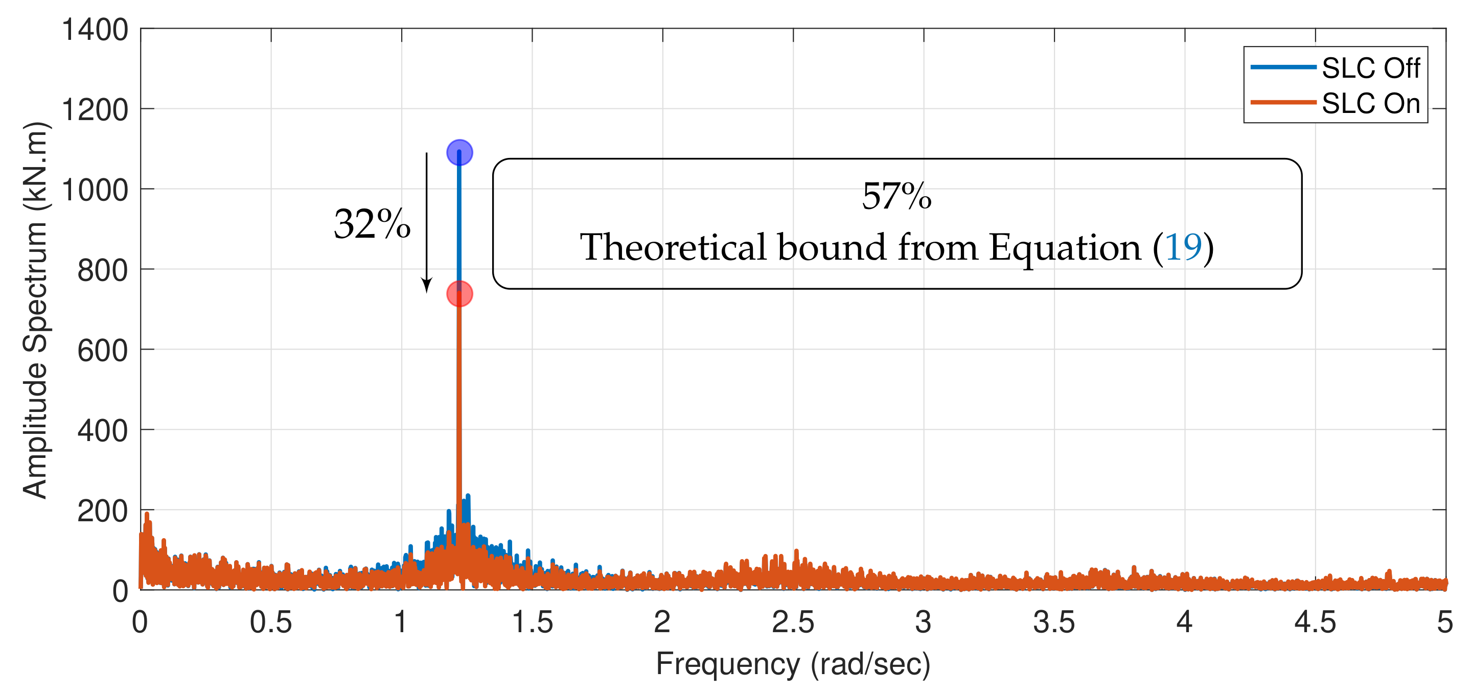
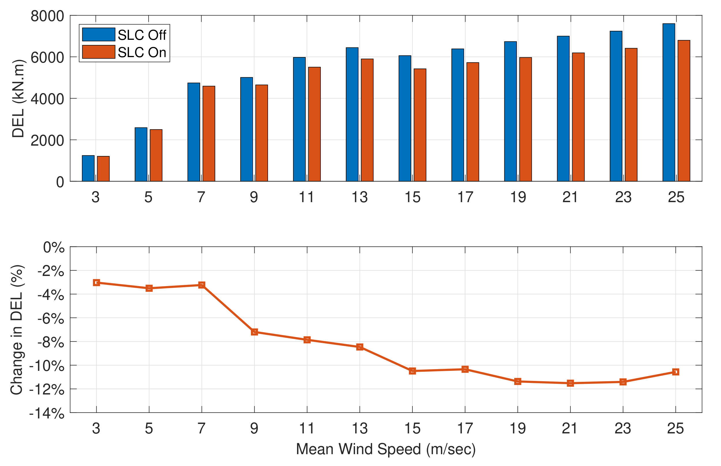
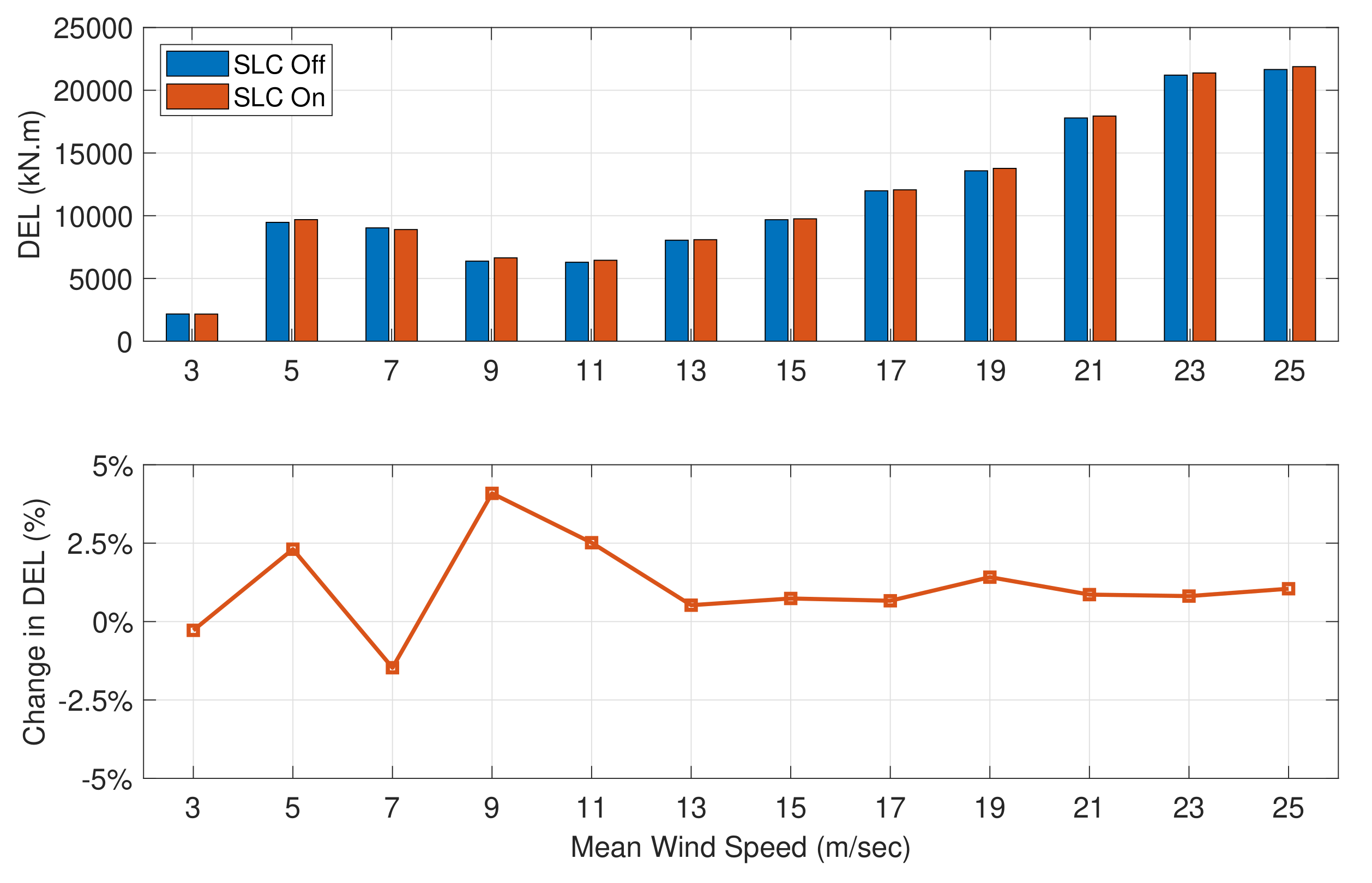
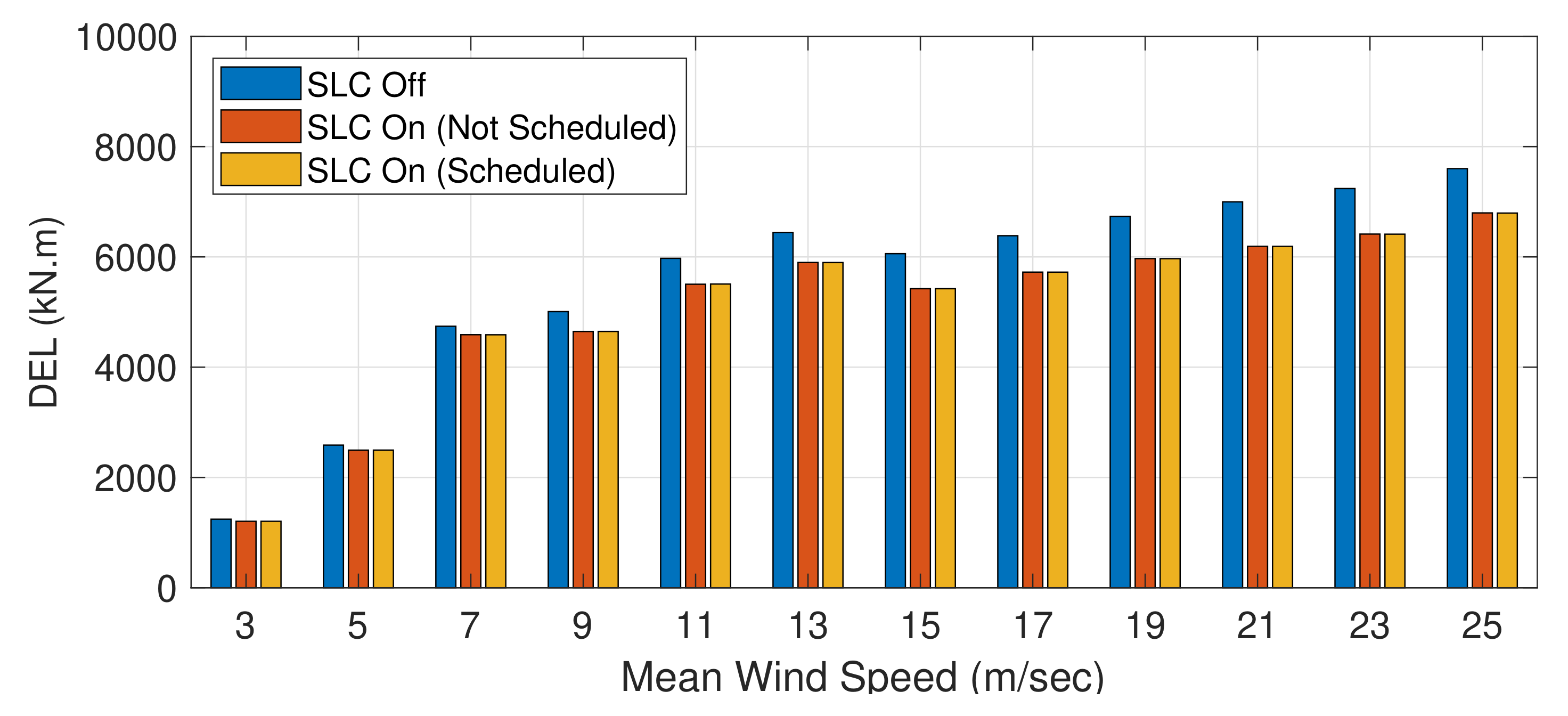
The performance of the control system shown in Figure 15, with the parameters given in Table 5, is analyzed by comparing the evaluation criteria in Table 2 with and without SLC. Damage equivalent load (DEL) [38] provides a measure of the fatigue due to various dynamic loads on a wind turbine. The DELs of the moments are analyzed based on the IEC standard design load case 1.2 [28]. Simulations are run for the full operational range of the turbine. The software TURBSIM [44] is used to generate eight different turbulent wind files for each mean wind speed. The DELs for various loads are calculated using MLife [39]. Turbine performance is also evaluated to determine what impact, if any, the SLC has on the power produced, the rotor angular speed and the collective pitch activity.

5.1. Primary Load

The primary objective of the SLC is to reduce the flapwise root bending moments on the turbine blades. The SLC impact on these loads is evaluated with steady and turbulent wind. Figure 19 shows the effect of the load control system on the blade flapwise root bending moment for 18 m/s steady wind with vertical shear exponent $\alpha =0.2$. The top plot shows the time series of the actuator command where the SLC is switched on at 400 s. The middle plot shows the corresponding time series of the bending moment. A 37% reduction in the peak-to-peak value of the moment signal is observed. The frequency domain plot at the bottom of Figure 19 shows a 43% reduction of the 1P harmonic component. There are very small changes in the 2P, 3P and other higher components.

The change in the bending moment signals is also observed for the case of turbulent wind and vertical wind shear. This is shown in Figure 20. A 32% reduction is observed in the 1P harmonic component along with reductions in a frequency range within 1P ±${\omega }_0=1.22\pm 0.37$ rad/s. This is expected because the bandwidth of the SLC is chosen as ${\omega }_0=0.37$ rad/s.

Figure 19 and Figure 20 also show the theoretical lower bounds for load reduction. These bounds are obtained from the following result, which is proven in Appendix B.

Lemma 1.

Let $G\left(0\right)$ denote the DC-gain of the MBC augmented plant defined in Figure 6 at wind speed V. Assume that the singular values of $G\left(0\right)$ are ${\sigma }_1\ge {\sigma }_2$. Assume also that the feedback system in Figure 15 is in periodic steady-state with a 1P fundamental frequency in blade coordinates ($M_1,M_2,M_3$). Let $M_{1P}^{ol}$ and $M_{1P}^{cl}$ denote the open and closed-loop 1P amplitude of the blade root flapwise bending moment at V, where the closed-loop response $M_{1P}^{cl}$ is obtained with the controller in Figure 15. Then, the 1P closed-loop response $M_{1P}^{cl}$ is bounded below as follows:

$$M_{1P}^{ol}-{\sigma }_1{u}_{\max }\le M_{1P}^{cl}$$

(18)

where $u_{\max }=0.2$ is the authority of the SLA.

From this result, it follows that the %-load reduction $\delta =100\times \left(1-M_{1P}^{cl}/M_{1P}^{ol}\right)$ cannot exceed the upper bound

$$\delta \le 100\left(\frac{{\sigma }_1}{M_{1P}^{ol}}\right)u_{\max }$$

(19)

Note that when $M_{1P}^{ol}>{\sigma }_1{u}_{\max }$, the amplitude of the open-loop disturbance exceeds the actuator authority required to fully reject the open-loop disturbance. To explain this point, consider an additive constant disturbance load vector d at the output of the generalized plant G in Figure 15, with ${\parallel d\parallel }_2=M_{1P}^{ol}$. Thus, d represents the 1P cosine and sine component of the open load. Then, the closed-loop loads in the fixed frame are given by

$$\left[\begin{array}{c}{M}_{cos}\\ M_{sin}\end{array}\right]=G\left(0\right)\left[\begin{array}{c}{u}_{cos}\\ u_{sin}\end{array}\right]+d$$

(20)

Thus, if $M_{1P}^{ol}>{\sigma }_1{u}_{\max }$, then ${\parallel d\parallel }_2>{\sigma }_1{u}_{\max }$, which in turn implies that ${\parallel G\left(0\right)}^{-1}{d\parallel }_2>u_{\max }$. This last inequality shows that $M_{cos}=M_{sin}=0$ is not achievable regardless of the controller used. On the other hand, when ${\parallel G\left(0\right)}^{-1}{d\parallel }_2\le u_{\max }$, the controller in Figure 15 does not saturate and due to the integral control component, the closed-loop response vanishes in steady state, achieving full load reduction, i.e., $M_{1P}^{cl}=\sqrt{M_{cos}^2+M_{sin}^2}=0$.

The DEL for the blade flapwise root bending moment is also calculated for turbulent wind conditions with vertical shear, according to the IEC standard. Figure 21 shows this DEL with and without SLC.

It can be seen that SLC is able to reduce the DEL for the blade flapwise root bending moment, i.e., the primary load targeted by the control system. To quantify the impact of the SLC on the DEL, the following % change used:

$${\mathrm{DEL}}_{\mathrm{bad} \mathrm{hbox}}=\frac{\left({\mathrm{DEL}}_{\mathrm{SLC}}\mathrm{On}-{\mathrm{DEL}}_{\mathrm{SLC}}\mathrm{Off}\right)}{{\mathrm{DEL}}_{\mathrm{SLC}}\mathrm{Off}}\times 100$$

(21)

The % change in DEL for a range of mean wind speeds is shown in the bottom plot of Figure 21. It can be seen that the load control system achieves a reduction up to around 12% depending on the wind speed. Higher reductions in DEL are observed for above-rated wind speeds as compared to below-rated wind speeds.

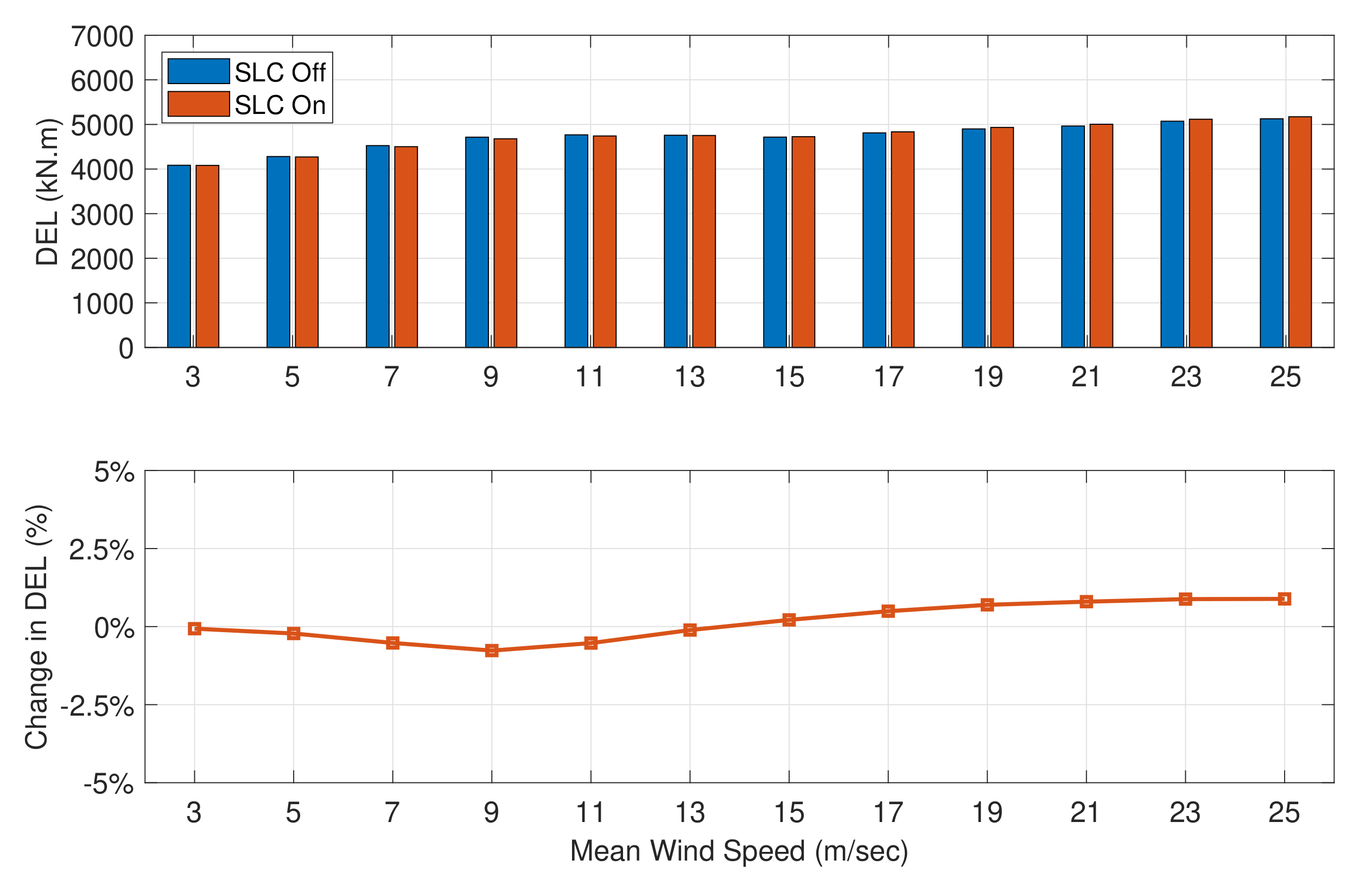
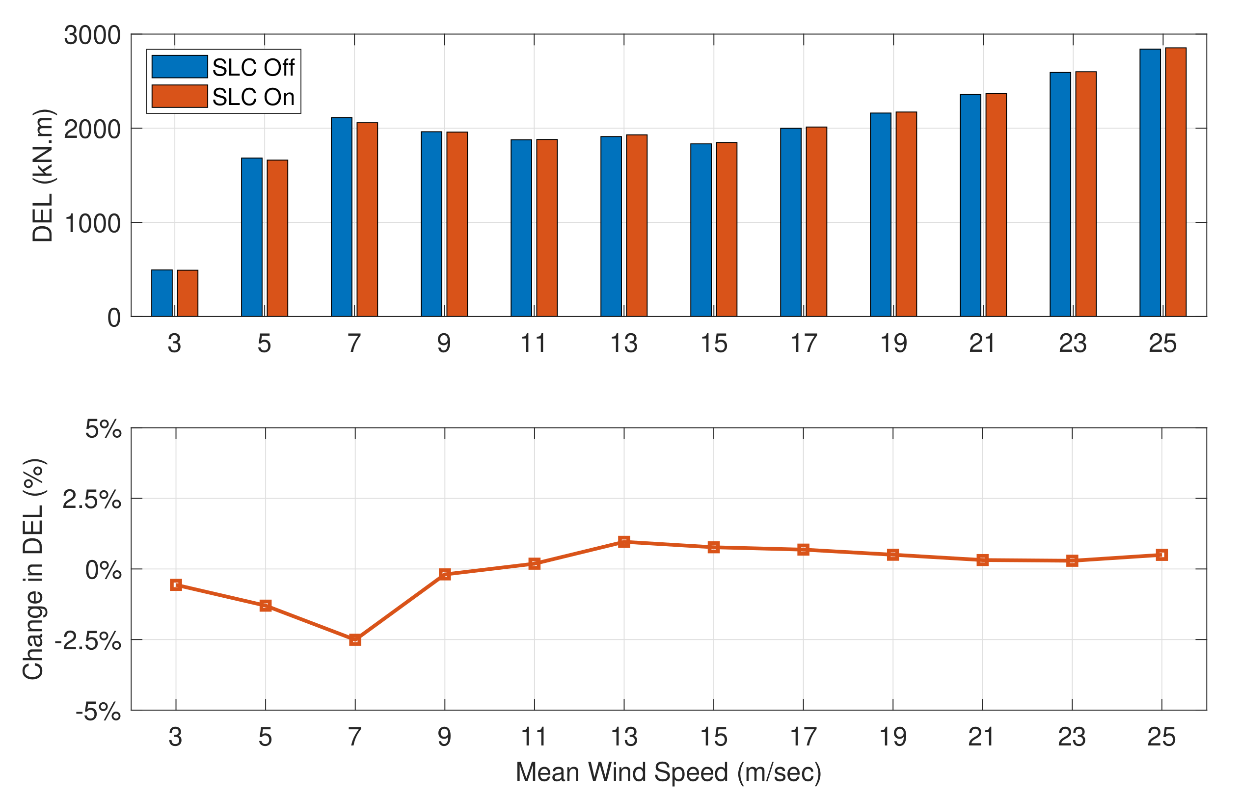
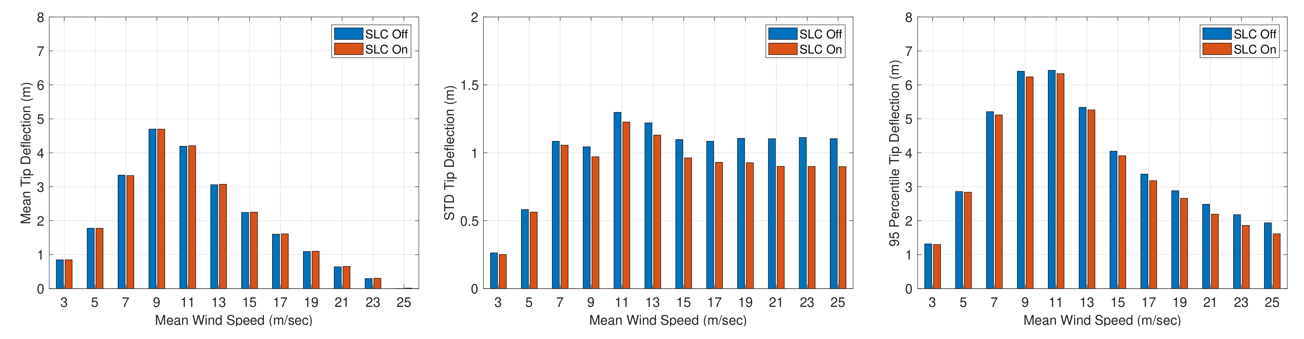
5.2. Secondary Loads

The effect of SLC on the secondary loads on the wind turbine is evaluated as well. Ideally, the secondary loads should either decrease or not be affected. DEL and % change in DEL are used to measure the effect of SLC on these secondary loads. Figure 22 shows the DEL for the blade root edgewise bending moment with and without SLC. The SLC has a very small effect on the edgewise moments. This is also evident by the fact that % change in DEL is almost zero for all wind speeds.

A similar conclusion can be drawn about the tower base moments. Figure 23 shows the DEL and % change in DEL for the tower base fore-aft moment, while Figure 24 shows the same criteria for the tower base side-side moment. Note that the effect of the SLC on these loads is not significant.

Next, we compare the blade tip deflection with and without SLC. Figure 25 shows the variation of the mean, standard deviation and the 95th percentile of blade tip deflection with wind speed. These metrics are calculated using the data from the eight random simulations; thus, the 95th percentile is a more reliable indicator of large deflections than the actual maximum deflection. As expected, tip defection grows up to the rated wind speed (9.8 m/s) and then decays because the turbine “pitches-to-feather” to regulate rotor speed. As expected, the SLC does not affect the mean value of the tip displacement. However, there is reduction in the spread (standard deviation) and the 95th percentile of the displacement values under the SLC. This implies that reducing dynamic fluctuating loads leads to a reduction in dispersion and peak values of tip deflection.

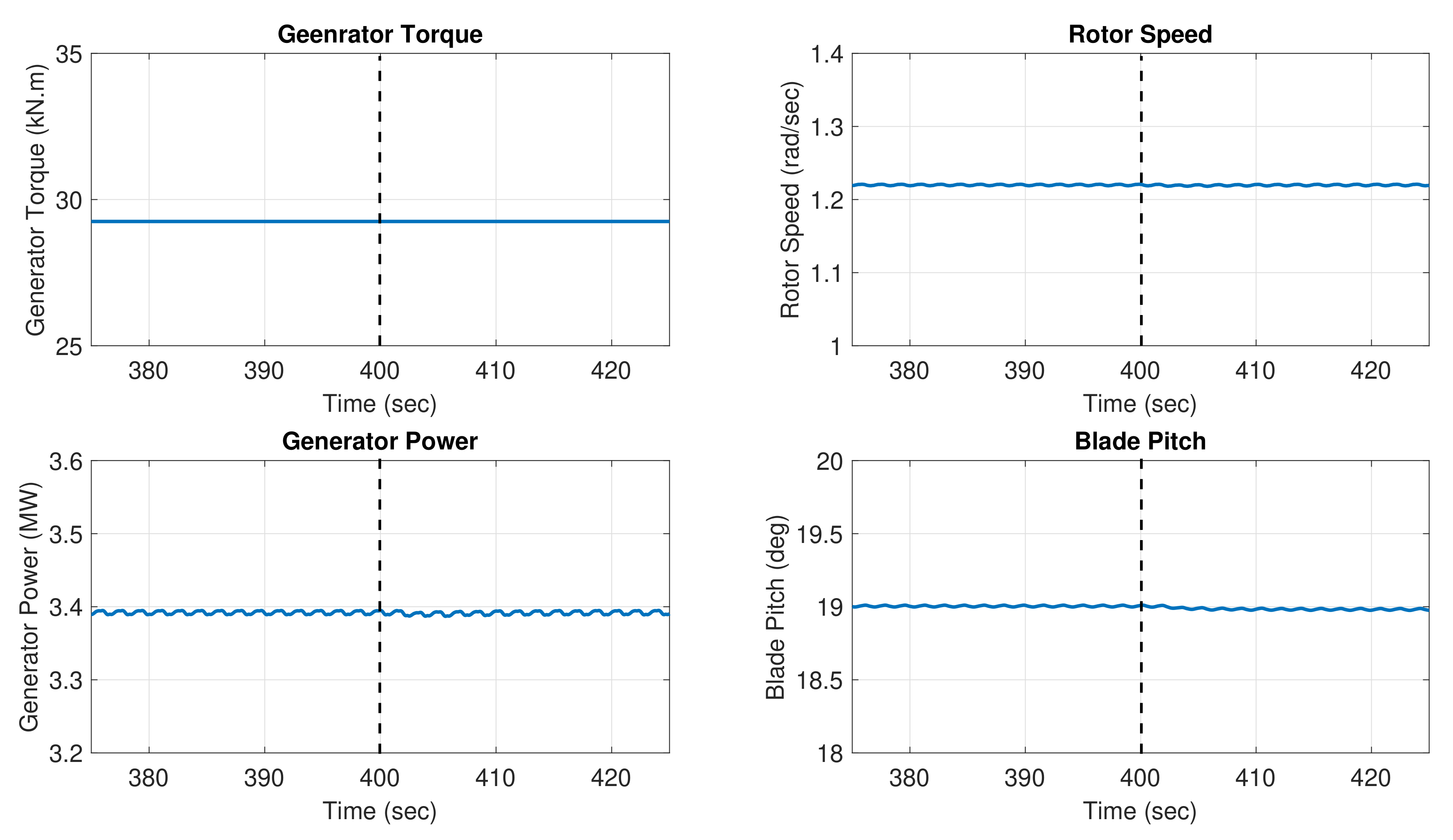
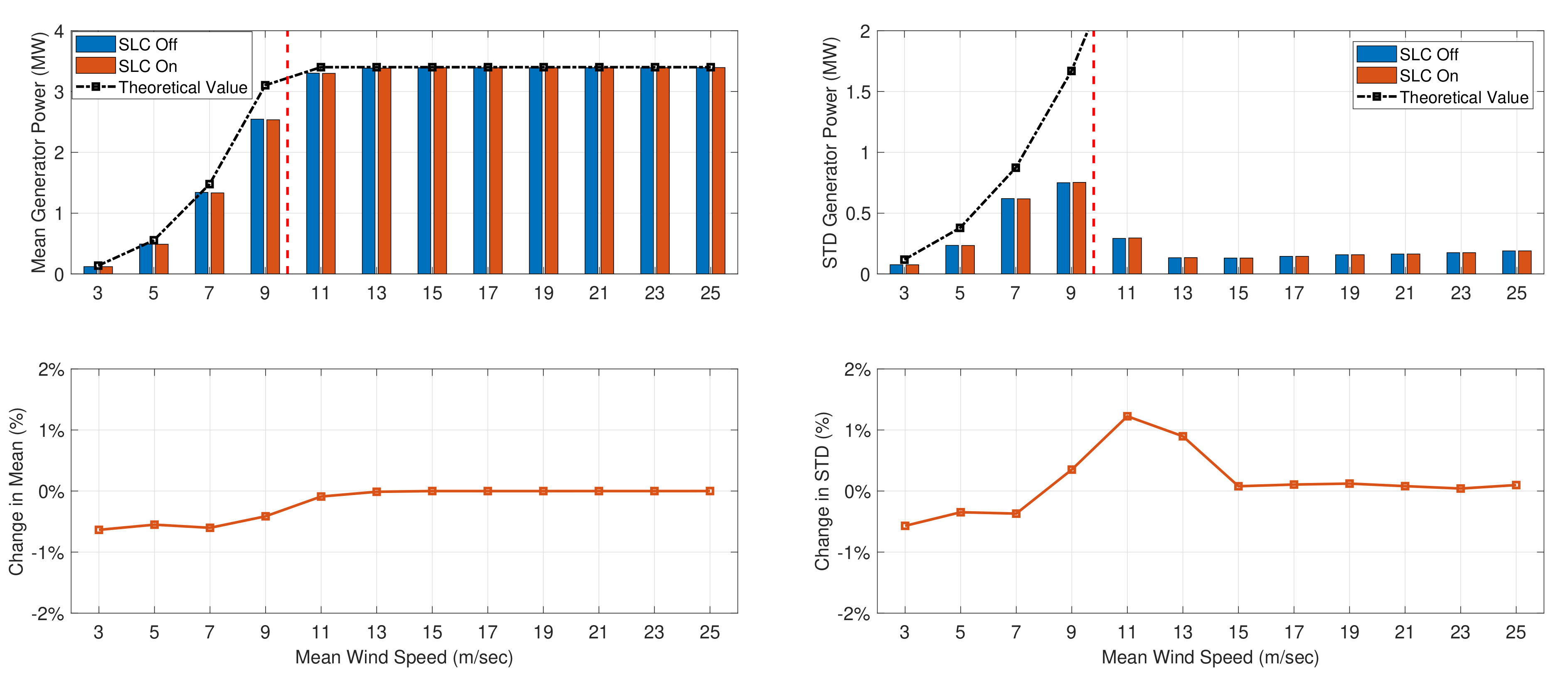
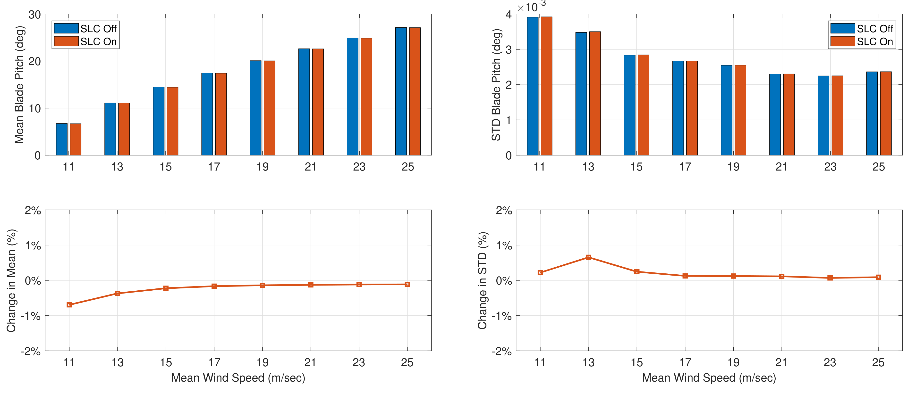
5.3. Turbine Activity

First, we demonstrate that the SLC does not have any impact on turbine performance by evaluating the relevant time series at a particular wind condition. Figure 26 shows the time domain signals from the turbine for a steady wind of 18 m/s with vertical wind shear $\alpha =0.2$. The controller is switched on at 400 s. The figure shows that the SLC does not affect the turbine performance. The rotor speed, blade pitch, generator torque and power show similar behavior before and after SLC is activated. This is expected because at any instant, the sum of the lift generated by the actuators on the three blades is zero. Moreover, the sum of the corresponding moments due to these lifts is also zero as the actuators are located at the same spanwise position on the three blades. Thus, the fixed frame quantities, similarly to turbine performance, are not affected by the SLC.

The effect of the SLC on turbine performance is evaluated for turbulent wind as well by analyzing the mean and standard deviation (STD) of the sample distributions resulting from the eight random simulations performed to analyze loads. Figure 27 shows the comparison of the mean and STD of the generator power with and without SLC. This figure also shows the theoretical mean and STD calculated using the turbine’s maximum power coefficient ($C_{p,max}=0.47$) and the sample statistics of $V^3$ (mean and STD). The rated wind speed is indicated with a vertical dashed red line at 9.8 m/s. The change in the mean and the STD are plotted at the bottom of the figure. Minor changes (<2%) are observed in the mean and STD of the power with SLC, and it can be concluded that SLC does not affect the turbine power in any significant manner.

Similarly, the mean and STD of the rotor speed are compared, as shown in Figure 28. The SLC results in less than 1% changes in these metrics for the rotor speed. The turbine controller keeps the blade pitch constant for below-rated wind speeds. Thus, to evaluate the impact of the SLC on the pitch system, the mean and the STD of the blade pitch are compared for the above-rated wind speeds, as shown in Figure 29. Again, the SLC shows <1% change in the blade pitch parameters.

5.4. Scheduling the SLC with Wind Speed

This section shows results for an SLC controller scheduled with wind speed. The scheduled controller is obtained by applying the system identification procedure in Section 4.3 to determine linear models at 12 wind speeds ranging from 3 to 25 m/s. Then, for each plant model, a MIMO integral controller, as shown in Equation (15), is defined using ${\omega }_0=0.37$ rad/s and the DC-gain $G\left(0\right)$, which is a function of the wind speed V.

Figure 30 shows the DELs for the flapwise blade root bending moments where we compare the controller designed using the model obtained at 18 m/s (red) with the controller scheduled on wind speed (yellow). Note that the scheduled controller results in nearly identical DELs as compared to the single controller designed at 18 m/s. Thus, the added complexity required to schedule the controller on wind speed is not justified.

6. Conclusions

This paper described a methodology for the design of a dynamic feedback control system to reduce blade fatigue loads. This approach, which we have coined sectional lift control (SLC), uses the local lift coefficient to model on-blade active flow control devices such as controllable Gurney flaps based on DBD plasma actuators. The SLC architecture is based on the well-known multi-blade coordinate transformation (MBC), which allows the reduction of blade loads within a neighborhood of the fundamental rotor angular frequency (1P).

Salient features of our methodology include:

• The SLC is model-based and can be designed from simple approximate models (physics-based or data) due to the explicit incorporation of a robust stability margin to both parametric uncertainty and unmodeled dynamics.
• The SLC does not interact with the main turbine controller and reduces the controlled loads in below- and above-rated wind conditions, without adverse impacts on turbine power or blade pitch activity.
• The methodology is directly applicable to an actual wind turbine equipped with DBD plasma actuators (or other flow control devices) by using system identification tools to obtain a model from the actuator signals (voltage for DBD plasma actuators) to the controlled moments.

The design methodology is demonstrated using an OpenFAST model of a 3.4 MW wind turbine equipped with a controllable Gurney flap, controlled via plasma actuation, to reduce the blade-root flapwise bending moments. The study shows that fatigue loads, as measured by DELs of the flapwise bending moments, can be reduced from 4% to 8% in below-rated wind speeds and from 8% to 12% in above-rated wind conditions. Secondary loads, such as blade-root flapwise bending and tower fore-aft bending moments, are not affected by the SLC. The tip deflection in response to stochastic wind inputs is evaluated as well. The statistical analysis of the data shows that the SLC reduces the 95% percentile of the tip deflection and its dispersion about the mean.

It is also shown that a single SLC designed at a specific above-rated wind speed (18 m/s in this case) suffices to control loads from cut-in to cut-out wind speed. This result suggests that there is no need to gain-schedule the SLC on wind speed or another correlated measurement. For above-rated wind speeds, this hypothesis has a control-theoretic explanation. In this case, the main turbine controller is designed to regulate the power and rotor speed to rated values. This feedback loop reduces the sensitivity of wind turbine input/output transfer functions to parameter (e.g., wind speed) variations. Thus, the transfer function from changes in local lift to blade-root moments is relatively independent of wind speed in the bandwidth of interest.

In the companion work [27], the 3.4 MW turbine re-designed with the controllable GF, controlled with the SLC presented in the current paper, was compared to the baseline reference IEA 3.4 MW turbine from Reference [26]. This comparison shows LCOE reduction of 3.5–5.9%, a range based on analysis of different OPEX assumptions. These LCOE savings are derived from capital costs reductions due to wind turbine load reductions in this re-design scenario as the re-designed rotor with Gurney flap (GF) includes minimal AEP increase. As noted in [27], and in part in Section 5, this GF-based active load control system results not only in blade load reductions but also load reductions in other major components (including the pitch system, drive-train, and yaw system)—significant reduction in both capital costs and operational costs result from these load reductions.

References

1. McKenna, R.; vd Leye, P.O.; Fichtner, W. Key challenges and prospects for large wind turbines. Renew. Sustain. Energy Rev. 2016, 53, 1212–1221. [Google Scholar] [CrossRef]
2. Bossanyi, E.A. Individual blade pitch control for load reduction. Wind Energy Int. J. Prog. Appl. Wind Power Convers. Technol. 2003, 6, 119–128. [Google Scholar] [CrossRef]
3. Bossanyi, E.A. Further load reductions with individual pitch control. Wind Energy Int. J. Prog. Appl. Wind Power Convers. Technol. 2005, 8, 481–485. [Google Scholar] [CrossRef]
4. Caselitz, P.; Kleinkauf, W.; Krüger, T.; Petschenka, J.; Reichardt, M.; Störzel, K. Reduction of fatigue loads on wind energy converters by advanced control methods. In Proceedings of the European Wind Energy Conference, Dublin Castle, Ireland, 6–9 October 1997; pp. 555–558. [Google Scholar]
5. Zhang, Y.; Chen, Z.; Cheng, M. Proportional resonant individual pitch control for mitigation of wind turbines loads. IET Renew. Power Gener. 2013, 7, 191–200. [Google Scholar] [CrossRef]
6. Bir, G. Multi-blade coordinate transformation and its application to wind turbine analysis. In Proceedings of the 46th AIAA Aerospace Sciences Meeting and Exhibit, Reno, NV, USA, 7–10 January 2008; p. 1300. [Google Scholar]
7. Liu, C.; Li, Y.; Cooney, J.A.; Fine, N.E.; Rotea, M.A. NREL FAST modeling for blade load control with plasma actuators. In Proceedings of the 2018 IEEE Conference on Control Technology and Applications (CCTA), Copenhagen, Denmark, 21–24 August 2018; pp. 1644–1649. [Google Scholar]
8. Lu, Q.; Bowyer, R.; Jones, B.L. Analysis and design of Coleman transform-based individual pitch controllers for wind-turbine load reduction. Wind Energy 2015, 18, 1451–1468. [Google Scholar] [CrossRef] [Green Version]
9. Leithead, W.; Neilson, V.; Dominguez, S. Alleviation of unbalanced rotor loads by single blade controllers. In Proceedings of the European Wind Energy Conference (EWEC), Marseille, France, 16–19 March 2009; pp. 576–615. [Google Scholar]
10. Leithead, W.; Neilson, V.; Dominguez, S.; Dutka, A. A novel approach to structural load control using intelligent actuators. In Proceedings of the IEEE 2009 17th Mediterranean Conference on Control and Automation, Thessaloniki, Greece, 24–26 June 2009; pp. 1257–1262. [Google Scholar]
11. Lio, W.H.; Jones, B.L.; Lu, Q.; Rossiter, J.A. Fundamental performance similarities between individual pitch control strategies for wind turbines. Int. J. Control 2017, 90, 37–52. [Google Scholar] [CrossRef] [Green Version]
12. Selvam, K.; Kanev, S.; van Wingerden, J.W.; van Engelen, T.; Verhaegen, M. Feedback–feedforward individual pitch control for wind turbine load reduction. Int. J. Robust Nonlinear Control. IFAC Affil. J. 2009, 19, 72–91. [Google Scholar] [CrossRef] [Green Version]
13. Dunne, F.; Pao, L.Y.; Wright, A.D.; Jonkman, B.; Kelley, N. Adding feedforward blade pitch control to standard feedback controllers for load mitigation in wind turbines. Mechatronics 2011, 21, 682–690. [Google Scholar] [CrossRef]
14. Larsen, T.J.; Madsen, H.A.; Thomsen, K. Active load reduction using individual pitch, based on local blade flow measurements. Wind Energy Int. J. Prog. Appl. Wind Power Convers. Technol. 2005, 8, 67–80. [Google Scholar] [CrossRef]
15. Schlipf, D.; Schlipf, D.J.; Kühn, M. Nonlinear model predictive control of wind turbines using LIDAR. Wind Energy 2013, 16, 1107–1129. [Google Scholar] [CrossRef]
16. Petrović, V.; Jelavić, M.; Baotić, M. MPC framework for constrained wind turbine individual pitch control. Wind Energy 2021, 24, 54–68. [Google Scholar] [CrossRef]
17. Han, Y.; Leithead, W. Combined wind turbine fatigue and ultimate load reduction by individual blade control. J. Phys. Conf. Ser. 2014, 524, 012062. [Google Scholar] [CrossRef] [Green Version]
18. Barlas, T.K.; van Kuik, G.A. Review of state of the art in smart rotor control research for wind turbines. Prog. Aerosp. Sci. 2010, 46, 1–27. [Google Scholar] [CrossRef]
19. Johnson, S.J.; Baker, J.P.; Van Dam, C.; Berg, D. An overview of active load control techniques for wind turbines with an emphasis on microtabs. Wind Energy Int. J. Prog. Appl. Wind Power Convers. Technol. 2010, 13, 239–253. [Google Scholar] [CrossRef]
20. Andersen, P.B.; Henriksen, L.; Gaunaa, M.; Bak, C.; Buhl, T. Deformable trailing edge flaps for modern megawatt wind turbine controllers using strain gauge sensors. Wind Energy Int. J. Prog. Appl. Wind Power Convers. Technol. 2010, 13, 193–206. [Google Scholar] [CrossRef]
21. Barlas, T.; Van der Veen, G.; Van Kuik, G. Model predictive control for wind turbines with distributed active flaps: Incorporating inflow signals and actuator constraints. Wind Energy 2012, 15, 757–771. [Google Scholar] [CrossRef]
22. Lackner, M.A.; van Kuik, G. A comparison of smart rotor control approaches using trailing edge flaps and individual pitch control. Wind Energy Int. J. Prog. Appl. Wind Power Convers. Technol. 2010, 13, 117–134. [Google Scholar] [CrossRef] [Green Version]
23. Castaignet, D.; Barlas, T.; Buhl, T.; Poulsen, N.K.; Wedel-Heinen, J.J.; Olesen, N.A.; Bak, C.; Kim, T. Full-scale test of trailing edge flaps on a Vestas V27 wind turbine: Active load reduction and system identification. Wind Energy 2014, 17, 549–564. [Google Scholar] [CrossRef]
24. Cooney, J.A.; Szlatenyi, C.; Fine, N.E. The development and demonstration of a plasma flow control system on a 20 kW wind turbine. In Proceedings of the 54th AIAA Aerospace Sciences Meeting, San Diego, CA, USA, 4–8 January 2016; p. 1302. [Google Scholar]
25. Griffith, D.T.; Fine, N.E.; Cooney, J.A.; Rotea, M.A.; Iungo, G.V. Active Aerodynamic Load Control for Improved Wind Turbine Design. J. Phys. Conf. Ser. 2020, 1618, 052079. [Google Scholar] [CrossRef]
26. Bortolotti, P.; Tarres, H.C.; Dykes, K.; Merz, K.; Sethuraman, L.; Verelst, D.; Zahle, F. IEA Wind TCP Task 37: Systems Engineering in Wind Energy-WP2.1 Reference Wind Turbines; National Renewable Energy Lab.: Golden, CO, USA, 2019.
27. Chetan, M.; Sadman, S.; Griffith, D.T.; Gupta, A.; Rotea, M. Co-Design of a 3.4 MW Wind Turbine with Integrated Plasma Actuator-based Load Control. Submitt. Wind. Energy 2021, unpublished. [Google Scholar]
28. TC88-MT. IEC 61400-3: Wind turbines—Part 1: Design requirements. Int. Electrotech. Comm. Geneva 2005, 64, 1–85. [Google Scholar]
29. Documentation, S. Simulation and Model-Based Design. 2020. Available online: https://ww2.mathworks.cn/products/simulink.html (accessed on 12 June 2021).
30. Liu, C.; Gupta, A.; Rotea, M. Multi-Sectional Lift Actuation for Wind Turbine Load Alleviation. J. Phys. Conf. Ser. 2020, 1618, 022018. [Google Scholar] [CrossRef]
31. Jonkman, J. The new modularization framework for the FAST wind turbine CAE tool. In Proceedings of the 51st AIAA Aerospace Sciences Meeting Including the New Horizons Forum and Aerospace Exposition, Dallas, TX, USA, 7–10 January 2013; p. 202. [Google Scholar]
32. Burton, T.; Sharpe, D.; Jenkins, N.; Bossanyi, E. Wind Energy Handbook; Wiley: New York, USA, 2001; Volume 2. [Google Scholar]
33. Eggers, A., Jr.; Digumarthi, R.; Chaney, K. Wind shear and turbulence effects on rotor fatigue and loads control. J. Sol. Energy Eng. 2003, 125, 402–409. [Google Scholar] [CrossRef]
34. Zhou, K.; Doyle, J.C. Essentials of Robust Control; Prentice Hall: Upper Saddle River, NJ, USA, 1998; Volume 104. [Google Scholar]
35. McFarlane, D.; Glover, K. A loop-shaping design procedure using H synthesis. IEEE Trans. Autom. Control 1992, 37, 759–769. [Google Scholar] [CrossRef]
36. Lackner, M.; Rotea, M.; Saheba, R. Active structural control of offshore wind turbines. In Proceedings of the 48th AIAA Aerospace Sciences Meeting Including the New Horizons Forum and Aerospace Exposition, Orlando, FL, USA, 4–7 January 2010; p. 1000. [Google Scholar]
37. Lackner, M.A.; Rotea, M.A. Structural control of floating wind turbines. Mechatronics 2011, 21, 704–719. [Google Scholar] [CrossRef]
38. Hayman, G. MLife Theory Manual for Version 1.00; National Renewable Energy Laboratory (NREL): Golden, CO, USA, 2012; Volume 74, p. 106.
39. Hayman, G.; Buhl, M., Jr. Mlife Users Guide for Version 1.00; National Renewable Energy Laboratory: Golden, CO, USA, 2012; Volume 74, p. 112.
40. The MathWorks Inc. System Identification Toolbox; The MathWorks Inc.: Natick, MA, USA, 2019. [Google Scholar]
41. Skogestad, S.; Postlethwaite, I. Multivariable Feedback Control: Analysis and Design; Wiley: New York, NY, USA, 2007; Volume 2. [Google Scholar]
42. Ungurán, R.; Petrović, V.; Pao, L.Y.; Kühn, M. Smart rotor control of wind turbines under actuator limitations. In Proceedings of the IEEE 2019 American Control Conference (ACC), Philadelphia, PA, USA, 10–12 July 2019; pp. 3474–3481. [Google Scholar]
43. Åström, K.J.; Hägglund, T.; Astrom, K.J. Advanced PID Control; ISA-The Instrumentation, Systems, and Automation Society: Fort Belvoir, VI, USA, 2006; Volume 461. [Google Scholar]
44. Jonkman, B. TurbSim User’s Guide v2. 00.00; National Renewable Energy Laboratory: Golden, CO, USA, 2014.
Figure 1. Local loads are controlled on a turbine blade using a DBD plasma actuator [25].
Energies 14 03500 g001
Figure 2. Gurney flap on a section of wind turbine blade with DBD plasma actuator.
Energies 14 03500 g002
Figure 3. Modification to lift coefficient C L by sectional lift actuator (SLA).
Energies 14 03500 g003
Figure 4. Turbine blade with a schematic of the SLA actuator. The signal u denotes the Δ C L command from the controller.
Energies 14 03500 g004
Figure 5. Feedback control system configuration.
Energies 14 03500 g005
Figure 6. Wind turbine augmented with MBC transformations.
Energies 14 03500 g006
Figure 7. Frequency response of the low pass filter: magnitude (top), phase (bottom).
Energies 14 03500 g007
Figure 8. System identification input signals: time domain (left), frequency domain (right).
Energies 14 03500 g008
Figure 9. Frequency response of transfer function from the input u cos to the output M cos . Yellow line: empirical transfer function, blue line: model transfer function.
Energies 14 03500 g009
Figure 10. Bode plots of the entries of G ( j ω ) at V = 18 m/s.
Energies 14 03500 g010
Figure 11. Singular values σ 1 ( G ( j ω ) ) and σ 2 ( G ( j ω ) ) (solid blue) and the norm of the first column of frequency response | G 11 ( j ω ) | 2 + | G 21 ( j ω ) | 2 (dashed red).
Energies 14 03500 g011
Figure 12. Variation of the condition number of G ( j ω ) with frequency.
Energies 14 03500 g012
Figure 13. Bode plots of G ( j ω ) in above-rated wind speeds (12, 16, 18, 20 and 24 m/s).
Energies 14 03500 g013
Figure 14. Singular values of G ( j ω ) in above-rated wind speeds (12, 16, 18, 20 and 24 m/s).
Energies 14 03500 g014
Figure 15. Feedback sectional lift control (SLC) system.
Energies 14 03500 g015
Figure 16. Singular values of the transfer function W 2 G .
Energies 14 03500 g016
Figure 17. Block diagram for stability margin calculation.
Energies 14 03500 g017
Figure 18. Singular values of closed-loop transfer function.
Energies 14 03500 g018
Figure 19. SLC impact on flapwise root bending moment for 18 m/s steady wind with vertical shear exponent α = 0.2 . (Top): time series of actuator command (SLC ON at 400 s), (middle): time series of load (SLC ON at 400 s), (bottom): amplitude spectrum for blade #1; achieved load reduction at 1P is 43 % compared with the 46% theoretical upper bound.
Energies 14 03500 g019
Figure 20. SLC impact on flapwise root bending moment for 18 m/s turbulent wind with vertical shear exponent α = 0.2 and turbulence intensity TI = 16 % . Achieved load reduction at 1P is 32 % compared with the 57 % theoretical upper bound. Note that the achieved load reduction is smaller than the theoretical upper bound from Equation (19) (which assumes steady wind) due to the presence of turbulence.
Energies 14 03500 g020
Figure 21. Variation of blade-root flapwise bending moment DEL with wind speed. (Top): dimensional DEL, (bottom): percentage change.
Energies 14 03500 g021
Figure 22. Variation of blade-root edgewise bending moment DEL with wind speed. (Top): dimensional DEL, (bottom): percentage change.
Energies 14 03500 g022
Figure 23. Variation of tower fore-aft bending moment DEL with wind speed. (Top): dimensional DEL, (bottom): percentage change.
Energies 14 03500 g023
Figure 24. Variation of tower side-side bending moment DEL with wind speed. (Top): dimensional DEL, (bottom): percentage change.
Energies 14 03500 g024
Figure 25. Variation of blade tip deflection with wind speed. (Left): mean value, (center): standard deviation, (right): 95th percentile (95% of displacement values below this quantity).
Energies 14 03500 g025
Figure 26. Time series of turbine response for 18 m/s wind with vertical shear exponent α = 0.2 . SLC turned on at 400 s.
Energies 14 03500 g026
Figure 27. Variation of generator power with wind speed. (Top): mean (left) and STD (right), theoretical values (black dashed line), (bottom): percentage change.
Energies 14 03500 g027
Figure 28. Variation of rotor speed with wind speed. (Top): mean (left) and STD (right), (bottom): percentage change.
Energies 14 03500 g028
Figure 29. Variation of blade pitch with wind speed. (Top): mean (left) and STD (right), (bottom): percentage change.
Energies 14 03500 g029
Figure 30. Variation of blade-root flapwise bending moment DEL with wind speed for various controllers.
Energies 14 03500 g030