1. Introduction
Permanent Magnet Synchronous Motor (PMSM) technology has become attractive thanks to its energy saving capabilities and high dynamic performance. PMSMs have been increasingly used in autonomous electric vehicles, drones, smart buildings and many automation processes [
1].
In motor control applications requiring high efficiency, the information about the rotor speed and position is essential to provide feedback for the control loops. The use of mechanical position sensors in motor drives increases the drive’s cost and decreases the system’s reliability. Therefore, sensorless control would be a practical alternative to the motor control with mechanical sensors. Nowadays, the sensorless control is an essential feature of commercial products in the field of electric motor drives. A popular and widely used sensorless control algorithm is the Extended Kalman Filter (EKF). The EKF is an optimal algorithm which minimizes the mean square error of the estimated quantities. It takes into account the model inaccuracies and measurement noises, and comes up with an accurate estimation result [
2,
3]. Because of heavy online computation, performed on matrices, the EKF algorithm is a time-consuming process [
4]. In order to address this problem, various optimization algorithms which can lower the computational costs have been reported. Computational cost of the full order EKF can be minimized by a reduced order model [
5,
6,
7]. The idea of these filters is to reduce the number of states of the model by engineering approximation methods. Also, the order reduction simplifies the tuning of the covariance matrices. However, the decrease of the state order can add accuracy damage. Similarly, the reduced order filter taken with the full model order is obtained by minimizing the trace of the estimation error covariance [
8]. However, this method is more practical for systems with large number of states. A novel parallel computational mechanism by defining “useful” data and subdividing computation process is proposed in [
9]. In this method, optimization is obtained based on exploiting the numerical characteristics of the system. A various optimization methods for Kalman filter extensions is presented in [
10].
Moreover, to provide with system superior robustness and good dynamic performance, online tuning of the electrical parameters is necessary, leaving a small room for the EKF [
11]. Therefore, most of the researchers have chosen Digital Signal Processors (DSPs) [
12,
13] or field programmable logic arrays (FPGAs) [
14,
15,
16,
17] for the EKF implementation. In a DSP example without simplification, EKF execution time was obtained 71.6
s [
4]. The impressive EKF implementation on DSP with 17
s execution time of EKF was achieved [
18]. While the execution time is short, it is still long for direct torque control, where much shorter sampling period is required compared with field oriented control. In another DSP example, the total execution time of the EKF, matrix converter and all control algorithms fit into 400
s [
19]. While the using FPGA, the EKF execution time 13.36
s was achieved [
20].
However, in many applications the use of DSP processors is not a cost-effective solution. While the cost of the FPGA is lower, the complete system will mostly still require a DSP or another type of processor for the whole system to be implemented. An alternative solution for low-cost and low-power systems are the ARM Cortex-M3 microcontrollers [
21]. ARM Cortex-M3 are low-cost, low-power microcontrollers that can replace the existing 8-bit microcontrollers, while still offering 32-bit performance.
In this paper, a strategy is proposed to separate EKF matrices calculation from prediction and measurement update steps, to minimize the overall time consumption of the EKF algorithm. The strategy was simulated with Matlab programming language and implemented on the ARM Cortex-M3 microcontroller.
2. State-Space PMSM Model
A dynamic model of a surface-mounted permanent magnet synchronous motor and a sinusoidal flux distribution in a stationary reference frame (
,
) is expressed by the following system of differential equations:
where:
and
are the
axis current and voltage;
and
are the
axis current and voltage;
is the stator resistance;
is the stator phase inductance; P is the number of the pole pairs;
and
are the rotor electrical angular speed and position respectively;
J and
B are the rotor inertia and viscous damping coefficients respectively;
is load the electrical torque. The voltages
,
and the load torque
are the deterministic control inputs of the system. Both the voltages
,
and current
,
components are the measurable quantities (
2). The stator phase currents
,
and
are stator phase currents, which are measured directly.
The current components in the
-
reference frame are obtained from the three phase stator components by a linear transformation [
12]. Similar equations hold for the voltages.
3. EKF Estimator
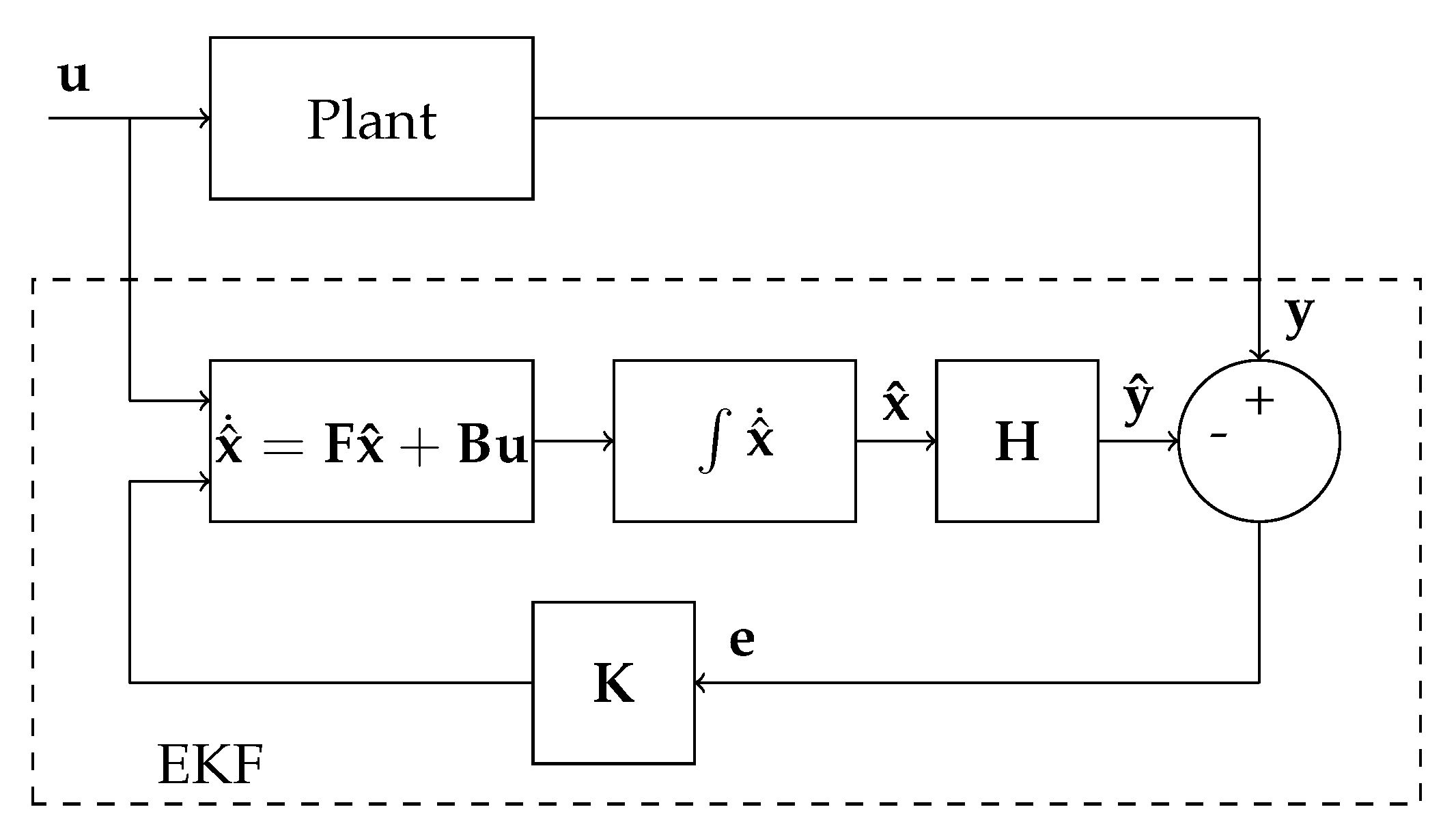
The Kalman filter is a mathematical model that runs in parallel to the actual system and provides the estimation of the states of linear systems. It provides a feedback as the difference between the measured output and constantly corrects the model with the error signal. The feedback gain is calculated so that the estimate of state is optimal. The block diagram of Kalman filter are shown in
Figure 1.
The state-space model for Kalman filter implementation is derived from (
1) with the assumption that the speed
is constant during the switching period [
22,
23].
The
-
axes stator currents
,
, the angular electrical rotor speed
and position
are treated as system states. The voltages
,
as the input variables. A nonlinear dynamic model accounting for the state transition
and measurement noise
can be expressed generally as:
The Gaussian noises
and
are white, zero-mean and uncorrelated, and have known covariance matrices
and
respectively. For good EKF performance the choice of the covariance matrices
,
and
is crucial. The covariance matrices
,
and
are symmetric and positive defined symmetric matrices. Covariance matrices give the statistical description of the model inaccuracy. Matrix
represents the statistical description of the model, matrix
indicates the magnitude of measurement noise, matrix
contains the information of variances at the initial conditions and mainly affects the convergence rate of EKF in the transient condition [
24]. Since these are usually unknown, in most cases the EKF matrices are designed and tuned by trial-and-error procedures [
25].The state vector
is denoted as
is input vector and
is the output vector:
The model’s matrices are expressed as follows:
where
T is sampling time. The PMSM model described by (
6) is nonlinear as products of variables are involved. The nonlinear function
is approximated by a linear set. The continous time Jacobian matrix is expressed as:
where the previous estimate of
as a reference point is taken for discretization around this point. For digital implementation the system model (
4) has to be discretized. The discrete nonlinear dynamic model is expressed as follows:
where in (
11) the matrices
,
,
are discrete matrices of
,
,
respectively, and the matrices
,
are discrete matrices of
,
respectively, independent of the system state. Based on Equation (
9) after discretization of
the Jacobian matrix is:
where the matrix
in (
11) is a discrete, linearized Jacobian matrix.
The extended Kalman filter can be realized by the following steps. The first step is a time update of the state vector and the error covariance matrix, in which a prediction based on the previous estimates
is performed:
where the Jacobian matrix (
12) is computed too. Important to note is that the state prediction is done by integrating Equation (
13) with Runge-Kutta or other similar method. The second step is a measurement update that corrects the predicted state estimate
and its error covariance
matrix through a feedback correction:
where the extended Kalman filter gain matrix
is:
Also the correction of the estimated rotor position (
18) to limit the angle to a
interval is added:
The estimation error covariance matrix
denotes the error of the state vector
(
19).
where
is an operator computing the mean of the variable inside the brackets and
is the mean of the estimated variable. The error covariance matrix
is a degree of accuracy of the estimate. If
is large the error of the estimate is large and if is small the error of the estimate is small. The element
is the variance of the rotor position and it could be an indicator of how well the Kalman filter estimate rotor position. The Kalman gain matrix (
20):
is used as weighting in the measurement update process. The measurement update Equation (
16) corrects the state, accounting for the measurements, and can be expressed as:
In Equation (
21) the elements
and
are position correction gains. As only the stator winding currents can be measured, the rotor position and velocity are mainly estimated in measurement update steps.
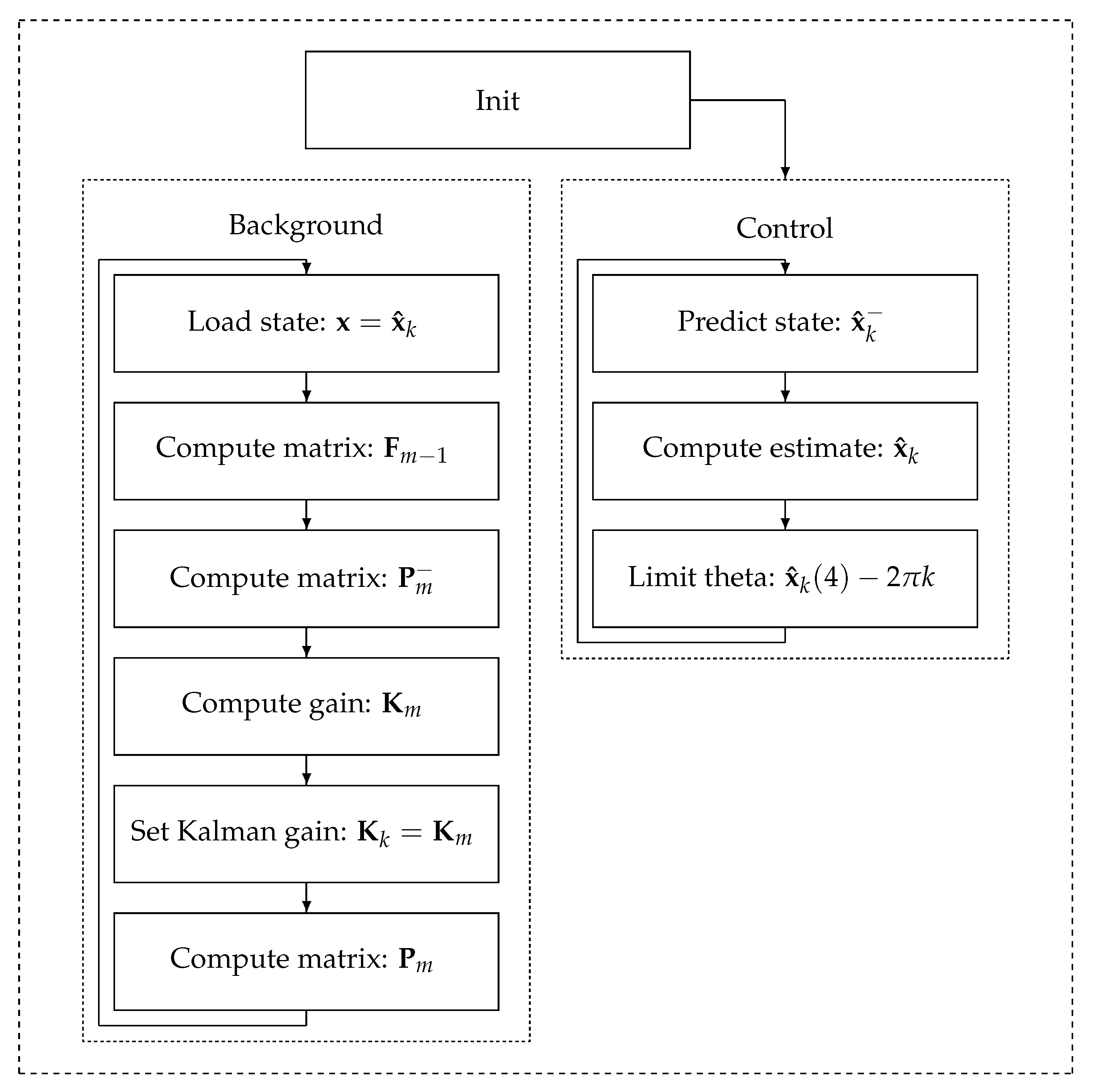
EKF Technique with Parallel Calculation
The EKF calculation is separated into two different procedures. One is the control procedure and the other the background procedure. The sequence of the EKF algorithm implementation is shown in
Figure 2 as a flow diagram.
The control procedure is executed on every PWM switching period and predicts the new state vector using (
13), updates the predicted state vector using (
16). And also corrects the estimated rotor position to a periodic function using (
18). The background procedure calculates the Kalman gain and all covariance matrices. The background is executed on every time
m. The majority of the EKF algorithm computation is performed in the background procedure and runs in a periodic cycle, just like the control procedure. The calling rate of the background procedure is the same or smaller, compared to the control procedure.
The reduced Kalman gain and all covariance matrices calculation ratio could be treated like PMSM model are constant for period of time equal to background procedure call period. While the Kalman gain and all covariance matrices calculation ratio is reduced the prediction state (
13) and measurement correction state (
16) are executed on every control cycle. The prediction state (
13) is always updated with the newest input variables in every control cycle. The measurement correction state (
16) is also fed with the newest measurements, but with the Kalman gains being constant for a period of time equal to control period.
As shown in
Figure 3 the background task period
is longer or the same compared to
where
is PWM switching frequency. The background procedure is separated from the control procedure and does not depend on the PWM switching frequency. The switching frequency can be set to a very high value, while the background procedure can run at a much lower frequency. The total process execution time of EKF could be significantly reduced, because the heavy calculation are doing in background task with period longer than control period.
The control procedure has a higher priority and interrupts the background procedure when it is time to execute it. The synchronization is also performed in the background task, the state vector is taken from the control procedure and the Kalman gain is provided to the control procedure after it is computed. After Kalman gain has been computed in the background procedure, it is important immediately to copy the new Kalman gain matrix into the control procedure to allow control procedure more effectively, to use Kalman gain.
4. Simulation Results
Simulations have been performed with the Matlab programming language. To verify the performance of the proposed EKF algorithm, the simulated PMSM parameters were set for the same values as in the experimental setup and are presented in
Table 1.
In order to make the simulation model consistent with further experimental verification, the space vector pulse width modulation (SVPWM) and overall field oriented control system was simulated. In order to verify the effectiveness of the EKF algorithm based on parallel computation, the simulation was carried out for different set point speed values. The performance of sensorless control for various motor speeds is investigated in simulation. The initial state covariance matrix
and covariance matrices accounting for the model and measurement (
and
respectively) are as follows:
The EKF algorithm in
Figure 2 was the main research object. There, the Kalman gain matrix and its covariance matrices calculation is performed in the background procedure while the prediction and update in the control procedure. The different frequency ratios of the background to the control procedure of the EKF performance at various fundamental motor speeds was researched.
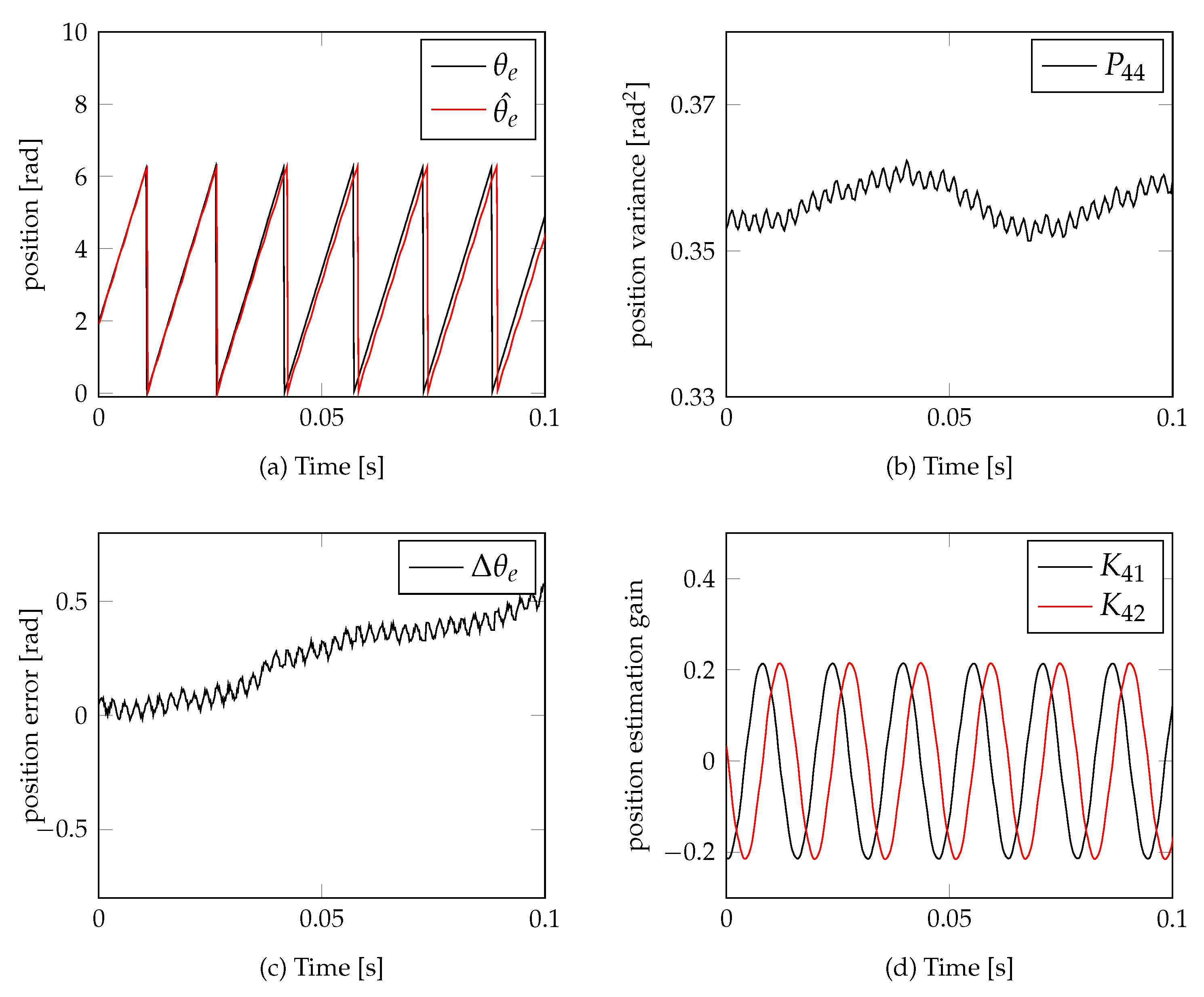
The EKF performance, the Kalman gain and all covariance matrices calculated at the same rate of 5 kHz, are shown in
Figure 4. In
Figure 5 the Kalman gain and all covariance matrices are calculated at a five times slower rate of
1 kHz, while the control procedure execution rate is the same (5 kHz). Comparing
Figure 4c with
Figure 5c can be seen that the position error did not increase. The position variance
in
Figure 4b and
Figure 5b is approximately equal too, only the discretization is different. The Kalman gains
and
for position estimation in
Figure 4d and
Figure 5d have the same amplitude peak values and have similar sine waveform shapes, but the waveform in
Figure 5d are more discretized. The discretization is because of reduced calculation frequency of Kalman gain in simulation is taken. From comparison of
Figure 4 and
Figure 5 we can conclude that the magnitudes of Kalman gain for position estimation did not change, only it’s discretization. For a period of time Kalman gain values are constant values, and they are used multiple time in correction step. Even Kalman gains are constant values the prediction step and correction steps still corrects state vector accounting new measurements.
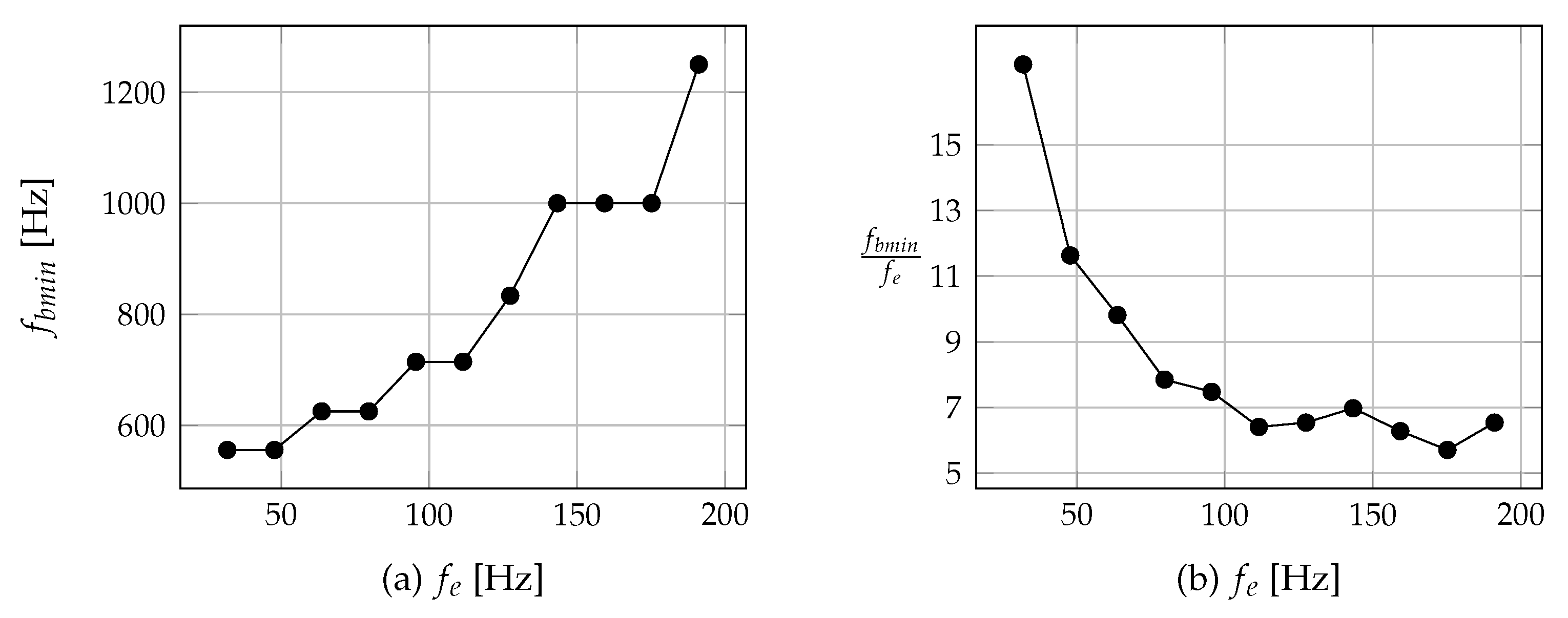
Further simulation has shown, that slowing down the Kalman gain and covariance matrices calculation frequency could cause a rise in the rotor position estimation error, causing a loss of the synchronization and causing the rotor speed to drop to zero. The relation between the minimum Kalman gain and covariance matrices calculation frequency
and the fundamental rotor electrical rotor frequency (
) was investigated. To found the relation
the simulations were run by decreasing frequency
for fixed rotor speed reference set-point
until control was lost. The loss of control was easily determined from rotor speed not able to reach reference speed in simulation. For various rotor reference speeds
the minimum Kalman gain update frequency
are shown in
Figure 6a. From
Figure 6a we can conclude that the higher the reference speed was set the higher Kalman gain update frequency was required. From
Figure 6a we can see linear trend of
to
. The steps in
Figure 6a mainly are due to simulation strategy when frequencie
were selected in steps by dividing switching frequency by integer value (
n, n = 1,2…). The
Figure 6b is obtained from figure
Figure 6a by dividing each
by
. While the data in
Figure 6b are the same we can see how many times we have to compute Kalman gain per rotor electrical frequency without lost control.
5. Implementation
For the implementation of the EKF algorithm in a real experimental drive system an NXP LPC1549 microcontroller was used. The LPC1549 microcontroller is a 32 bit ARM Cortex-M3 based microcontroller operating at a frequency of up to 72 MHz. It is a microcontroller characterized by a low cost and very low power consumption. It includes two 2 Msamples ADCs, four voltage comparators and a PWM/timer subsystem with four configurable multi-purpose state configurable timers. As the LPC1549 microcontroller does not support of floating point operations, all calculation was performed on integer type variables. Data type of the variables used in the implementation is 16 bit fixed point variable with 32 bit long words. For the implementation in C language and code compilation the IAR compiler was used. Different optimization levels for speed comparison are given in
Table 2.
The EKF algorithm implementation using common matrices calculation procedures, with the IAR compiler and with no optimization, gave the longest total execution time 260.4 s. Better results were obtained by setting the compiler optimization to a high level. However, the total execution time is still too long for a practical application. A good execution optimization could be achieved by discarding the common matrices calculation procedures, replacing them with simple arithmetic expressions and accounting for all zero elements and symmetry. In this case the total execution time drops to 37.7 s and could be used for some practical applications.
However, in situations where very high switching frequency is desired, or other heavy calculations need to be performed, the execution time could still be too long. By implementing the EKF algorithm given in
Figure 2 the total execution time could be reduced further. In experimental implementation the switching frequency is selected as 5 kHz and the background procedure call frequency is 1 kHz. In this case the total microcontroller usage for the EKF algorithm calculation is 6.21%. However, if the entire EKF calculation is performed in one switching period, the microcontroller uses as much as is 18.85% of its computational power. With these settings the total microcontroller processing time for EKF is reduced more than 3 times.
6. Experimental Setup and Results
The experimental test platform is shown in
Figure 7. The test setup mainly consists of: a 30 W PMSM motor driven by an NXP inverter FRDM-MC-LVPMSM; other PMSM as a load; the NXP board Xpresso-LPC1549; DC voltage power supply 24V; 360P photoelectric incremental rotary encoder; personal computer (PC).
The PMSM parameters used in experimental setup are defined in
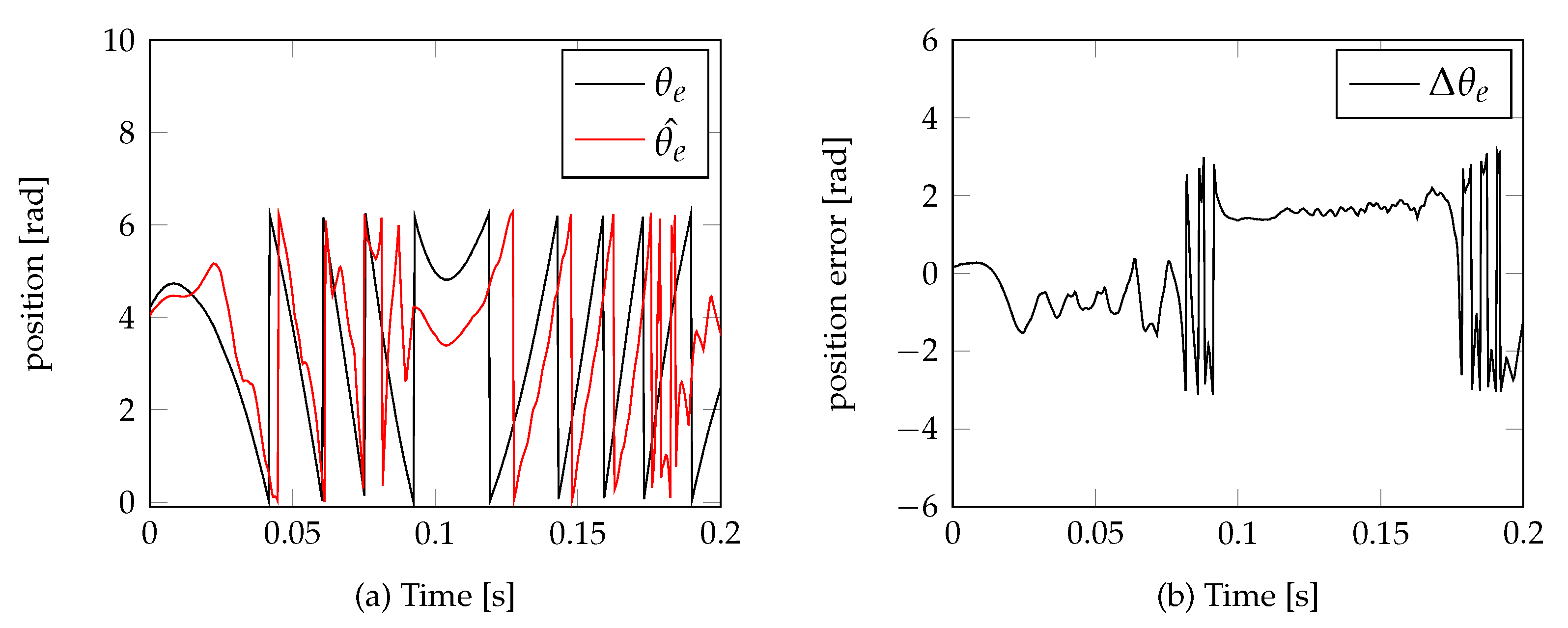
Table 3. All measurements are done in real time by an LPC1549 microcontroller and data are transferred into a personal computer. The phase current was sampled by sensors while the phase voltages taken from control algorithm. The rotor position estimated by the EKF was compared to the signal obtained from a photoelectric incremental rotary encoder. In
Figure 8a the estimated rotor position is compared with rotor position measured by the encoder, for the reference speed set to 400 rad/s.
Figure 8b shows position variance and
Figure 8d presents the Kalman gains for position measurement corrections. The switching frequency
was set for 5 kHz, while the Kalman gain and all covariance matrices are calculated at the same frequency of
5 kHz.
In
Figure 9 the same measurements are performed, but with a reduced Kalman gain and covariance matrices calculation frequency
of 1 kHz. To get results in
Figure 9 the Kalman gain and covariance matrices are computed 5 times slower. Comparing the results presented in
Figure 8b with
Figure 9b one can see, that the position error is about the same average value. More details about position error dependency are presented below. The position variance
in
Figure 8a and
Figure 9a is about the same average value [
]. This means that the variance of estimated position did not change with reduced Kalman gain and covariance matrices calculation frequency. The Kalman gains for position estimation in
Figure 8d and
Figure 9d have the same amplitude peak values and have similar shapes, but the shape in
Figure 9d are more discrete. A bigger discretization steps are mainly due to reduced calculation frequency of Kalman gain. During a short time (
) the Kalman gain matrix is assumed to be a constant value. And the Kalman gain matrix is used multiple times in control procedure until background procedure calculates new one.
Further experimental tests have shown that the position error did not increase when reducing the Kalman gain, and it’s covariance matrices calculation rate, until some minimum frequency
is reached. The position errors at various
frequencies are shown in
Figure 10. In
Figure 10e the Kalman gain, and it’s covariance matrices calculation update rate is 12 times slower (
) than the switching frequency, while the position error order is about the same, as when calculated in every switching instance.
However, slowing the Kalman gain and covariance matrices calculation update rate will cause the synchronization to be lost. By setting:
and reference speed
400 Hz the synchronization is lost, and the rotor speed drops to zero and reverse spin occurs as shown in
Figure 11.
The last experimental tests have shown that the minimum Kalman gain and covariance matrices calculation update rate depends on the fundamental electrical rotor speed and this relation is very similar to simulation results.
The
Figure 12a depicts the relation between the minimum matrices calculation frequency
and fundamental rotor frequency
. To obtain the relation of
the experiments with different speed reference points was analyzed. For each speed reference point, the minimum frequency
was searched. The frequency
considered enough high if the motor speed with constant reference speed was controllable. In the experiment, the frequency
was reduced until the control was lost. The loss of the control was easy to see from the rotor speed not able to follow the speed reference set-point, the speed of the rotor dropped to zero. The synchronization was obviously lost. From this experiments it could be seen that the higher the reference speed, the higher update matrices calculation rate was needed. From
Figure 12a the relation of minimum required
and
is linear. The
Figure 12b presents the same measured data as in
Figure 12a, by taking ratio
. From
Figure 12b can be seen how many times per rotor electrical period, the Kalman gain and covariance matrices has to be computed without losing control. From
Figure 12b we can conclude, that for high frequencies (
Hz) the minimum 7 times Kalman gain and covariance matrices have to be computed per one rotor electrical period. The lower ratio of the Kalman gain and covariance matrices calculation ratio (
) will mostly cause lost control. The higher ratio (
) of course will be good, but the higher ratio means more computation power are needed. Also, from
Figure 12b we can conclude, that at low frequencies (
Hz) the ratio
is higher than 7 is needed, but from
Figure 12a we can see that the required minimum frequency
is decreasing even if the ratio increase
.
ARM Cortex-M3 LPC1549 processor usages for executing EKF estimator with various background frequencies are given in
Table 4. The data from
Table 2 was used for calculating usages. Also, by applying the role that at least 7 times per one rotor electrical period Kalman gain and covariance matrices have to be computed, we get maximum allowed electrical frequency (
) in control. That level of optimization to choose is a trade-off decision between processor usage and the maximum allowed electrical frequency in the system.
From
Table 4 can be seen that even reduction of background frequency by two times from 5 kHz to 2.5 kHz gives a good time optimization. The further reduction gives less win of the processor time for each step.


