Abstract
Since the affirming of global warming, most wind energy projects have focused on the large-scale Horizontal Axis Wind Turbines (HAWTs). In recent years, the fast-growing wind energy sector and the demand for smarter grids have led to the use of Vertical Axis Wind Turbines (VAWTs) for decentralized energy generation systems, both in urban and remote rural areas. The goals of this study are to improve the Savonius-type VAWT’s efficiency and oscillation. The main concept is to redesign a Novel Blade profile using the Taguchi Robust Design Method and the ANSYS-Fluent simulation package. The convex contour of the blade faces against the wind, creating sufficient lift force and minimizing drag force; the concave contour faces up to the wind, improving or maintaining the drag force. The result is that the Novel Blade improves blade performance by 65% over the Savonius type at the best angular position. In addition, it decreases the oscillation and noise accordingly. This study achieved its two goals.
1. Introduction
In 2010, the United Nations affirmed that global warming is caused mainly by carbon dioxide , emitted mostly from fossil fuels. Severe global climate changes are now believed to be the most significant environmental threat to the earth and to human beings. There has been a global push for renewable energy and zero CO2 emissions, which is generally called “Green” energy; this energy includes hydraulic, thermal, solar, and wind energy, among others. Most of those energies must be transformed into “Electricity” and stored or transmitted before usage. The wind energy system is one of the most cost-effective and fast-growing systems among the currently exploited green and renewable energy sources. As a result, wind power generation systems have seen increasing investment and improved efficiency over the last decades.
The wind turbine generating system has two basic categories: Vertical Axis Wind Turbines (VAWTs) and Horizontal Axis Wind Turbines (HAWTs). The efficiency of VAWTs is generally in the range of 15–20%, which is less than half of the HAWT efficiency. The main reason is that only half of the VAWT sliding area can create a productive driving force. In addition, the VAWT’s constant changes in the angle of attack (AOA) during the rotating cycle causes flow separation, dynamic stall, and imbalanced driving force onto two sides of the rotor. This subsequently results in significant instability of aerodynamic performance and induces oscillation and noises [1,2]. This is why the VAWT has long been ignored and devalued. However, the VAWT has certain natural advantages over the HAWT, such as its simple mechanism, easy maintenance, simple structure, low cost, and lack of yawing. The VAWT has become more popular in recent years and will play a leading role in future wind power [3,4], especially for smarter grids with decentralized wind energy generation systems located in urban and remote rural areas, where the wind can be very turbulent and unsteady [5,6,7].
The modern VAWT has evolved into three basic types: Savonius [8,9], Darrieus [10,11], and H-rotor [12]. Darrieus and H-rotor are lift-type VAWTs. At the still position, the lift-type blades generate insufficient lift forces or minor drag forces only, which results in an inability to self-start. This is a serious disadvantage of the lift-type VAWT. The Savonius type is the iconic drag type and the pioneer model of the VAWT. Both the concave and convex profiles of the blade generate drag forces, but in the opposite direction of spinning. This is the reason that the efficiency of the Savonius type is lower than the lift type. Nevertheless, the Savonius-type VAWT has many advantages over the lift type, such as its compact scale, excellent self-starting, low cost, low rotation speed, and low noise emission [9,13]. Moreover, there is no severe restriction for the blade material, and the manufacture of the Savonius turbine for power generation is easy to realize on-site [14,15]. Therefore, the Savonius-type VAWT has been developed widely up to now.
The efficiency of the wind turbine generating system is related to the generator performance, turbine rotor, and blade profile as well as the compatibility of these three elements. Aerodynamically, the wind blowing over and onto a wind blade will create a lift force and drag force. The primary goal is to improve the efficiency of the Savonius-type VAWT by focusing on redesigning a Novel Blade profile. The secondary goal is to minimize the disparity between the drag force on the concave contour and the lift force on the convex contour; this is the key factor related to oscillation and noise.
The novelties of the optimal design of drag-type blades are as follows: (1) On the convex contour of the wind blades, the focus is not only to reduce the drag force but also to generate maximum lift force to pull the blades forward. (2) On the concave contour of the blade, the focus is to extract more drag force to push the blade backward. There are few studies on increasing the lift force on the convex contour; research is generally focused only on increasing drag force on the concave contour. By solely focusing on the latter, it is impossible to improve the overall efficiency and reduce the oscillation and noise issues of the Savonius-type VAWT.
First, we identify the control factors with different levels of the drag-type blade profile, then we perform the Taguchi Method to format the orthogonal array table to list the required combinations for simulations. This facilitates initial analysis of possible designs with sufficient accuracy and saves abundant computational resources at the design stage. Then, we use the ANSYS-Fluent simulation software to simulate each possible blade profile combination for obtaining detailed transient analysis and the flow line distribution. Finally, we compare, analyze, and verify the derived simulation data.
This paper is composed as follows: Section 1, the Introduction, presents the background of this study. Section 2, the methodology, presents the method of designing and modeling the novel blade profile. Section 3, the modeling, addresses the Taguchi Method to identify each parameter of the optimal blade profile and then details the ANSYS-Fluent used to simulate the lift coefficient (Cl) on the convex contour and the drag coefficient (Cd) on the concave contour. Section 4, the results, presents the final optimal blade geometry with several considerations, and Section 5 outlines conclusions and recommendations.
2. Methodology
The methodology used in this study is described in four sections. Section 2.1—Why and How—lists basic knowledge and theories relevant to aerodynamics and wind turbines. It brings forth the ideas of why and how to improve the efficiency of the Savonius-type VAWT. Section 2.2—Taguchi Robust Design Method—examines the usage of the Taguchi Method as a robust design framework for the optimal solution and for saving necessary resources. Section 2.3—ANSYS-fluent Meshing—describes the workflow and parameter settings. Section 2.4—ANSYS-fluent Simulation—outlines the workflow and parameter settings.
2.1. Why and How
The wind rotor efficiency depends on the blade geometry, the number of blades, and blade positioning. Although the drag force is greater than the lift force in aerodynamics, the efficiency of the Savonius-type VAWT is far lower than the lift type. The main reason is that it extracts only half of the wind energy for positive work, and the other half is for negative work. While the concave side faces against the wind, it produces the major drag force pushing the rotor spinning positively. While the blades turn 180°, the convex side faces upwind and creates some drag force pushing the rotor spinning reversely.
There are several papers related to the performance improvement of the Savonius VAWT. Some blocked one side of the rotor—the convex side—and diverted the wind energy to the concave side [16,17,18,19]. Some changed the number of Savonius half-cylindrical blades [20] or built a wind tower [21]. Some merely modified the contour of the wind blades for increasing drag coefficient only, using blades such as spline-type and Bach-type blades [22,23], elliptical blades [24], and twisted blades [25]. Most of these improved efficiency of the drag force on the concave side of the blade only. This also entailed certain disadvantages, such as complex structure, increased cost, and more oscillation.
The choice of a wind machine is based on the energetic performance of the rotor blade. The equations of lift force and drag force use the same equation but with a different coefficient (drag/lift), as specified in Equation (1).
where F = force (drag/lift); ρ = air density; ν = wind velocity; C = coefficient (drag/lift); A = the reference area.
Increasing the reference area is simple, and can be done solely by enlarging the blade size as long as the stress and structure can sustain its weight. Increasing the coefficient is much more complicated and involves the design of blade geometry and positioning. The value of the drag/lift coefficient is not calculated but measured. It is not an absolute constant figure. It varies with the blade geometry and wind velocity and more generally with Reynolds number (Re). In this study, the drag coefficient of various three-dimensional blade geometries, measured at Re number between and, is specified in Figure 1 [26].
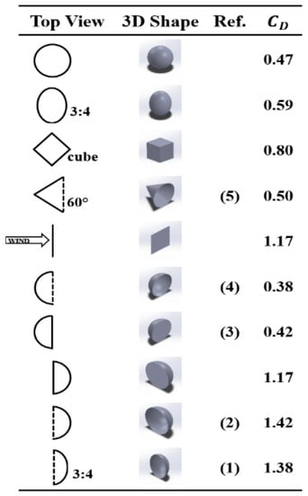
Figure 1.
Referenced drag coefficients.
Based on aerodynamic theories and equations, relevant references of lift and drag characteristics, and empirical principles, the preliminary conceptual design of the Novel Blade geometry was composed. The main framework is used to create sufficient lift coefficient and to reduce the drag coefficient on the convex contour. At the same time, it must not lose any of the drag coefficient on the concave profile. It also must minimize the disparity value and the drag force on the concave contour versus the lift force on the convex, for reducing oscillation and noise.
As per Ref. (1) and (2) in Figure 1, where referenced drag coefficients show longer hollowed blade shapes, the drag coefficient increases. Therefore, the concave side of the novel blade may curve inward deeper to some extent. As per Ref. (3), (4), and (5) in Figure 1, a sharper and smoother shape has a lower drag coefficient; the acute angle, oval shape, and rounded shape may be considered as the apex of the convex profile. In addition, it is covered with the shelters on both the top and bottom sides of the novel blade body. It covers the inside edge of the blade body and may maintain the wind energy inside the concave contour rather than flowing out of it. It improves the positive drag forces but must not exceed Betz Limits: 59.3% kinetic energy of the wind. The shelter that spreads outside of the blade edge works as the winglet of an airplane. It may guide the wind stream smoothly, flowing along the blade surfaces, and eliminate the eddy current at the edge of the blade body. This may increase more lift forces and reduce the drag forces onto the convex contour. The design of the conceptual geometry is illustrated in Figure 3.
2.2. Taguchi Robust Design Methods
There are many different algorithms for optimizing VAWT efficiencies, such as artificial neural networks and genetic algorithms [27]. This study chooses the Taguchi Methods of Robust Design, an engineering methodology for improving productivity at the research and development stage. It provides high-quality solutions quickly and at a lower cost. The robust design draws on many ideas, from statistical experimental design to planning experiments for obtaining reliable information about the variables involved in making engineering decisions. The Taguchi Methods of Robust Design use two primary implements. The first one is the orthogonal array, which studies multiple design parameters simultaneously; the second one is the signal-to-noise (S/N) ratio, which measures the quality value. The methods have been used in virtually all engineering fields and business applications. As to the loss functions, the Taguchi Methods specify the three characteristics of larger the better, smaller the better, and nominal the better. In this study, the purpose is to maximize both the drag coefficient and lift coefficient of the blade. Therefore, this study uses the characteristic of larger the better and lists its equation of S/N ratio as Equation (2):
where S/N = Signal/Noise Ratio; y = Coefficient (measured value).
In the study, the steps of executing the Taguchi Methods are summarized as follows:
- Identify four control factors, each with three alternative levels according to relevant engineering knowledge for designing the novel rotor blade.
- Design the matrix combinations as an orthogonal array of L9(34) for the required experiments for studying the effect of four control factors and three levels simultaneously.
- Simulate each combination in the matrix of the orthogonal array by using the ANSYS-Fluent, and log simulation data into the orthogonal array table.
- Analyze the simulation data, through the large the better equation of the S/N ratio, to calculate the optimum levels for the control factors and predict performance under these levels.
- Conduct the verification experiment for the best combination, with each control factor having the optimum level derived from matrix experiments.
2.3. ANSYS-Fluent Meshing
The ANSYS-Fluent has built-in meshing capability that creates the exhaustive mesh and troubleshoots mesh connectivity within the same workflow. Therefore, the grid generation in the study is obtained by setting at the default value all required parameters of volume settings, including local sizing, surface meshing, volume mesh, boundary layers, and growth rate. As for checking the mesh quality metrics, the number of nodes and cells, the skewness, and the aspect ratio are calculated automatically and indicated on the console. The y+ is derived from the Plot of the Result for each simulation. The details are listed in Mesh #1 of Table 1, as follows.

Table 1.
Mesh quality parameter table.
The mesh independence study recommended selecting three significantly different sets of grids with geometrically similar cells and running simulations to determine the values of required variables important to the objective of the simulation study [28]. This study performed three more simulations according to the recommendations of increasing the cell number as indicated in Mesh #2, Mesh #3, and Mesh #4 of Table 1, as above. The comparison of the three simulation Cd results shows only a slight variance, with all within one percent.
2.4. ANSYS-Fluent Simulation
The ANSYS-Fluent is a general-purpose software package for simulating interactions with physics, structure, vibration, fluid dynamics, heat transfer, and electromagnetics for engineers. The setting of the ANSYS-Fluent solver has the default of the Pressure-Based Type, Absolute Velocity Formulation, and Steady Time Step. The governing equations of the fluid flow model considered in the study are the incompressible Reynolds-averaged Naiver–Stokes equations (RANS) coupled with the one-equation Spalart-Allmaras model (SA), a low-cost RANS model solving a transport equation for a modified eddy viscosity for aerospace applications involving wall-bounded flows that has given good results for boundary layers subjected to adverse pressure gradients. Adopting the standard SA model, the complete set of governing equations (Equations (3)–(5)) are as follows:
where:
The SIMPLE (Semi Implicit Method for Pressure Linked Equations) algorithm was chosen to solve the conservation equations via pressure correction because of its computing efficiency, robust iteration for coupling parameters, and high-order differencing schemes. The second-order upwind interpolating scheme was used for all the equations and applied the first-order implicit for transient formulation. This second-order algorithm is capable of reducing interpolation errors and computing correct numerical diffusion. The inlet wind speed of boundary condition is 3 m/s. The equation residual value was at a setting of 1 × 10⁻⁵, and all simulations converged to a residual of 1 × 10⁻⁹. The solution method is the coupled scheme and second-order upwind turbulent viscosity, the solution initialization is the hybrid method, and the run calculation is 300 iterations. The other parameters are all in default as recommended by ANSYS-Fluent.
3. Modeling Method
For easy referencing, the modeling process flows for both the Taguchi Methods and the ANSYS-Fluent are illustrated step by step in Figure 2, the Diagram of Modeling Process Flow.
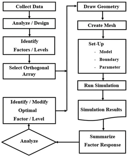
Figure 2.
Diagram of modeling process flow.
Based on the conceptual design and understanding, the dimensions and geometries of the novel blade model are as follows: on the concave profile, the setting of the reference area is 120 mm width and 120 mm height, then curve inward 110, 120, and 130 mm in depth. On the convex profile, the apex contours are designed in the acute angle and oval shape and are rounded in three different contours. At the top and bottom shelters of the blade, winglets with 5, 10, and 15 mm in width are spread to the outside blade edge, then covered with 1/3, 2/3, and full-size shelter to the inside blade edge. For easy referencing, the conceptual dimensions and geometries of the Novel Blade profile are illustrated in Figure 3 below, which includes three diagrams of rotating direction as well as front- and back-view diagrams as the concave and convex contours, respectively.
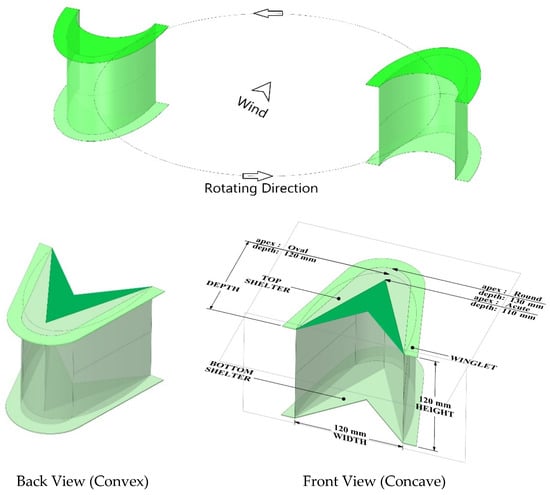
Figure 3.
Conceptual design of Novel Blade profile.
As illustrated in Figure 3, there are four control factors, each with three levels, as specified in Table 2 below.
Table 2.
Control factors and levels.
As per Table 2, the matrix combination is formed according to the Taguchi method designated for four control factors with three levels each, namely the L9 (34) orthogonal array as specified Table 3 below. The L9 (34) also means that only nine experiments are required instead of 81 of each possible combination. That saves a vast amount of effort, resources, time, and cost.
Table 3.
L9 (34) orthogonal array.
First, for simulating the concave contour, it is positioned against the direction of wind velocity. Then, nine combinations of the concave profiles are simulated using the ANSYS-Fluent, as shown in Table 3, and nine sets of Cd data are derived. The purpose of this study is to create optimal drag force on the concave side. It calculates Cd data with the characteristic of the larger the better for the S/N ratio. Finally, each set of derived Cd data and S/N ratio is logged in the columns of Y and S/N (Table 4 below), respectively.
Table 4.
Concave ANSYS simulation data.
In the next step, the S/N ratio is analyzed for identifying the optimum levels for each control factor of concave contour and predicting performance under these levels. From the nine experiment results listed in Table 4, three sets of the S/N ratio are excerpted for each control factor with three different levels and then averaged and formed into the matrix in Table 5 below.
Table 5.
Concave S/N ratio for factors/levels.
As per Table 5, the average value of S/N ratio is excerpted for all factors at each level and put it into Table 6 accordingly. Table 6 identifies the best combination of factors with the best level as A2-B2-C3-D1.
Table 6.
Concave factor/level response.
For drag-type rotor blades, both concave and convex sides would be facing upfront to the wind blow direction alternately. Therefore, it is necessary to perform simulation on both sides of the blade. The simulation of the convex contour requires an angle of attack (AOA) toward the wind velocity to produce the lift force. This study positions the blades at 20° of AOA because the AOA for many airfoils is typically around 15°–20°.
For the convex contour simulation, the blades are turned to 20° in the direction of the wind velocity. Then, nine experiments are conducted using ANSYS-Fluent to simulate nine convex profiles with different combinations, as shown in Table 3, and derive nine sets of Cι data. The purpose of this study is to create optimal lift force on the convex side. Therefore, Cι data is calculated for the S/N ratio with the characteristic of the larger the better. Finally, each derived set of Cι data and S/N ratio is logged into the columns of Y and S/N, respectively, in Table 7.
Table 7.
Convex ANSYS simulation data.
In the next step, the S/N ratio is analyzed to identify the optimum levels for each control factor of the convex contour and to predict performance under these levels. From the nine experiment results listed in Table 7, three sets of the S/N ratio are excerpted for each control factor with three different levels and are averaged to form the matrix in Table 8, below.
Table 8.
Convex S/N Ratio for factors/levels.
As per Table 8, the average value of S/N ratio for the factors and each level is excerpted and put it into Table 9, below. Table 9 identifies the best combination of factors with the best level as A2-B3-C3-D3.
Table 9.
Convex factors/level response.
4. Results and Discussion
- Factor/Level A2 and C3 are consistent for both the concave and convex contour.
- Factor/Level A2 oval shape is the best for the apex.
- The B3 for Factor B, Blade Depth, is recommended, regardless of the fact that in Table 6 the best factor/level on the concave surface is B2. This is because the S/N ratio loss between B2 and B3 is slight when comparing the loss on the concave contour to the convex.
- For the Factor/Level C3, Winglet, the results show that a wider winglet is better. Therefore, we recommend enlarging from C3 = 15 mm to C4 = 20 mm. This may extend farther as long as the structure can tolerate it.
- For the Factor D, Shelter, we adopted both Level 1 and 3 as Combination #1 A2-B3-C4-D1 and Combination #2 A2-B3-C4-D3, respectively, as expressed in Table 10. The simulation results show the optimal shelter coverage should be between 1/3 and 2/3. Therefore, the Level is adjusted to 4, 1/2 Shelter, and expressed as Combination #3 A2-B3-C4-D4 in Table 10.
Table 10. Analysis results summary.
- For increasing the drag/lift coefficient, the height of Combination #3 is elongated from 120 to 140 mm, expressed by Ex, becoming the Novel Blade indicated as A2-B3-C4-D4-Ex in Table 10 and pictured as Figure 4 below.
 Figure 4. Novel Blade profile: A2-B3-C4-D4-Ex.
 - For comparison, the semi-circular Savonius type is set with the same reference area, 140 mm * 120 mm, without the Factor C, Winglet, and Factor D, Shelter, and expressed as A3-B0-Co-Do-Ex in Table 10 and pictured as Figure 5 below.
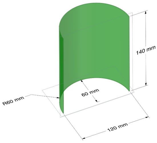 Figure 5. Savonius blade profile: A3-B0-Co-Do-Ex.
Table 10 shows that on the convex profile, the Novel Blade lift coefficient (0.1298) is much higher than the Savonius-type (0.0354), and the drag coefficient is about the same, 0.1128 vs. 0.1115, respectively. As to the drag coefficient on the concave profile, the Novel Blade shows some improvement over the Savonius type: 0.2361 vs. 0.2293, respectively. The total drag/lift coefficient for the positive work is the sum of concave Cd, the convex Cl, and the convex Cd, for which the Novel Blade value is 0.2531 and the Savonius type value is 0.1532. The total drag force is the sum of both sides’ drag coefficients, and the lift force is the lift coefficient on the convex contour only, as there is no lift coefficient on the concave profile. The total drag coefficient for the Novel Blade and the Savonius type is 0.1233 and 0.1178, respectively.
For visual comparison of the above numerical simulation and comparison, the pressure distribution diagram confirms that the pressure force on the concave contour of the Novel Blade is greater than on the Savonius type, about 6.13 vs. 5.32 (pascal), respectively, as illustrated in Figure 6. This means that the Novel Blade will produce more drag force. The diagram of streamlines flew over the convex contour, indicating that the flow lines on the Novel Blade are much longer and denser than the Savonius-type, as illustrated in Figure 7. This means that the novel blade will create more lift force.
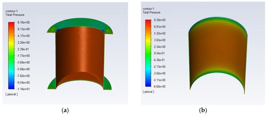
Figure 6.
Pressure on concave contour: (a) Novel Blade geometry; (b) Savonius-type blade.
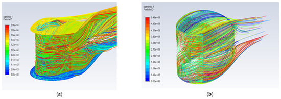
Figure 7.
Stream lines on convex contour: (a) Novel Blade geometry; (b) Savonius-type blade.
5. Conclusions
In this study, the blades were simulated at the best angular position for the drag force concave profile facing upfront to the wind and for the lift force convex contour facing against the wind at an AOA of 20 degrees. Although the simulation results showed the best angular position only, they could still show the tendencies of the characteristics of the wind blades.
In summary, it is startling that the total drag/lift coefficient for the positive works increases by over 65% (0.2531 vs. 0.1532), which means that the Novel Blade improves blade performance over the Savonius type by 65% at the best angular position.
The disparity value is an imbalanced driving force on the two sides of the rotating rotor, which is the difference between the total drag force on the concave contour and the lift force on the convex profile. The disparity values of the Novel Blade and Savonius type are 0.0065 (0.1298–0.1233) and 0.0824 (0.1178–0.0345), respectively. The disparity of the Novel Blade reduced by 93% (0.0065 vs. 0.0824) compared to the Savonius type, which means the Novel Blade improves the instability of aerodynamic performance and decreases oscillation and noises accordingly.
In conclusion of this study, it achieved its two goals. The results are promising, as both design tools used coincided with each other sufficiently. This study confirmed the future possibilities of the Novel Blade as a Savonius-type VAWT.
In the process of study, we explored many ideas and questions. There are recommendations on two themes: (1) further fine-tuning the winglet width and coverage area of shelter using the same methodology as this study; (2) building a full-scale Novel Blade and mounting it on a wind rotor, then testing it in a wind tunnel for verifying the improvement of the wind rotor performance.
Author Contributions
Primary author of this paper, T.-L.C.; supervision and support, S.-F.T. and C.-L.C.; academic and technical research, T.-L.C. All authors have read and agreed to the published version of the manuscript.
Funding
This research was funded by the Ministry of Science and Technology, Taiwan, under grants MOST 107-2218-E-002-068.
Acknowledgments
The authors would like to thank the Marine Engineering Department of National Taiwan Ocean University for supporting this research. The authors are also grateful to those professors and graduate students who provided their valuable comments and suggestions for this paper. Especially the funding from the Ministry of Science and Technology, Taiwan, under grants MOST 107-2218-E-002-068.
Conflicts of Interest
The authors declare no conflict of interest.
References
- Ferreira, C.S.; Van Kuik, G.; Van Bussel, G.; Scarano, F. Visualization by PIV of dynamic stall on a vertical axis wind turbine. Exp. Fluids 2009, 46, 97–108. [Google Scholar] [CrossRef]
- Carr, L.W. Progress in analysis and prediction of dynamic stall. J. Aircr. 1988, 25, 6–17. [Google Scholar] [CrossRef]
- Danao, L.A.; Eboibi, O.; Howell, R. An experimental investigation into the influence of unsteady wind on the performance of a vertical axis wind turbine. Appl. Energy 2013, 107, 403–411. [Google Scholar] [CrossRef]
- Eriksson, S.; Bernhoff, H.; Leijon, M. Evaluation of different turbine concepts for wind power. Renew. Sustain. Energy Rev. 2008, 12, 1419–1434. [Google Scholar] [CrossRef]
- Mălăel, I.; Dumitrescu, H.; CardoÅŸ, V. Numerical simulation of vertical axis wind turbine at low speed ratios. Glob. J. Res. Eng. 2014, 14, 9–20. [Google Scholar]
- Batista, N.C.; Melício, R.; Matias, J.C.O.; Catalão, J.P.S. Self-start performance evaluation in Darrieus-type vertical axis wind turbines: Methodology and computational tool applied to symmetrical airfoils. ICREPQ’11 2011, 51. [Google Scholar] [CrossRef]
- Zhang, X. Analysis and Optimization of a Novel Wind Turbine. Ph.D. Thesis, University of Hertfordshire, Hertfordshire, UK, 31 January 2014. [Google Scholar]
- D’Alessandro, V.; Montelpare, S.; Ricci, R.; Secchiaroli, A. Unsteady Aerodynamics of a Savonius wind rotor: A new computational approach for the simulation of energy performance. Energy 2010, 35, 3349–3363. [Google Scholar] [CrossRef]
- Shigetomi, A.; Murai, Y.; Tasaka, Y.; Takeda, Y. Interactive flow field around two Savonius turbines. Renew. Energy 2011, 36, 536–545. [Google Scholar] [CrossRef]
- Hill, N.; Dominy, R.; Ingram, G.; Dominy, J. Darrieus turbines: The physics of self-starting. Proc. Inst. Mech. Eng. Part A J. Power Energy 2009, 223, 21–29. [Google Scholar] [CrossRef]
- Castelli, M.R.; Englaro, A.; Benini, E. The Darrieus wind turbine: Proposal for a new performance prediction model based on CFD. Energy 2011, 36, 4919–4934. [Google Scholar] [CrossRef]
- Kjellin, J.; Bülow, F.; Eriksson, S.; Deglaire, P.; Leijon, M.; Bernhoff, H. Power coefficient measurement on a 12 kW straight bladed vertical axis wind turbine. Renew. Energy 2011, 36, 3050–3053. [Google Scholar] [CrossRef]
- Gupta, R.; Biswas, A.; Sharma, K.K. Comparative study of a three-bucket Savonius rotor with a combined three-bucket Savonius–three-bladed Darrieus rotor. Renew. Energy 2008, 33, 1974–1981. [Google Scholar] [CrossRef]
- Valdes, L.C.; Raniriharinosy, K. Low technical wind pumping of high efficiency. Renew. Energy 2001, 24, 275–301. [Google Scholar] [CrossRef]
- Valdès, L.C.; Darque, J. Design of wind-driven generator made up of dynamos assembling. Renew. Energy 2003, 28, 345–362. [Google Scholar] [CrossRef]
- Irabu, K.; Roy, J.N. Characteristics of wind power on Savonius rotor using a guide-box tunnel. Exp. Therm. Fluid Sci. 2007, 32, 580–586. [Google Scholar] [CrossRef]
- Altan, B.D.; Atılgan, M.; Özdamar, A. An experimental study on improvement of a Savonius rotor performance with curtaining. Exp. Therm. Fluid Sci. 2008, 32, 1673–1678. [Google Scholar] [CrossRef]
- Golecha, K.; Eldho, T.I.; Prabhu, S.V. Influence of the deflector plate on the performance of modified Savonius water turbine. Appl. Energy 2011, 88, 3207–3217. [Google Scholar] [CrossRef]
- Altan, B.D.; Atılgan, M. An experimental and numerical study on the improvement of the performance of Savonius wind rotor. Energy Convers. Manag. 2008, 49, 3425–3432. [Google Scholar] [CrossRef]
- Sheldahl, R.E.; Blackwell, B.F.; Feltz, L.V. Wind tunnel performance data for two-and three-bucket Savonius rotors. J. Energy 1978, 2, 160–164. [Google Scholar] [CrossRef]
- Cho, S.Y.; Choi, S.K.; Kim, J.G.; Cho, C.H. Numerical study to investigate the design parameters of a wind tower to improve the performance of a vertical-axis wind turbine. Adv. Mech. Eng. 2017, 9, 1687814017744474. [Google Scholar] [CrossRef]
- Kamoji, M.A.; Kedare, S.B.; Prabhu, S.V. Experimental investigations on single stage modified Savonius rotor. Appl. Energy 2009, 86, 1064–1073. [Google Scholar] [CrossRef]
- Kacprzak, K.; Liskiewicz, G.; Sobczak, K. Numerical investigation of conventional and modified Savonius wind turbines. Renew. Energy 2013, 60, 578–585. [Google Scholar] [CrossRef]
- Tian, W.; Song, B.; Mao, Z. Numerical investigation of a Savonius wind turbine with elliptical blades. Proc. CSEE 2014, 34, 5796–5802. [Google Scholar]
- Saha, U.K.; Rajkumar, M.J. On the performance analysis of Savonius rotor with twisted blades. Renew. Energy 2006, 31, 1776–1788. [Google Scholar] [CrossRef]
- Hoerner, S.F. The table of various shapes’ drag coefficients. In Fluid Dynamic Drag; 1965; pp. 3–17. Available online: http://ftp.demec.ufpr.br/disciplinas/TM240/Marchi/Bibliografia/Hoerner.pdf (accessed on 10 June 2021).
- Svorcan, J.; Peković, O.; Simonović, A.; Tanović, D.; Hasan, M.S. Design of optimal flow concentrator for vertical-axis wind turbines using computational fluid dynamics, artificial neural networks and genetic algorithm. Adv. Mech. Eng. 2021, 13, 16878140211009009. [Google Scholar] [CrossRef]
- Celik, I.B.; Ghia, U.; Roache, P.J.; Freitas, C.J. Procedure for estimation and reporting of uncertainty due to discretization in CFD applications. J. Fluids Eng. Trans. ASME 2008, 130, 078001-1. [Google Scholar]
Publisher’s Note: MDPI stays neutral with regard to jurisdictional claims in published maps and institutional affiliations. |
© 2021 by the authors. Licensee MDPI, Basel, Switzerland. This article is an open access article distributed under the terms and conditions of the Creative Commons Attribution (CC BY) license (https://creativecommons.org/licenses/by/4.0/).