Article

Modeling Sea Ice Effects for Wave Energy Resource Assessments

1
Pacific Northwest National Laboratory, Coastal Sciences Division, Seattle, WA 98109, USA
2
Department of Civil and Environmental Engineering, University of Washington, Seattle, WA 98195, USA
3
Applied Physics Laboratory, University of Washington, Seattle, WA 98105, USA
*
Author to whom correspondence should be addressed.
Energies 2021, 14(12), 3482; https://doi.org/10.3390/en14123482
Submission received: 20 May 2021 / Revised: 5 June 2021 / Accepted: 7 June 2021 / Published: 11 June 2021
(This article belongs to the Special Issue Nearshore Wind and Wave Energy Potential)

Abstract

:
Wave-generated power has potential as a valuable coastal resource, but the wave climate needs to be mapped for feasibility before wave energy converters are installed. Numerical models are used for wave resource assessments to quantify the amount of available power and its seasonality. Alaska is the U.S. state with the longest coastline and has extensive wave resources, but it is affected by seasonal sea ice that dampens the wave energy and the full extent of this dampening is unknown. To accurately characterize the wave resource in regions that experience seasonal sea ice, coastal wave models must account for these effects. The aim of this study is to determine how the dampening effects of sea ice change wave energy resource assessments in the nearshore. Here, we show that by combining high-resolution sea ice imagery with a sea ice/wave dampening parameterization in an unstructured grid, the Simulating Waves Nearshore (SWAN) model improves wave height predictions and demonstrates the extent to which wave power decreases when sea ice is present. The sea ice parametrization decreases the bias and root mean square errors of wave height comparisons with two wave buoys and predicts a decrease in the wave power of up to 100 kW/m in areas around Prince William Sound, Alaska. The magnitude of the improvement of the model/buoy comparison depends on the coefficients used to parameterize the wave–ice interaction.

1. Introduction

Wave energy conversion is an emerging source of renewable energy that has the potential to supply one quarter of the total U.S. annual electricity demand [1]. Alaska has the longest coastline of the 50 U.S. states and sizable waves whose energy could be captured with wave energy converters. The southern Alaskan coastline has been identified as a coastline with potential for wave energy power generation due to the size of the waves and their spectral and directional characteristics [2,3]. A 32-year numerical modeling resource characterization study confirmed the wave energy potential of the southern Alaskan coastline [3] but did not assess the resource in areas with known seasonal sea ice. To accurately assess these regions, numerical models must include the dampening effects of sea ice on the waves that may decrease the available power.
The dampening effects of sea ice on waves have been observed in field campaigns in both the Arctic and Antarctic and the observations have been used to parameterize the ice/wave interactions [4,5,6,7,8,9,10]. The parameterization of the dampening is an active area of research with the dependence on ice type and distance from the ice edge being investigated [11]. Large-scale numerical models have begun to add ice/wave parameterizations to examine the relationship between ocean waves and sea ice [7,9,10,12,13]. This study applies an ice/wave parameterization to waves in nearshore ice along the Alaskan coastline to determine how wave energy resource assessments are affected by the presence of sea ice.
Sea ice occurs seasonally along the Alaskan coastline. In early spring, sea ice is found along most of the coastline (Figure 1a), but by early summer, significant amounts only remain in the north (Figure 1b). In fall, there are no areas with ice coverage (Figure 1c) and by mid-December, ice has been returning to most of the coastline (Figure 1d). The coastline along the northern Gulf of Alaska is a region that has both a very energetic sea state [2] and seasonal sea ice. Prince William Sound (PWS), along the northern Gulf of Alaska, has seasonal sea ice and two wave buoys maintained by the National Data Buoy Center (NDBC), which make it a good site to study the effects of sea ice on the wave energy resource (Figure 2a). Data from a previously published wave model at this location [14] show that the modeled wave heights are overestimated when sea ice is present (Figure 2b).
Wave resource assessments that conform to international standards, such as International Electrotechnical Commission (IEC) TS 62600-101, require consideration of the effect of sea ice. One of the most widely used numerical models for wave resource assessment is the Simulating Waves Nearshore (SWAN) model [3,14,15,16,17,18]; yet, until recently, SWAN has not included the effects of sea ice on waves. With the release of version 41.31, a wave–ice interaction source term has been added to the model. This prompts a reevaluation of model-based wave resource assessments in areas where sea ice and large wave energy resources are present. This paper aims to examine the impacts of sea ice on the local wave field in PWS using the latest SWAN model with the sea ice effect and understand how the wave resource characterization changes when sea ice is considered.

2. Materials and Methods

The sea ice effects on the wave energy resource were examined with a high-resolution, unstructured-grid numerical model in Alaska, where seasonal sea ice occurs and two wave buoys are available for model validation. Sea ice data were derived from high-resolution satellite images acquired by a passive microwave sensor that measures sea ice regardless of cloud conditions.

2.1. Study Area

The study area of PWS is located along the southern coastline of Alaska (red box in Figure 1c). The depths in PWS are less than 1000 m, but outside the sound, they increase to over 4000 m (Figure 3a). Prince William Sound is subject to seasonal sea ice from late fall through spring. The ice forms around the edges of the sound and occasionally forms across the mouth between Hinchinbrook Island and Montague Island (Figure 2a). Two NDBC buoys recorded wave height data that were used for model validation. Buoy 46060 is located inside PWS and buoy 46061 is outside the sound between Hinchinbrook Island and Montague Island (Figure 2a and Figure 3a). Buoy data were available almost continuously from 2016–2020, except from October through mid-December of 2018 at buoy 46061 and February through July of 2016 at buoy 46060.

2.2. Wave Model

The SWAN model is a third-generation model that solves the spectral action balance equation [19,20]. In the spectral action balance equation, the wave action, N, balances sources and sinks of energy as:
N t + c x N x + c y N y + c θ N θ + c σ N σ = 1 σ S i n + S w c + S n l 4 + S b o t + S b r k + S i c e
where ci is the group velocity in the ith dimension, θ is the wave direction, and σ is the radian frequency of the waves. The wave action is defined as the ratio of the wave energy, E, and the frequency, σ. The sources and sinks of energy are due to wind, Sin, whitecapping, Swc, non-linear quadruplet interactions, Snl4, dissipation due to bottom friction, Sbot, depth-induced wave breaking, Sbrk, and dissipation due to sea ice, Sice. The sea ice dissipation term is shown in bold because it is a new addition to SWAN in version 41.31, which is used in this study. Version 41.31 includes the effects of sea ice as direct wave dissipation and a reduction of wave growth due to wind when ice is present [21]. It is an empirical/parametric method by which the energy decay is implemented as coefficients affecting different wave frequencies. Sice is defined as:
S i c e = E D i c e = 2 c g k i
where Dice is the energy decay rate, cg is the wave group velocity, and ki is a 6th order polynomial describing the dissipation due to sea ice:
k i = C 0 f 0 + C 1 f 1 + C 2 f 2 + C 3 f 3 + C 4 f 4 + C 5 f 5 + C 6 f 6 .
The coefficients C1, C2, … C6 are constants that depend on the type of ice at the model grid location. Table 1 lists four sets of coefficients that have been derived from field studies in the Arctic and Antarctic. All field-derived sets of coefficients discussed in this paper are from experiments that reported values for C2 and C4 and zeros for the other coefficients. The Rogers et al., 2018 [22] coefficients are from a study conducted in the Arctic, where the ice was in the form of frazil or pancake ice. The Meylan et al., 2014 [6] coefficients were derived with data from Antarctica, where the ice was in the form of 10–25 m floes. The Hosekova et al., 2020 [11] coefficients were derived using data from the Arctic, where the waves were measured in nearshore frazil or pancake ice at least 500 m from the ice edge. The determination of these coefficients is an area of active research; thus, evaluating the model sensitivity to the selection of coefficients is desired. To this end, the Hosekova et al., 2020 coefficients were doubled to evaluate the effects of larger coefficients on the wave dampening. These coefficients are discussed in more detail in Section 3.2.
SWAN has been widely used for wave resource assessments because it can be used with an unstructured grid to capture wave dynamics in nearshore areas with complicated coastlines and bathymetry [23,24,25,26,27]. The model mesh developed in this study implements a variable resolution with lower resolution offshore (~2.5 km) and higher resolution near the coast (~300 m) (Figure 3b). It had 274,929 nodes and 538,146 elements with open boundary nodes spaced 2.5 km apart. The bathymetry used in the grid was obtained from the Southern Alaska Coastal Relief Model [28] and the National Oceanic and Atmospheric Administration (NOAA) Fisheries digital elevation models [29,30,31]. In this SWAN implementation, dissipation due to bottom friction is modeled based on JONSWAP [32] and depth-induced wave breaking is modeled based on Battjes and Janssen [33]. Energy transfers due to triad interactions were also included [34].
The model was run from 2016–2020 with and without the sea ice effect except during the months of July, August, and September, when it was only run without ice because there was no ice present. Seven days preceding each period were run as model spin up and were disregarded in the analysis. The month of December was run for sensitivity tests from 2016–2019, with four sets of coefficients in the sea ice/wave implementation to determine the impact of the coefficients on the wave resource due to ice. December 2020 was not run because the wind data were incorrect during that month.

2.3. Boundary Conditions and Sea Ice Input

The SWAN model is forced with wind, ice, and wave data. The wind data are from the Climate Forecast System Reanalysis (CFSv2) [35]. Wave hourly spectral boundary conditions were obtained from a reimplementation of the multi-grid Wavewatch III™ model run by the NOAA National Centers for Environmental Prediction [36]. Sea ice concentration data were downloaded from the University of Hamburg’s Integrated Climate Data Center (ftp://ftp-projects.cen.uni-hamburg.de/seaice/AMSR2/3.125km/ accessed on 30 April 2020). The daily sea ice concentration maps have a resolution of 3.125 km and are calculated from the Advanced Microwave Scanning Radiometer 2 (AMSR2) Level-1R brightness temperature measurements [37,38]. The coverage is not continuous along the southern coastline of Alaska but does include PWS (Figure 1 and Figure 2a).

3. Results

The model was validated with significant wave height data from NDBC buoy 46060 inside PWS and buoy 46061 near the mouth of PWS. The model parameterization of the interaction between sea ice and waves was investigated by testing four sets of coefficients in the sea ice implementation. Maps of wave power with and without the sea ice implementation show the areas around PWS that were most affected by sea ice.

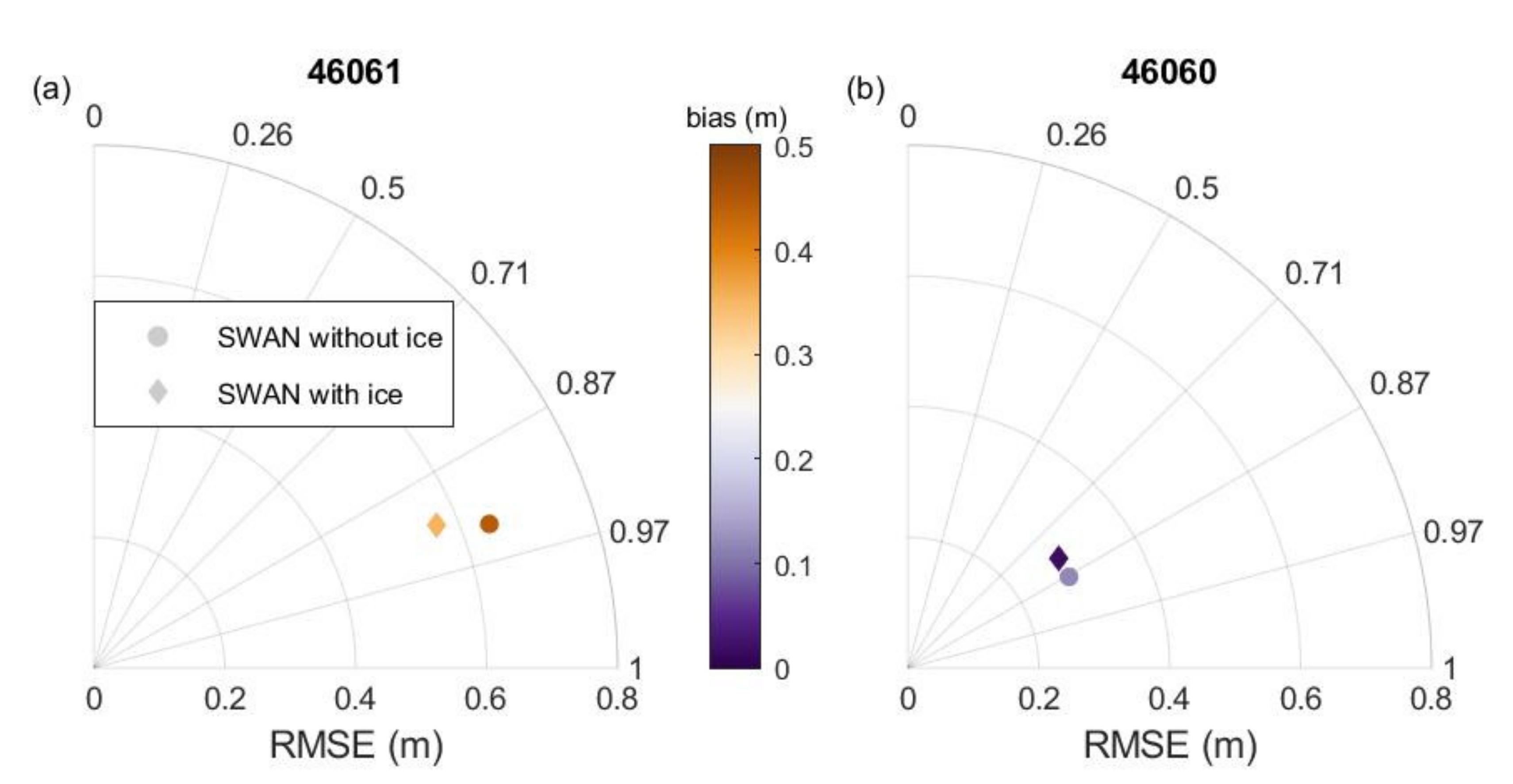
3.1. Model Validation

The modeled significant wave height, Hs, values agree dwell with the buoy values inside and outside PWS and the agreement improved when sea ice was accounted for in SWAN. Time series of the month of December for 2016–2019 show the agreement during times of large and small waves at both the buoy near the mouth of PWS, which encountered large waves, and the buoy inside PWS, where the waves were smaller (Figure 4). When no sea ice was present, the SWAN without ice output agreed with the SWAN with ice implementation and both models agreed well with the buoy data (14 December 2016, Figure 4a). During storms with sea ice, Hs was sometimes overestimated when SWAN was run without ice and Hs agreed better with the buoy data when SWAN was run with ice (8 December 2019, Figure 4g,h). Occasionally, the SWAN with ice implementation overly dampened wave heights due to the ice effect, and therefore, underestimated Hs (2 December 2017, Figure 4c).
The waves at buoy 46061 near the mouth of PWS were almost twice as large as the waves at buoy 46060 inside PWS, but at both buoys, the larger waves were overestimated when sea ice was not included in the model. This overestimation is shown in Figure 4g,h around December 8. Adding ice to the model corrected the overestimation and sometimes caused an underestimation of the wave heights (Figure 4c). A statistical comparison between buoy Hs values and model Hs values was computed with the commonly used error statistics: root mean square error (RMSE), bias, linear correlation coefficient (R), mean percentage error (PE), and scatter index (SI). These quantities are defined in Appendix A. Statistics of the model validation with and without ice are shown in Figure 5 and Table 2. The RMSE was improved at buoy 46061 from 0.64 m for the model without ice to 0.57 m for the model with ice (Figure 5a). At buoy 46060, the RMSE did not change when sea ice was added to the model (Figure 5b). The ice implementation lowered the bias at buoy 46061 from 0.44 m to 0.35 m and at buoy 46060 from 0.12 to 0.02 m (Figure 5). The linear correlation coefficient, R, decreased slightly when ice was added to the model at both locations. The percentage error decreased at both buoys with the ice implementation, and the scatter index decreased at 46061 but increased at 46060. The scatter index improved at buoy 46060 when sea ice was added to the model, with different coefficients describing the wave/ice interaction, as discussed in Section 3.2. Overall, the comparison statistics improved when ice was added to the model.
The effect of sea ice on the waves depends on the amount of sea ice present. Figure 6 shows how the modeled and measured Hs values changed with the sea ice concentration. The sea ice concentration was calculated at the location of buoy 46061 near the mouth of PWS. At that location, ice directly dampened waves measured by buoy 46061 and dampened waves that propagated into PWS and were measured by buoy 46060. Modeled versus measured Hs scatterplots that were separated by sea ice concentration (SIC) showed changes in the comparisons as the SIC increased from below 10% to above 40%. At buoy 46061, the linear regression was closest to the one-to-one line when the SIC was above 20% and below 30% (Figure 6c). At buoy 46061, the wave heights were overestimated by both the model without ice and with ice until the SIC was above 30%. When the SIC was above 30% the SWAN model with ice underestimated Hs at buoy 46061, whereas the SWAN model without ice still overestimated Hs (Figure 6d,e). At buoy 46060, the linear regression was above the one-to-one line for the model without ice until the SIC was greater than 40%. The model with ice lowered the linear regression close to the one-to-one line for all sea ice conditions when the SIC was less than 40%. When the SIC was greater than 40%, there were very few measurements at buoy 46060, and adding sea ice to the model did not change the comparison.

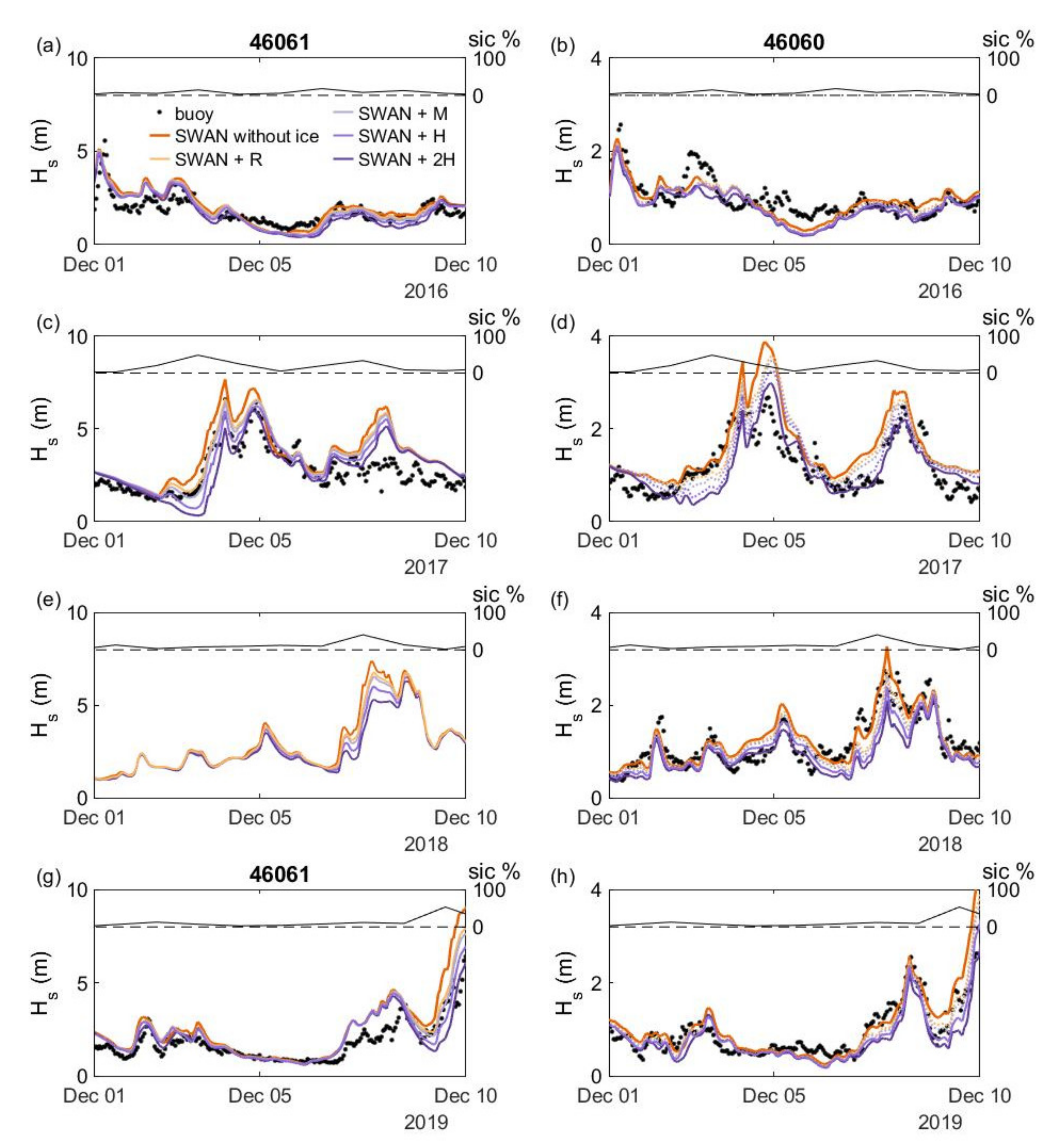
3.2. Parameterization of Sea Ice/Wave Interaction in SWAN

The sea ice/wave interaction parameterization in SWAN 41.31 uses sets of coefficients to model the dampening of waves by ice. The dependence of the wave heights on these coefficients was explored by running the model with the four sets of coefficients listed in Table 1 over the month of December in 2017. The coefficients were smallest for the pancake ice observed by Rogers et al., 2018, slightly larger for the 10–25 m floes observed by Meylan et al., 2014, and largest for the pancake and frazil ice observed by Hosekova et al., 2020. The Hosekova et al., 2020 coefficients were doubled to test the effect of larger coefficients. In the following tables and figures, the Rogers et al., 2018 coefficients are denoted by an R, the Meylan et al., 2014 coefficients are denoted by an M, the Hosekova et al., 2020 coefficients are denoted by an H, and two times the Hosekova et al., 2020 coefficients is denoted by 2H. Larger coefficients reduce wave heights more than smaller coefficients. The statistical comparison of a sensitivity test for December 2017 is shown in Table 3 and Figure 7. The RMSE, bias, R, PE, and SI values all decreased as the coefficients increased. A decrease in all parameters corresponded to an improvement in the model/buoy comparison except for the R value. The R value represented the correlation of the wave height signals in time. The sea ice dampening effect decreased the wave heights, and therefore, decreased the wave height changes in time, which decreased the R value of the comparison. The parameter that improved the most was the bias at buoy 46060. It decreased to zero when the 2H coefficients were used. The RMSE decreased the most at both buoys when using the 2H coefficients.
A longer sensitivity test was carried out by running the model with the four sets of coefficients for the month of December from 2016–2019. The results of this sensitivity test are shown in Figure 8 and Table 4. The improvements of the parameters at buoy 46061 are similar in pattern and magnitude to those from the single-month test. The parameters do not show as much change or improvement at buoy 46060 as they did in the single-month test. The bias and PE both are negative at buoy 46060 when the largest (2H) coefficients are used. This indicates that the model is dampening the waves too much.
The time series of the comparisons with buoy data are shown in Figure 9. When no ice was present, all five model implementations agreed (1 December 2017, Figure 9c). When ice was present, the wave heights decreased in size as the coefficients increased from R to M, H, and 2H coefficients (Figure 9). The agreement with buoy Hs values varied when the 2H coefficient implementation agreed best with the buoy and the other implementations overestimated the waves (7 December 2017, Figure 9d) when the 2H coefficient implementation underestimated the waves and the R coefficient implementation agreed well with the buoy (3 December 2017, Figure 9c).
Statistical comparisons of Hs predicted by the model implementations and measured by the buoy show the model implementation with the 2H ice coefficients predicted waves closest in size to those measured by buoy 46061 near the mouth of PWS. At buoy 46060, inside of PWS, the one-month sensitivity test showed the most improvement in the wave height comparison when the 2H coefficients were used, but the four-month sensitivity test found very little change in the RMSE with any of the coefficients and a negative bias when the 2H coefficients were used. The improvement in the comparison statistics when using the 2H statistics at buoy 46061 and at buoy 46060 in the one-month test demonstrated that the 2H coefficients best describe the wave/ice interaction at these two buoy locations. The 2H coefficients were used for the long model runs whose statistical comparisons to buoy data were reported in Table 2. Future research could improve the understanding of the coefficients by examining the ice type and thickness around PWS.

3.3. Effect of Sea Ice on the Wave Resource

Sea ice dissipates waves, and therefore, decreases the available power that could be extracted by a wave energy converter. Figure 10 shows examples of this decrease on 7 December 2017 when the AMSR2 satellite instrument measured ice around the edges and across the mouth of PWS (Figure 2a). The model that was run without sea ice showed wave heights above 1 m inside PWS (Figure 10a). When ice was added to the model simulation, the wave heights decreased significantly at the mouth of and inside PWS (Figure 10b). The decrease is shown as a difference in Figure 10c, where the difference is largest at the mouth of PWS. The decrease in Hs due to ice corresponds to a decrease in power.
The power from waves is defined in terms of the density of water, ρ , the acceleration due to gravity, g, the wavenumber, k, the water depth, h, and the significant wave height, Hs. It is calculated as the mean energy density, E, times the group wave velocity, cg, P = E c g . The mean energy density is given by linear wave theory as:
E = 1 16 ρ g H s 2
and the group velocity as:
c g = 1 2 c p 1 + 2 k h sinh ( 2 k h )
where the phase velocity is:
c p = g k tanh ( k h )
The wave power inside PWS was estimated to be larger when the model was run without ice than when it was run with ice (Figure 10d,e). The power difference is largest at the mouth of PWS and along the coasts of Montague and Hinchinbrook Islands (Figure 10f). At the mouth of PWS and along the coasts of Montague and Hinchinbrook Islands, the power was reduced from 100 kW/m to almost zero by the presence of sea ice. This decrease of wave power by up to 100 kW/m is a significant decrease that should be accounted for when assessing the wave power resource at that location. The wave power was also reduced landward of the mouth of PWS. This is associated with swells being dissipated by sea ice near the mouth because sea ice was only present near the shore and not in the middle of PWS during the study period. This will not only affect the magnitude of the wave power but also the frequency distribution at PWS.
The seasonal changes in available power were investigated by comparing the average monthly power computed from 2016–2020 (Figure 11). The maximum power difference due to sea ice occurred in December. Significant power differences occurred in January and February, minimal differences occurred in March, April, and May, and no power differences were detected in June, October, and November. The model was not run with the ice implementation for July, August, and September because no sea ice was present around PWS during those months.

4. Discussion and Conclusions

The sea ice/wave interaction addition to a high-resolution unstructured-grid SWAN model was used to investigate the dampening effects of sea ice on wave heights and wave power in PWS in Alaska. Wave heights and power decreased throughout PWS when sea ice was present, but the largest effects were seen at the mouth of the sound and along the coast of Montague Island. Sea ice was not observed to cover the sound entirely but the waves in the sound decreased when ice across the mouth impeded wave propagation from the ocean. This reduction in wave power was found to occur even on the northern coast of PWS.
Wave power was significantly reduced when sea ice was present. The strongest effect occurred at the mouth of PWS due to the large waves and high concentrations of sea ice. The power decrease changed seasonally with the sea ice and was maximum in December. Future wave resource assessments in Alaska should include the effects of sea ice, especially for the northern parts of Alaska, where significant amounts and time periods of ice cover occur.
The SWAN model was validated using buoy data from one buoy near the mouth and one inside the sound. The model–data comparison improved at both sites when sea ice was added to SWAN, but the improvement was greater at the buoy near the mouth due to strong ice concentrations at that location and larger waves than inside the sound. Four sets of sea ice dampening coefficients were evaluated in SWAN and were found to have varying impacts on the waves. The larger coefficients dampened the waves more than the smaller coefficients and occasionally decreased the wave heights so much that the wave heights were underestimated relative to the buoy measurements. The coefficients are defined by ice type such as pancake or large floes, but no satellite information is available yet that describes ice type. The satellite information input to this implementation of SWAN was a 3.125 km grid of daily ice concentration values, but no information about the type of ice, its thickness, or its change over the 24 h period was available.
The current sea ice implementation in SWAN only considers one set of coefficients for the entire model domain. Future research on the implementation of spatially varying ice type should be considered to improve the prediction of sea ice/wave interactions for locations where the sea ice type changes within the model domain. Large coefficients may be needed close to the coast where the ice is thick and old, but small coefficients may be needed in open water that features freshly formed pancake or frazil ice.

Author Contributions

Conceptualization, Z.Y., R.B., and G.G.-M.; methodology, R.B., G.G.-M., T.W., and F.T.R.; formal analysis, R.B.; writing—original draft preparation, R.B.; writing—review and editing, Z.Y., G.G.-M., R.B., F.T.R., and L.H.; visualization, R.B. and G.G.-M.; supervision, Z.Y.; project administration, Z.Y.; funding acquisition, Z.Y. All authors have read and agreed to the published version of the manuscript.

Funding

This study was funded by the U.S. Department of Energy, Office of Energy Efficiency and Renewable Energy, Water Power Technologies Office under contract DE-AC05-76RL01830 to Pacific Northwest National Laboratory (PNNL). All model simulations were performed using PNNL’s Institutional Computing facility. L.H. was funded by the US National Science Foundation (OPP 1818485). L.H. was also funded by the US National Science Foundation (OPP 1818485).

Data Availability Statement

Wave buoy data are available from NDBC at https://www.ndbc.noaa.gov/station_page.php?station=46061 (accessed on 30 April 2020) and https://www.ndbc.noaa.gov/station_page.php?station=46060 (accessed on 30 April 2020). Sea ice concentration data are available from ftp://ftp-projects.cen.uni-hamburg.de/seaice/AMSR2/3.125km/ and accessed on 30 April 2020. Model output is available by contacting [email protected].

Acknowledgments

The authors would like to thank Erick Rogers and Marcel Zijlema for help with the sea ice implementation in SWAN, Harry Stern for his help locating high-resolution sea ice concentration data, and Stefan Kern and Xiangshan Tian-Kunze for help obtaining the AMSR2 data.

Conflicts of Interest

The authors declare no conflict of interest.

Appendix A. Error Statistics

The error metrics used to evaluate model performance are the root mean square error (RMSE), mean percentage error (PE), scatter index (SI), bias, and the linear correlation coefficient (R):
R M S E = i = 1 N P i M i 2 N
P E = 100 N i = 1 N P i M i M i
S I = R M S E M ¯
b i a s = 1 N i = 1 N P i M i
R = i = 1 N P i P ¯ M i M ¯ i = 1 N P i P ¯ 2 i = 1 N M i M ¯ 2
where N is the number of measurements, Mi is the measured data, Pi is the predicted results, and overbars represent time averages.

References

  1. Chang, G.; Jones, C.A.; Roberts, J.D.; Neary, V.S. A comprehensive evaluation of factors affecting the levelized cost of wave energy conversion projects. Renew. Energy 2018, 127, 344–354. [Google Scholar] [CrossRef]
  2. Fairley, I.; Lewis, M.; Robertson, R.; Hemer, M.; Masters, I.; Horrillo-Caraballo, J.; Karunarathna, H.; Reeve, D.E. A classification system for global wave energy resources based on multivariate clustering. Appl. Energy 2020, 262, 114515. [Google Scholar] [CrossRef]
  3. Garcia-Medina, G.; Yang, Z.; Wu, W.; Wang, T. Wave resource characterization at regional and nearshore scales for the U.S. Alaska coast based on a 32-year high-resolution hindcast. Renew. Energy 2021, 170, 595–612. [Google Scholar] [CrossRef]
  4. Wadhams, P.; Squire, V.A.; Goodman, D.J.; Cowan, A.M.; Moore, S.C. The attenuation rates of ocean waves in the marginal ice zone. J. Geophys. Res. Ocean. 2018, 93, 6799–6818. [Google Scholar] [CrossRef]
  5. Doble, M.J.; Bidlot, J.-R. Wave buoy measurements at the Antarctic sea ice edge compared with an enhanced ECMWF WAM: Progress towards global waves-in-ice-modeling. Ocean. Model. 2013, 70, 166–173. [Google Scholar] [CrossRef]
  6. Meylan, M.H.; Bennetts, L.G.; Kohout, A.L. In situ measurements and analysis of ocean waves in the Antarctic marginal ice zone. Geophys. Res. Lett. 2014, 41, 5046–5051. [Google Scholar] [CrossRef]
  7. Doble, M.J.; De Carolis, G.; Meylan, M.H.; Bidlot, J.-R.; Wadhams, P. Relating wave attenuation to pancake ice thickness, using field measurements and model results. Geophys. Res. Lett. 2015, 42, 4473–4481. [Google Scholar] [CrossRef] [Green Version]
  8. Thomson, J.; Rogers, W.E. Swell and sea in the emerging Arctic ocean. Geophys. Res. Lett. 2014, 41, 3136–3140. [Google Scholar] [CrossRef]
  9. Gemmrich, J.; Rogers, W.E.; Thomson, T.; Lehner, S. Wave evolution in off-ice wind conditions. J. Geophys. Res. Ocean. 2018, 123, 5543–5556. [Google Scholar] [CrossRef]
  10. Thomson, J.; Ackley, S.; Girard-Ardhuin, F.; Ardhuin, F.; Babanin, A.; Boutin, G.; Brozena, J.; Cheng, S.; Collins, C.; Doble, M.; et al. Overview of the Arctic sea state and boundary layer physics program. J. Geophys. Res. Ocean. 2018, 23, 8674–8687. [Google Scholar] [CrossRef]
  11. Hosekova, L.; Malila, M.P.; Rogers, W.E.; Roach, L.A.; Eidam, E.; Rainville, L.; Kumar, N.; Thomson, J. Attenuation of ocean surface waves in pancake and pancake sea ice along the coast of the Chukchi Sea. J. Geophys. Res. 2020, 125, 1–15. [Google Scholar] [CrossRef]
  12. Zhang, N.; Li, S.; Wu, Y.; Wang, K.-H.; Zhang, Q.; You, Z.-J.; Wang, J. Effects of sea ice on wave energy flux distributions in the Bohai Sea. Renew. Energy 2020, 162, 2330–2343. [Google Scholar] [CrossRef]
  13. Zhang, Y.; Chen, C.; Beardsley, R.C.; Perrie, W.; Gao, G.; Zhang, Y.; Qi, J.; Lin, H. Applications of an unstructured grid surface wave model (FVCOM-SWAVE) to the Arctic Ocean: The interaction between ocean waves and sea ice. Ocean. Model. 2020, 145, 101532. [Google Scholar] [CrossRef]
  14. Yang, Z.; Wu, W.-C.; Wang, T.; Garcia-Medina, G.; Castrucci, L. High-Resolution Regional Wave Hindcast for the U.S. Alaska Coast. PNNL Rep. 2019. [Google Scholar] [CrossRef]
  15. Stopa, J.E.; Cheung, K.F.; Chen, Y.-L. Assessment of wave energy resources in Hawaii. Renew. Energy 2011, 36, 554–567. [Google Scholar] [CrossRef]
  16. Li, N.; Cheung, K.F.; Stopa, J.E.; Hsiao, F.; Chen, Y.-L.; Vega, L.; Cross, P. Thirty-four years of Hawaii wave hindcast from downscaling of climate forecast system reanalysis. Ocean. Model. 2016, 100, 78–95. [Google Scholar] [CrossRef] [Green Version]
  17. Wu, W.-C.; Yang, Z.; Wang, T. Wave resource characterization using an unstructured grid modeling approach. Energies 2018, 11, 605. [Google Scholar]
  18. Wu, W.-C.; Wang, T.; Yang, Z.; Garcia-Medina, G. Development and validation of a high-resolution regional wave hindcast model for US West Coast wave resource characterization. Renew. Energy 2020, 152, 736–753. [Google Scholar] [CrossRef]
  19. Booij, N.; Ris, R.C.; Holthuijsen, L.H. A third-generation wave model for coastal regions 2. Model description and validation. J. Geophys. Res. 1999, 104, 7646–7666. [Google Scholar] [CrossRef] [Green Version]
  20. Ris, R.C.; Holthuijsen, L.H.; Booij, N. A third-generation wave model for coastal regions 2. Verification. J. Geophys. Res. 1999, 104, 7667–7681. [Google Scholar] [CrossRef]
  21. Rogers, W.E. Implementation of Sea Ice in the Wave Model SWAN; Technical Report; Naval Research Lab.: Washington, DC, USA, 2019. [Google Scholar]
  22. Rogers, W.E.; Thomson, J.; Shen, H.H.; Doble, M.J.; Wadhams, P.; Cheng, S. Dissipation of wind waves by pancake and frazil ice in the autumn Beaufort Sea. J. Geophys. Res. 2016, 121, 7991–8007. [Google Scholar] [CrossRef] [Green Version]
  23. Canals Silander, M.F.; Garcio Moreno, C.G. On the spatial distribution of the wave energy resource in Puerto Rico and the United States Virgin Islands. Renew. Energy 2019, 136, 442–451. [Google Scholar] [CrossRef]
  24. Li, N.; Garcia-Medina, G.; Cheung, K.F.; Yang, Z. Wave energy resources assessment for the multi-modal sea state of Hawaii. Renew. Energy 2021, 174, 1036–1055. [Google Scholar] [CrossRef]
  25. Ahn, S.; Neary, V.S.; Allahdadi, M.N.; He, R. Nearshore Wave Energy Resource Characterization along the East Coast of the United States. Renew. Energy 2021, 172, 1212–1224. [Google Scholar] [CrossRef]
  26. Yang, Z.; Garcia-Medina, G.; Wu, W.-C.; Wang, T. Characteristics and variability of the nearshore wave resource on the US West Coast. Energy 2020, 203, 117818. [Google Scholar] [CrossRef]
  27. Zijlema, M. Computation of wind-wave spectra in coastal waters with SWAN on unstructured grids. Coast. Eng. 2010, 57, 267–277. [Google Scholar] [CrossRef]
  28. Lim, E.; Eakins, B.W.; Wigley, R. Coastal Relief Model of Southern Alaska: Procedures Data Sources and Analysis; NOAA Technical Memorandum NESDIS NGDC-43; National Geophysical Data Center: Boulder, CO, USA, 2011. [Google Scholar]
  29. Zimmermann, M.; Prescott, M.M. Smooth Sheet Bathymetry of the Aleutian Islands; NOAA Technical Memorandum NMFS-AFSC-250; National Geophysical Data Center: Boulder, CO, USA, 2013. [Google Scholar]
  30. Zimmermann, M.; Prescott, M.M. Smooth Sheet Bathymetry of Cook Inlet Alaska; NOAA Technical Memorandum NMFS-AFSC-275; National Geophysical Data Center: Boulder, CO, USA, 2014. [Google Scholar]
  31. Zimmermann, M.; Prescott, M.M. Smooth Sheet Bathymetry of the Central Gulf of Alaska; NOAA Technical Memorandum NMFS-AFSC-287; National Geophysical Data Center: Boulder, CO, USA, 2015. [Google Scholar]
  32. Hasselmann, K.; Barnett, T.P.; Bouws, E.; Carlson, H.; Cartwright, D.E.; Enke, K.; Ewing, J.A.; Gienapp, H.; Hasselmann, D.E.; Krusemann, P.; et al. Measurements of Wind-Wave Growth and Swell Decay during the Joint North Sea Wave Project (JONSWAP); Deutches Hydrographisches Institut: Hamburg, Germany, 1973; pp. 1–95. [Google Scholar]
  33. Battjes, J.A.; Janssen, J.P.F.M. Energy loss and set-up due to breaking of random waves. In Proceedings of the 16th International Conference on Coastal Engineering, ASCE, Hamburg, Germany, 27 August–3 September 1978; pp. 569–587. [Google Scholar]
  34. Eldeberky, Y.; Battjes, J.A. Spectral modeling of wave breaking: Application to Boussinesq equations. J. Geophys. Res. 1996, 101, 1253–1264. [Google Scholar] [CrossRef]
  35. Saha, S.; Moorthi, S.; Wu, X.; Wang, J.; Nadiga, S.; Tripp, P.; Behringer, D.; Hou, Y.-T.; Chuang, H.-Y.; Iredell, M.; et al. The NCEP climate forecast system Version 2. J. Clim. 2014, 27, 2185–2208. [Google Scholar] [CrossRef]
  36. Chawla, A.; Spindler, D.M.; Tolman, H.L. Validation of a thirty year wave hindcast using the Climate Forecast System Reanalysis winds. Ocean. Model. 2013, 70, 189–206. [Google Scholar] [CrossRef]
  37. Kaleschke, L.; Lupkes, C.; Vihma, T.; Haarpainter, J.; Bochert, A.; Hartmann, J.; Heygster, G. SSM/I sea ice remote sensing for mesoscale ocean-atmosphere interaction analysis. Can. J. Remote Sens. 2001, 27, 526–537. [Google Scholar] [CrossRef]
  38. Beitsch, A.; Kaleschke, L.; Kern, S. Investigating high-resolution AMSR2 sea ice concentrations during the February 2013 fracture event in the Beaufort Sea. Remote Sens. 2014, 6, 3841–3856. [Google Scholar] [CrossRef] [Green Version]
Figure 1. Sea ice concentration at four times of year in Alaska as measured by the Advanced Microwave Scanning Radiometer 2 (AMSR2) instrument. (a) Spring: 15 March 2017; (b) Summer: 15 June 2017; (c) Fall: 15 September 2017, with a red box outlining the study area of Prince William Sound; (d) Winter: 15 December 2017.
Energies 14 03482 g001
Figure 2. (a) Example of ice concentrations around PWS as measured with the AMSR2 instrument on 7 December 2017. Both sea ice and land ice are shown. Red circles indicate the locations of wave buoy 46060 inside PWS and 46061 near the mouth. (b) Comparison of the modeled significant wave height, Hs, and the measured Hs at buoy 46061 during 2017 (data from [14]).
Energies 14 03482 g002
Figure 3. (a) Bathymetry grid input to SWAN with the locations of Montague and Hinchinbrook Islands marked at the mouth of PWS. (b) Resolution of the unstructured grid used in SWAN.
Energies 14 03482 g003
Figure 4. Significant wave height, Hs, as measured by wave buoys and modeled by SWAN with and without ice in December of 2016–2019 (left axis). Sea ice concentration calculated from AMSR2 data at the location of buoy 46061 with the zero line marked as dashed (right axis). (a,c,e,g) Comparisons at wave buoy 46061 near the mouth of PWS. (b,d,f,h) Comparisons at wave buoy 46060 inside of PWS where the waves are smaller. Data were missing from buoy 46061 for part of December 2018.
Energies 14 03482 g004
Figure 5. Root mean square error, correlation coefficient, and bias of comparisons between the SWAN model and the buoys for data from 2016–2020. The RMSE is the distance from the origin, the correlation coefficient is shown as the angle from the y-axis, and the bias is the shown as the color of the marker. (a) The comparison at buoy 46061 near the mouth of PWS; (b) the comparison at buoy 46060 inside PWS.
Energies 14 03482 g005
Figure 6. Modeled versus measured significant wave heights, Hs, at buoy 46061 (ae) and 46060 (fj) for increasing amounts of sea ice concentration (SIC). Sea ice concentrations were calculated from AMSR2 data at the mouth of PWS. The gray line is the one-to-one line, the orange line is the linear regression of the SWAN only model to the buoy data, and the black line is the linear regression of the SWAN model with ice to the buoy data.
Energies 14 03482 g006
Figure 7. Root mean square error, correlation coefficient, and bias of comparisons between the SWAN model and the buoys for the month of December 2017. The RMSE is the distance from the origin, the correlation coefficient is shown as the angle from the y-axis, and the bias is shown as the color of the marker. (a) The comparison at buoy 46061 near the mouth of PWS; (b) the comparison at buoy 46060 inside PWS.
Energies 14 03482 g007
Figure 8. Root mean square error, correlation coefficient, and bias of comparisons between the SWAN model and the buoys for the month of December from 2016–2019. The RMSE is the distance from the origin, the correlation coefficient is shown as the angle from the y-axis, and the bias is the shown as the color of the marker. (a) The comparison at buoy 46061 near the mouth of PWS; (b) the comparison at buoy 46060 inside PWS.
Energies 14 03482 g008
Figure 9. Significant wave height, Hs, near the mouth of and inside PWS as measured by wave buoys and modeled by SWAN without ice and with wave/ice interactions modeled with four different sets of coefficients for the first 10 days of December of 2016–2019. Sea ice concentration is shown on the right axis as a black line and 0% is shown as a dashed black line. (a,c,e,g) Comparisons at wave buoy 46061 at the mouth of PWS. (b,d,f,h) Comparisons at wave buoy 46060 inside of PWS where the waves are smaller. Buoy data were missing for the first 10 days of December 2018 at buoy 46061.
Energies 14 03482 g009
Figure 10. Comparisons of significant wave height, Hs, and power in model output of 7 December 2017, when significant sea ice was present, as shown in Figure 3b. (a) Hs as calculated by SWAN run without ice; (b) Hs as calculated by SWAN run with ice; (c) Hs difference between the SWAN runs with and without ice; (d) power from SWAN run without ice; (e) power from SWAN run with ice; and (f) power difference between SWAN runs with and without ice.
Energies 14 03482 g010
Figure 11. Prince William Sound: average power difference between the SWAN model without ice and the SWAN model with ice computed from 2016–2020. (a) January, (b) February, (c) March, (d) April, (e) May, (f) June, (g) October, (h) November, (i) December.
Energies 14 03482 g011
Table 1. Coefficients used in SWAN to model sea ice/wave interactions. Hereafter, the sets of coefficients will be referred to by the bold initials.
CoefficientRogers et al., 2018Meylan et al., 2014Hosekova et al., 20202H 1
C2 (s2 m−1)0.284 × 10−31.06 × 10−33.8 × 10−37.6 × 10−3
C4 (s4 m−1)1.53 × 10−22.3 × 10−21.8 × 10−23.6 × 10−2
1 H2 = two times the Hosekova et al., 2020 coefficients.
Table 2. SWAN model performance with and without ice at buoys 46061 and 46060. Statistics were calculated from 28,191 comparisons over the years of 2016–2020, excluding July, August, and September.
ModelRMSE (m)Bias (m)RPE (%)SI
46061460604606146060460614606046061460604606146060
SWAN no ice0.640.280.440.120.940.8731.5222.830.330.33
SWAN + ice0.570.280.350.020.920.8126.9410.560.310.37
Table 3. SWAN model performance with no ice and four sets of ice coefficients during December 2017. The coefficients are listed from the smallest (0 for no ice) to the largest (2H).
ModelRMSE (m)Bias (m) R PE (%) SI
46061460604606146060460614606046061460604606146060
SWAN no ice1.000.470.730.310.920.9030.7331.460.440.44
SWAN + R0.900.450.650.250.930.8727.8326.770.390.42
SWAN + M0.870.420.600.210.920.8622.6422.640.380.39
SWAN + H0.820.390.500.120.900.8421.8614.140.360.37
SWAN + 2H0.810.370.350.000.860.8215.962.500.350.34
Table 4. SWAN model performance with no ice and four sets of ice coefficients during December of 2016–2019.
ModelRMSE (m) Bias (m) R PE (%) SI
46061460604606146060460614606046061460604606146060
SWAN no ice0.820.360.560.130.930.8628.8314.320.390.35
SWAN + R0.730.330.480.070.930.8422.267.930.340.33
SWAN + M0.690.330.430.030.920.8320.354.480.330.32
SWAN + H0.640.330.35−0.040.910.9116.61−1.980.310.32
SWAN + 2H0.620.350.23−0.130.890.8911.42−10.540.290.34
Publisher’s Note: MDPI stays neutral with regard to jurisdictional claims in published maps and institutional affiliations.

