
Evaluation of ICEYE Microsatellites Sensor for Surface Motion Detection—Jakobshavn Glacier Case Study


Faculty of Mining Surveying and Environmental Engineering, AGH University of Science and Technology, 30-059 Cracow, Poland
*
Author to whom correspondence should be addressed.
Energies 2021, 14(12), 3424; https://doi.org/10.3390/en14123424
Submission received: 18 May 2021
/
Revised: 2 June 2021
/
Accepted: 8 June 2021
/
Published: 10 June 2021
(This article belongs to the Special Issue Climate Change, Ecosystems and Environmental Geology: Threats, Challenges and Solutions in the Arctic)
Abstract
:The marine-terminating glaciers are one of the biggest contributors to global sea-level rise. Research on this aspect of the effects of global climate change is developing nowadays in several directions. One of them is monitoring of glaciers movements, especially with satellite data. In addition to well-known analyzes based on radar data from available satellites, the possibility of studying glacier displacements from new sensors, the so-called microsatellites need to be studied. The main purpose of research was evaluation of the possibility of applying new high-resolution ICEYE radar data to observe glacier motion. Stripmap High mode were used to obtain velocities for the Jakobshavn glacier with an Offset-Tracking method. Obtained results were compared with displacements obtained from the Sentinel-1 data. The comparative analysis was performed on displacements in range and azimuth directions and for maximum velocity values. Moreover, correlation plots showed that in different parts of glaciers, a comparison of obtained velocities delivers different correlation coefficients (R2) in a range from 0.52 to 0.97. The analysis showed that the scale of movements is similar from both sensors. However, Sentinel-1 data present underestimation of velocities comparing to ICEYE data. The biggest deviations between results were observed around the maximum velocities, near the Kangia Ice Fjord Bay. In the analysis the amplitude information was used as well. This research presents that data from the ICEYE microsatellites can be successfully used for monitoring glacial areas and it allows for more precise observations of displacement velocity field.
1. Introduction
Observing the ice-sheet all over the world is recently a topic of increasing importance, especially in the face of a constantly warming climate. Faster decreasing of ice masses in polar regions leads to sea-level rise [1]. Moreover, rapid detachment of the large parts of mountain glaciers causes a direct threat to human safety. Melting of ice cover and glaciers in Greenland is one of the main contributors to global sea-level rise in the world. Due to that fact, it is essential to monitor and get to know better this phenomenon. What is more, probably in perspective of few decades, the melting process will intensify [2]. Observing such movements and analysis of their dynamics changes over the years, provide us information that is necessary for a better understanding of the phenomenon that occurs in these areas [3]. Such knowledge allows better estimation of the pace of glaciers melting, the results of this process, and determining the causes of an increase in the speed of glacier motions [4].
Monitoring of glacier regions has been the subject of research for scientists from different disciplines for many years. At the beginning in-situ measurements were the only way to monitor glacial areas. However more secure methods of the monitoring were developed such as a photogrammetric survey [5]. The development of remote sensing techniques made it possible to observe these areas in a more accurate way also from a space. Optical imagery has found its application in monitoring changes in the position of the glacier fronts [6], as well as in determining the speed of their movement. For these purposes, the feature tracking method was developed [7,8]. It allows for determining the speed of chosen area by analyzing the changes of the positions of the characteristic objects on a series of images [9]. Further technological development and the appearance of high-resolution multispectral images increased the accuracy of observations [10]. An important aspect in studying glaciers is determining the thickness of the glacial cover, as well as its changes over time. For this reason, to determine the vertical changes in glacial areas are used such methods like altimetry [11] and radar interferometry, which allows the creation of high-quality digital terrain models [12,13,14,15,16,17].
However, the advent of satellite radar imagery made it possible to start monitoring glaciers with greater precision and regardless of the current weather conditions. The differential interferometry technique (DInSAR), which is applied in many world’s regions, allows determination of displacement with high accuracy, but it has some limitations. Changes that appear in areas of snow cover or mountain glaciers are characterized by the relatively high speed of daily changes, which causes a significant decrease in signal coherence in these areas [18]. For this reason, DInSAR is not always the appropriate method to obtain reliable results, despite satisfactory results in some areas [19,20]. The alternative method for determining displacements in the glacial regions is an Offset-Tracking (OT) technique, that uses information about the intensity of reflected signal [21,22,23,24]. This technique has found wide application not only in glacial regions but also in mapping other rapidly changing areas like earthquakes [25], volcanoes [26] or even mining areas [27]. This technology is usually used to determine displacements in range and azimuth direction. Other researchers started to determine vertical displacements with the use of data from different orbits or combining offset tracking method with differential interferometry [28,29]. The combination of these methods makes it possible to determine a complete velocity vector in the area where the intensity of movements is very diverse [30]. These studies are particularly important because they allow better estimation of changes in the balance of glacial masses [31]. Furthermore, it is possible to assess changes in the thickness of ice cover and estimate the contribution of individual glaciers to sea-level rise, especially considering independent altitude or meteorological data. Accurate analysis of velocities obtained from offset tracking technique improved possibilities of analyzing accelerations and deformations in glacial areas, which can lead to interruption of their surface [32]. Due to that fact, detecting spots where fissures can show up and monitoring the intensity of the calving process is possible [33]. The offset tracking method has many applications in both mountain glaciers [34,35,36] and polar regions [37,38,39]. It allows for almost real-time mapping of entire regions, such as Greenland [40] or Antarctica [41]. Moreover, usage of radar data improved investigation of such problems like ice classifications [42] or assessment of the grounding line position [43,44,45]. Thanks to that it is possible to show the impact of e.g., increase of average air temperature on glacier’s terminus retreat [46]. Other researchers focused on a problem connected with superglacial lakes drainage and its influence on changes in glaciers speeds [47,48], or usage of SAR data for better understanding the surge process [49].
Despite there are plenty of researches using the offset tracking method, its precision is usually determined as 1/10–1/30 of the pixel size of used SAR images [50]. An increase in data resolution can improve the accuracy of detected movements and analysis of short and dynamic changes such as calving events. What is more, in the case of marine-terminating glaciers, smaller terrain pixel allows more precise determination of terminus position. Because of it, areas of floating ice where the waving of water causes vertical movements can be excluded from the analysis. This research aim is to check the possibilities of using high-resolution radar images from ICEYE microsatellites to observe glaciers. Comparative analyses were performed with the use of Sentinel-1 data. Publicly available data from the Sentinel-1 satellites provide data with a resolution nearly four times lower than that of the ICEYE microsatellites. ICEYE mission started in January 2018 and delivers images with a resolution up to 0.25 m. So far new data from microsatellites has not been analyzed in terms of the possibility of using their potential for applications in glacial regions. This article presents a comparison of the results obtained from the Sentinel-1 and ICEYE mission. It shows the advantages and disadvantages of both data sources in the analysis of glaciers velocities on selected example.
2. Materials and Methods
2.1. Study Area
The research was carried out for the Jakobshavn glacier located in the western part of Greenland (Figure 1). So far it was one of the fastest moving glaciers in the world. Its record speed reached 46 m/day in 2012–2014 [51]. The glacier covers an area of 110,000 km2, its length is about 65 km, and the estimated thickness reaches 2 km. Because of its record speeds that vary over the years, the Jakobshavn glacier became the object of diverse research. Already in the 90s of the twentieth century, using the possibilities of satellite imagery, the changes of this glacier over 30 years were observed [52]. This research showed that the retreat of glacier terminus is slowing down. There also have been significant increases in calving rate during periods of higher temperatures. Moreover, the influence of ocean temperature changes and tides on velocities and glacier thickness was investigated [53,54]. The influence of ice melange on the position of the glacier front and its stability was also analyzed [55].
2.2. Satellite Mission Overview
In this research, new high-resolution radar images from ICEYE satellites were used. They are included in the microscale due to the small size of the sensors. Their weight reaches approx. 85 kg. Currently, the constellation consists of 10 satellites X1–X10 [56]. These satellites work in an X-band at a frequency of 9.65 GHz with left and right look directions. ICEYE offers products acquired in two modes: Spotlight (High) and Stripmap (High). The highest accuracy can be obtained for images collected in Spotlight High mode where pixel size reaches the value of 0.25 m. Scenes cover an area of 25 km2 (5 km × 5 km). The ICEYE sensors are imaging only in vertical polarization (VV) and deliver images with only amplitude information (Ground Range Detected—GRD) or amplitude and phase information (Single Look Complex—SLC). Due to the extensive research area, Stripmap High products were used. This mode is imaging in strips of 30 km × 50 km (approx. 1500 km2) with a resolution of 0.5 m × 3 m. Due to the kind of applied method, GRD products with a square field pixel were used, ultimately achieving a spatial resolution of 2.5 m × 2.5 m.
The results for the Jakobshavn glacier calculated based on ICEYE products were compared with the result from the Sentinel-1 satellites. The Sentinel-1 mission consists of 2 satellites imaging in C-band at a 5.4 GHz frequency. The mass of 1 satellite is about 945 kg (10 times more than the ICEYE satellite). Orbiting the Earth in tandem (Sentinel-1A and Sentinel-1B), they can deliver images every 6 days. In research were used images acquired in the Interferometric Wide (IW) mode. Data are collected in passes with the width of 250 km and with the resolution reaching in range and azimuth directions: from 2.7 m × 22 m to 3.5 m × 22 m. SAR images are acquired in two kinds of polarization: HH and HV. For purposes of this research horizontal polarization was used. Data from the Sentinel-1 satellites are available in few formats but for velocities calculation, products from level-1 (GRD) were used. These images have pixel size 10 m × 10 m. In the case of ICEYE satellites, the pixel size of images was 4 times smaller than for Sentinel-1 products.
2.3. Data and Method
For purposes of this research images for the Jakobshavn glacier from 5 and 9 January 2021 for the ICEYE mission and from 3 and 9 January 2021 for the Sentinel-1 mission have been used (Table 1).
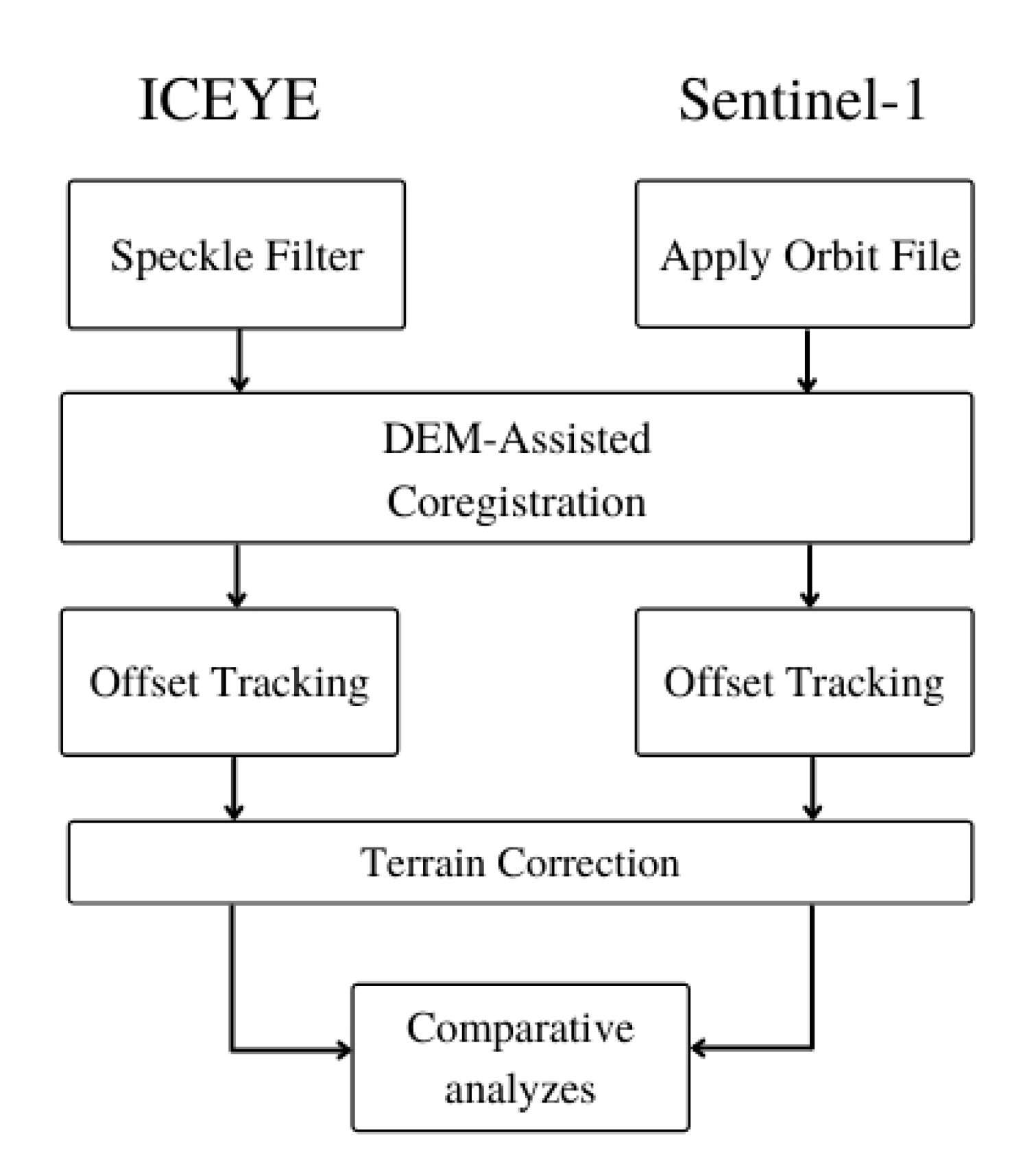
The displacements of the Jakobshavn glacier were calculated with an Offset-Tracking method. The preparation of data was different for both sensor types (Figure 2). In the case of the Sentinel-1 data, in the first step precise orbits were attached to each SAR image. The ICEYE products contain this information and due to that, in first stage speckle filtering was applied. This step is required due to the fact, that SAR images have inherent like “salt and pepper” texturing called speckles. It degrade the quality of the image and make interpretation of features more difficult. Spatial filtering reduce significant speckle noise. In analysis the Lee-Sigma filter was used as the best compared to other filters [57]. An alternative option is using multilooking processing to speckle noise reduction [58], but in this case, the image resolution is changed as a result of aggregation of pixel in groups. The aim of this research was to check the effectiveness of ICEYE products also resulting from high resolution images, therefore this solution has not been tested.
Further calculation steps were similar for both sensors. For image coregistration, Copernicus Digital Elevation Model with a 30 m resolution was used. Then, on image pairs, groups of pixels with corresponding intensities of reflection were searched. In this process, the image is searched with a registration window. Its size depends on the maximum predicted velocity of the analyzed area. Corresponding points called Ground Control Points (GCP) are searched for in a given area. Afterward, the distance between these points is calculated and then it is converted into the velocity of the object. For both sensors, the calculation parameters were selected (Table 2) so that the results were of the same resolution in a 100 m by 100 m grid. In the last stage, the obtained results were geo-referenced to perform comparative analyzes in one coherent reference system. Characteristic glacier areas were selected to create correlation plots from results obtained from ICEYE and Sentinel-1 data. Due to different time interval of analysis from ICEYE and Sentinel-1, the shift in range and azimuth direction was converted into the velocity values. This allowed to compare the results from both sensors despite differences in acquisitions dates. The correlation coefficients were calculated for movements in range and azimuth directions, and maximum velocities. The changes along the glacier profile are also presented. To assess changes in the bay area, the amplitude images showing terminus position and snow-ice cover were used.
3. Results
The obtained results allowed us to determine the displacements in the Jakobshavn glacier area, illustrating the pace of changes at the beginning of January 2021. The calculation period for the Sentinel-1 mission was 6 days and for ICEYE data—4 days. For this reason, analyses were performed on velocities in range and azimuth directions and maximum velocities in m/day (Figure 3).
Data from the ICEYE microsatellite show positive displacements in the range direction in snow cover surrounding the Jakobshavn Glacier. For Sentinel-1 data values in this region have opposite signs. In the area of main glacier flow, the movement pattern is similar on both results with negative vales suggesting displacement in Kangia Ice Fjord Bay direction (Figure 3). In the case of movements in the azimuth direction, both sensors show a clear separation of the positive value from the negative value. The displacement distribution in the bay area is also different.
The distribution of maximum velocities is comparable for both sensors, especially in parts located deeper in the land. The differences in the results are increasing with approaching the terminus and the bay. Both velocities obtained from Sentinel-1 and ICEYE data show an increase in speed in the bay direction. Despite the similar spatial distribution of observed movements, there are differences in the bay area. The maximum velocity from high-resolution ICEYE data reaches 41 m/day. For Sentinel-1 data, maximum velocity reaches the values of 36 m/day in a similar location.
The calculated velocities for both sensors were compared on a correlation plots in 4 different testing areas (Figure 4). For analysis purposes, the regions of the diverse dynamics were selected. The first testing area is in the inland part of the glacial tongue with relatively slow speeds (area 1). The next field is in the area of bigger displacements values (area 2). The next regions are part of the glacier with higher intensity of movements (area 3) and surrounding of the terminus position (area 4). The sizes of the testing areas were selected to cover only the area of the glacial tongue, without its surroundings. Due to the low velocities in the tail of the glacier and its widening in this region, the 1st area is the largest. Fields 2 and 3 have a similar size. Area 4 has the smallest size so that the speeds compared with each other are located only in the glacier front, where the movements reach their maximum values. For selected areas, correlation plots were defined for the range and azimuth movements as well as for the maximum values. In addition, along the entire glacier, a profile was selected to show speed changes obtained from Sentinel-1 and ICEYE data in the whole area.
In selected areas, point grids were generated and information about velocities from both sensors was extracted. The values are presented in correlation plots for each of the analyzed regions (Figure 5). The obtained correlation coefficients (R2) were in the range from 0.52 to 0.97. For all testing areas, the highest values were obtained for displacements in the azimuth direction. Excluding the area of the glacier terminus, R2 for this component was in the range 0.96–0.97. In the case of displacements in range direction, coefficients reached lower values in a wide range from 0.52 to 0.93. Area 3 is the most consistent in the results obtained from both sensors. The correlation coefficient for the maximum velocities was 0.93. Also in this area, data from both ICEYE and Sentinel-1 provided results with almost the same values, hence the fitted trend line is very close to the y = x function. The biggest differences in calculated velocities were obtained in area 4—the area of the terminus position. The correlation coefficient in this area is 0.71 but there are significant deviations between the results from both sensors are visible. The plot show the underestimation of the speed values in Sentinel-1 data comparing to ICEYE results. The results in areas 1 and 2 are quite similar. These regions reflect slower parts of a glacier. In the case of the azimuth component, the R2 reaches a value of 0.96. A significantly lower correlation is visible on graphs for the range component. The correlation coefficient is in the range from 0.52 to 0.56.
In the last stage of the analysis, a profile was drawn along the entire glacier through its central part. Along the profile, information was collected on the velocities measured by both sensors depending on the distance from the glacier front (Figure 6). For both sensors, the maximum velocities are achieved just beyond the front of the glacier. The process of glacier movement slows down with the distance from the terminus. Both profiles agree to the value and nature of the phenomenon. In some parts of the Jakobshavn glacier, an underestimation of velocity calculated from Sentinel-1 data is visible. The most dynamic changes are in the area where a glacier flows to the bay. The biggest deviations between results from both sensors are observed in this region. The differences are at the level of a few m/day.
4. Discussion
The use of higher resolution data from the ICEYE microsatellites showed higher velocities in the glacier front region with a difference of +5 m/day (14%) compared to the results from the Sentinel-1 data. Due to difference in pixel size of the Sentinel-1 and ICEYE data, it can be concluded that the obtained differences in observations are significant and show higher values of movements observed with the use of high-resolution ICEYE data. This may result from the OT method itself, which, by aggregating a group of pixels, assigns them averaged values of movements. A higher resolution of the ICEYE data allows the detection of changes in smaller areas compared to the Sentinel-1 satellite. This is also visible in greater diversification of the pattern of movements visible in the displacement distributions. The results from the Sentinel-1 satellite data are smoother than those from the ICEYE data (Figure 4).
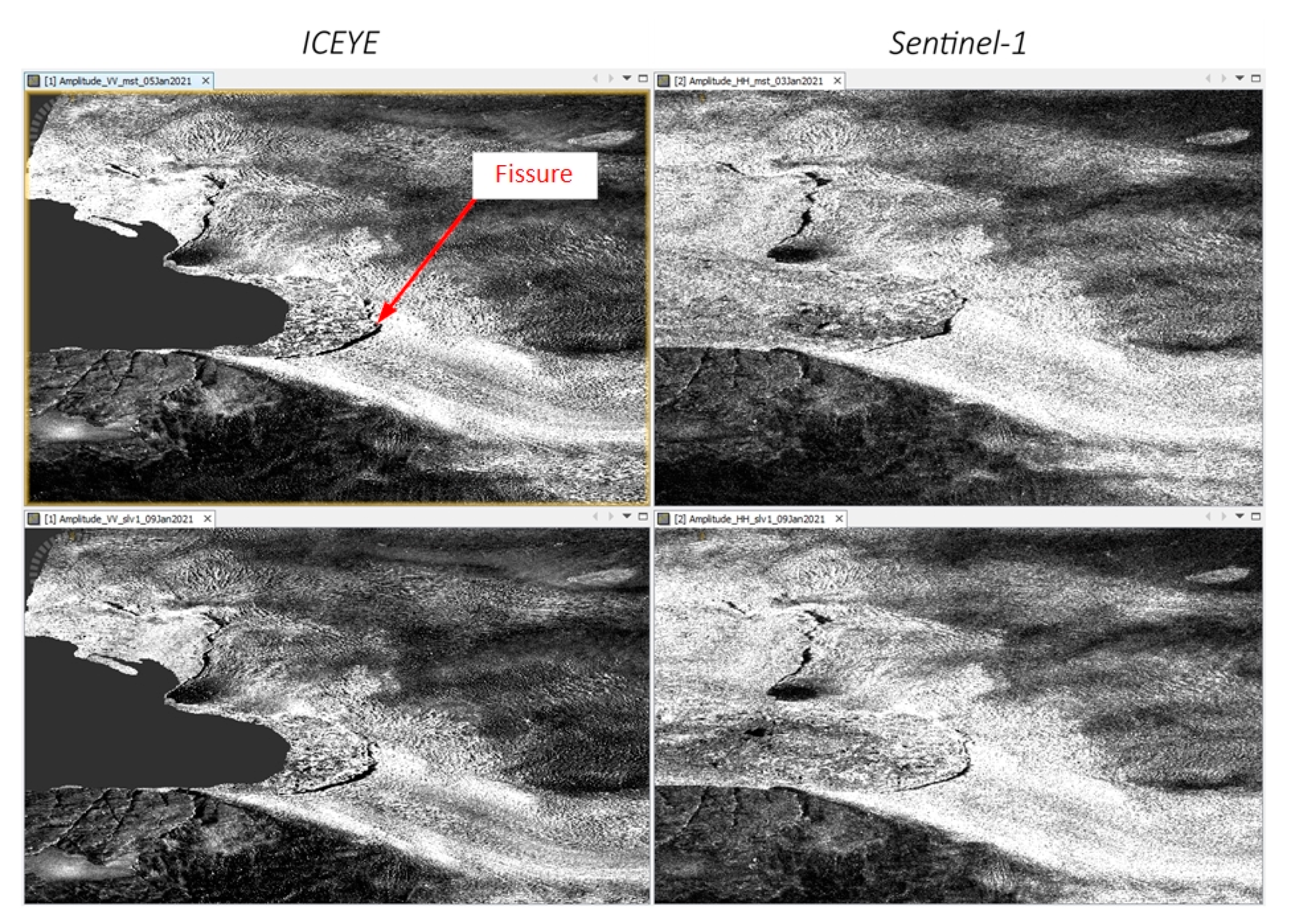
The analyzes performed on the profile data show that the difference in the observed velocities does not depend on the scale of the phenomenon, except the Kangia Ice Fjord Bay area. The differences in this area may occur due to floating snow-ice cover in the bay. This cover is clearly visible in the photos presenting the amplitude values (Figure 7). In the case of the Sentinel-1 products, there is no visible cut-off of the glacial tongue from the snow-ice cover floating in the waters of the bay. On the product from the ICEYE microsatellite, the terminus can be clearly distinguished from the waters in the bay with a small part of snow-ice masses. These parts of floating materials are registered in the calculation process as smaller movements in the front of the glacier. In addition, the images from 9 January show large variations in the Kangia Bay area despite the data collection on the same day. This is due to the different polarization of both sensors. In case of Sentinel-1 it is horizontal polarization (HH) in relation to ICEYE product with vertical polarization (VV) of radar signal.
A higher resolution of the ICEYE images allows a more precise determination of the glacier border or the location of the fissures. It is especially important in terms of the displacement analysis, to distinguish the part of the glacier which is located on stable land from floating sea-ice. In both images, this border in the central part of the glacier is visible because of the big width of the fissure between both parts (Figure 7). The SAR images from ICEYE make it possible to determine this border in a more accurate way in the side parts of the glacier.
5. Conclusions
Comparative research on the movement of the Jakobshavn glacier carried out based on the offset tracking method and images from the Sentinel-1 and ICEYE satellites allowed for an unequivocal determination of the glacier’s speed throughout the entire observation range. As research shows, a higher resolution of ICEYE products compared to S-1 allows more precise identification of glacier details, especially in the terminus area. Imaging of the floating ice on S-1 is impossible. Thanks to the higher resolution, detection of velocities in different parts of the glaciers based on ICEYE data gives slightly higher values comparing to S-1. This can be an effect of an averaging pixels with larger areas in S-1 data. It can be clearly seen in the front of the glacier. These differences reach values approx. 14% of Sentinel-1 velocity. The researches carried out so far derived information about movements to 46 m/day [51]. In selected for this research period, the maximum velocity was about 36 m/d for S-1 data and 41 m/d for ICEYE data. In the presented research, the scale of these speeds was confirmed by analyzing the images of the ICEYE satellite, but the results show that the Jakobshavn glacier is slightly slowing down. Such promising results allow the planning of further research on the possibilities of glacier displacement detection based on ICEYE microsatellites, especially about the accuracy of determining the displacement and velocity vectors. The use of new sensors from microsatellites opens up new possibilities in the prediction and future trends in the problem of glacier calving. Thanks to the use of such data, it is possible to better observe changes taking place in the Arctic regions. More accurate forecasting models can provide information on the rate of change associated with glaciers calving and thus could help to reduce the obnoxious effects of climate change and global warming.
Author Contributions
Conceptualization, R.H., W.T.W. and M.A.Ł.; methodology and software, W.T.W. and M.A.Ł.; validation, M.A.Ł.; formal analysis, investigation, W.T.W. and M.A.Ł.; resources and data curation, M.A.Ł.; writing—original draft preparation, W.T.W. and M.A.Ł.; writing—review and editing, R.H., W.T.W. and M.A.Ł.; visualization, W.T.W. and M.A.Ł.; supervision, R.H. and W.T.W.; project administration, W.T.W.; funding acquisition, R.H., W.T.W. and M.A.Ł. All authors have read and agreed to the published version of the manuscript.
Funding
The ICEYE data were provided by ESA, ICEYE Project no. 64675 “Possibilities of Using ICEYE Microsatellites to Estimate Glacier Surface Motion”. The research project was supported by the program “Excellence Initiative—Research University” for the AGH University of Science and Technology.
Acknowledgments
The authors acknowledge the European Space Agency (ESA) for providing Sentinel-1 and ICEYE radar satellite images. Data from Sentinel-1 are freely and fully accessible to all users at the following website: https://scihub.copernicus.eu/ (accessed on 9 June 2021).
Conflicts of Interest
The authors declare no conflict of interest. The funders had no role in the design of the study; in the collection, analyses, or interpretation of data; in the writing of the manuscript, or in the decision to publish the results.
References
- Huss, M.; Hock, R. A new model for global glacier change and sea-level rise. Front. Earth Sci. 2015, 3, 1–22. [Google Scholar] [CrossRef] [Green Version]
- Goelzer, H.; Nowicki, S.; Payne, A.; Larour, E.; Seroussi, H.; Lipscomb, W.H.; Gregory, J.; Abe-Ouchi, A.; Shepherd, A.; Simon, E.; et al. The future sea-level contribution of the Greenland ice sheet: A multi-model ensemble study of ISMIP6. Cryosphere 2020, 14, 3071–3096. [Google Scholar] [CrossRef]
- Lemos, A.; Shepherd, A.; McMillan, M.; Hogg, A.E.; Hatton, E.; Joughin, I. Ice velocity of Jakobshavn Isbræ, Petermann Glacier, Nioghalvfjerdsfjorden, and Zachariæ Isstrøm, 2015–2017, from Sentinel 1-a/b SAR imagery. Cryosphere 2018, 12, 2087–2097. [Google Scholar] [CrossRef] [Green Version]
- Rignot, E.; Velicogna, I.; van den Broeke, M.R.; Monaghan, A.; Lenaerts, J.T.M. Acceleration of the contribution of the Greenland and Antarctic ice sheets to sea level rise. Geophys. Res. Lett. 2011, 38. [Google Scholar] [CrossRef] [Green Version]
- Lewińska, P.; Głowacki, O.; Moskalik, M.; Smith, W.A.P. Evaluation of structure-from-motion for analysis of small-scale glacier dynamics. Meas. J. Int. Meas. Confed. 2021, 168, 108327. [Google Scholar] [CrossRef]
- McNabb, R.W.; Hock, R. Alaska tidewater glacier terminus positions, 1948–2012. J. Geophys. Res. Earth Surf. 2014, 119, 153–167. [Google Scholar] [CrossRef] [Green Version]
- Huang, L.; Li, Z. Comparison of SAR and optical data in deriving glacier velocity with feature tracking. Int. J. Remote Sens. 2011, 32, 2681–2698. [Google Scholar] [CrossRef]
- Liu, T.; Niu, M.; Yang, Y. Ice Velocity Variations of the Polar Record Glacier (East Antarctica) Using a Rotation-Invariant Feature-Tracking Approach. Remote Sens. 2017, 10, 42. [Google Scholar] [CrossRef] [Green Version]
- Van Wychen, W.; Davis, J.; Copland, L.; Burgess, D.O.; Gray, L.; Sharp, M.; Dowdeswell, J.A.; Benham, T.J. Variability in ice motion and dynamic discharge from Devon Ice Cap, Nunavut, Canada. J. Glaciol. 2017, 63, 436–449. [Google Scholar] [CrossRef] [Green Version]
- Fahnestock, M.; Scambos, T.; Moon, T.; Gardner, A.; Haran, T.; Klinger, M. Rapid large-area mapping of ice flow using Landsat 8. Remote Sens. Environ. 2016, 185, 84–94. [Google Scholar] [CrossRef] [Green Version]
- Krieger, L.; Strößenreuther, U.; Helm, V.; Floricioiu, D.; Horwath, M. Synergistic use of single-pass interferometry and radar altimetry to measure mass loss of NEGIS outlet glaciers between 2011 and 2014. Remote Sens. 2020, 12, 996. [Google Scholar] [CrossRef] [Green Version]
- Liu, L.; Jiang, L.; Jiang, H.; Wang, H.; Ma, N.; Xu, H. Accelerated glacier mass loss (2011–2016) over the Puruogangri ice field in the inner Tibetan Plateau revealed by bistatic InSAR measurements. Remote Sens. Environ. 2019, 231, 111241. [Google Scholar] [CrossRef]
- Xinshuang, W.; Lingling, L.; Xiaoliang, S.; Xitao, H.; Wei, G. A high precision dem extraction method based on insar data. ISPRS Ann. Photogramm. Remote Sens. Spatial Inf. Sci. 2018. [Google Scholar] [CrossRef] [Green Version]
- Sefercik, U.; Soergel, U. Comparison of High Resolution InSAR and Optical DEMs. In Proceedings of the EARSeL Joint SIG Workshop, Ghent, Belgium, 22–24 September 2010. [Google Scholar]
- Letsios, V.; Faraslis, I.; Stathakis, D. InSAR DSM using Sentinel 1 and spatial data creation. In Proceedings of the AGILE 2019, Limassol, Cyprus, 17–20 June 2019. [Google Scholar]
- Jacobsen, K. DEM generation from satellite data. In Proceedings of the 23rd EARSel Symposium on Remote Sensing in Transition, Ghent, Belgium, 2–5 June 2003. [Google Scholar]
- Maciuk, K.; Apollo, M.; Mostowska, J.; Lepeška, T.; Poklar, M.; Noszczyk, T.; Kroh, P.; Krawczyk, A.; Borowski, Ł.; Pavlovčič-Prešeren, P. Altitude on cartographic materials and its correction according to new measurement techniques. Remote Sens. 2021, 13, 444. [Google Scholar] [CrossRef]
- Sánchez-Gámez, P.; Navarro, F.J. Glacier surface velocity retrieval using D-InSAR and offset tracking techniques applied to ascending and descending passes of sentinel-1 data for southern ellesmere ice caps, Canadian Arctic. Remote Sens. 2017, 9, 442. [Google Scholar] [CrossRef] [Green Version]
- Nela; Bandyopadhyay; Singh; Glazovsky; Lavrentiev; Kromova; Arigony-Neto Glacier Flow Dynamics of the Severnaya Zemlya Archipelago in Russian High Arctic Using the Differential SAR Interferometry (DInSAR) Technique. Water 2019, 11, 2466. [CrossRef] [Green Version]
- Villarroel, C.; Tamburini Beliveau, G.; Forte, A.; Monserrat, O.; Morvillo, M. DInSAR for a Regional Inventory of Active Rock Glaciers in the Dry Andes Mountains of Argentina and Chile with Sentinel-1 Data. Remote Sens. 2018, 10, 1588. [Google Scholar] [CrossRef] [Green Version]
- Strozzi, T.; Luckman, A.; Murray, T.; Wegmüller, U.; Werner, C.L. Glacier Motion Estimation Using SAR Offset-Tracking Procedures. IEEE Trans. Geosci. Remote Sens. 2002, 40, 2384. [Google Scholar] [CrossRef] [Green Version]
- Schellenberger, T.; Dunse, T.; Kääb, A.; Kohler, J.; Reijmer, C.H. Surface speed and frontal ablation of Kronebreen and Kongsbreen, NW Svalbard, from SAR offset tracking. Cryosphere 2015, 9, 2339–2355. [Google Scholar] [CrossRef] [Green Version]
- Liu, B.; Jiang, W.; Zhang, J.; Luo, Y.; Gong, L. Wenchuan earthquake ruptures located by offset-tracking procedure of ENVISAT ASAR amplitude images. Earthq. Sci. 2010, 23, 283–287. [Google Scholar] [CrossRef] [Green Version]
- Zhou, J.; Li, Z.; Guo, W. Estimation and analysis of the surface velocity field of mountain glaciers in Muztag Ata using satellite SAR data. Environ. Earth Sci. 2014, 71, 3581–3592. [Google Scholar] [CrossRef]
- Chae, S.H.; Lee, W.J.; Baek, W.K.; Jung, H.S. An Improvement of the Performance of SAR Offset Tracking Approach to Measure Optimal Surface Displacements. IEEE Access 2019, 7, 131627–131637. [Google Scholar] [CrossRef]
- Schaefer, L.N.; Wang, T.; Escobar-Wolf, R.; Oommen, T.; Lu, Z.; Kim, J.; Lundgren, P.R.; Waite, G.P. Three-dimensional displacements of a large volcano flank movement during the May 2010 eruptions at Pacaya Volcano, Guatemala. Geophys. Res. Lett. 2017, 44, 135–142. [Google Scholar] [CrossRef] [Green Version]
- Yang, Z.; Li, Z.; Zhu, J.; Preusse, A.; Hu, J.; Feng, G.; Yi, H.; Papst, M. An Alternative Method for Estimating 3-D Large Displacements of Mining Areas from a Single SAR Amplitude Pair Using Offset Tracking. IEEE Trans. Geosci. Remote Sens. 2018, 56, 3645–3656. [Google Scholar] [CrossRef]
- Tsai, Y.L.S.; Lin, S.Y.; Kim, J.R.; Choi, Y.S. Analysis of the seasonal velocity difference of the Greenland Russell glacier using multi-sensor data. Terr. Atmos. Ocean. Sci. 2019, 30, 541–562. [Google Scholar] [CrossRef] [Green Version]
- Gudmundsson, S.; Gudmundsson, M.T.; Björnsson, H.; Sigmundsson, F.; Rott, H.; Carstensen, J.M. Three-dimensional glacier surface motion maps at the Gjálp eruption site, Iceland, inferred from combining InSAR and other ice-displacement data. Ann. Glaciol. 2002, 34, 315–322. [Google Scholar] [CrossRef] [Green Version]
- Joughin, I. Ice-sheet velocity mapping: A combined interferometric and speckle-tracking approach. Ann. Glaciol. 2002, 34, 195–201. [Google Scholar] [CrossRef] [Green Version]
- Samsonov, S.; Tiampo, K.; Cassotto, R. SAR-derived flow velocity and its link to glacier surface elevation change and mass balance. Remote Sens. Environ. 2021, 258, 112343. [Google Scholar] [CrossRef]
- Gomez, R.; Arigony-Neto, J.; De Santis, A.; Vijay, S.; Jaña, R.; Rivera, A. Ice dynamics of union glacier from SAR offset tracking. Glob. Planet. Change 2019, 174, 1–15. [Google Scholar] [CrossRef]
- Rohner, C.; Small, D.; Henke, D.; Lüthi, M.P.; Vieli, A. Multisensor validation of tidewater glacier flow fields derived from synthetic aperture radar (SAR) intensity tracking. Cryosphere 2019, 13, 2953–2975. [Google Scholar] [CrossRef] [Green Version]
- Fan, J.; Wang, Q.; Liu, G.; Zhang, L.; Guo, Z.; Tong, L.; Peng, J.; Yuan, W.; Zhou, W.; Yan, J.; et al. Monitoring and Analyzing Mountain Glacier Surface Movement Using SAR Data and a Terrestrial Laser Scanner: A Case Study of the Himalayas North Slope Glacier Area. Remote Sens. 2019, 11, 625. [Google Scholar] [CrossRef] [Green Version]
- Ganyushkin, D.A.; Chistyakov, K.V.; Volkov, I.V.; Bantcev, D.V.; Kunaeva, E.P.; Terekhov, A.V. Present glaciers and their dynamics in the arid parts of the altai mountains. Geosciences 2017, 7, 117. [Google Scholar] [CrossRef] [Green Version]
- Fallourd, R.; Vernier, F.; Yan, Y.; Trouve, E.; Bolon, P.; Nicolas, J.-M.; Tupin, F.; Harant, O.; Gay, M.; Vasile, G.; et al. Alpine Glacier 3D Displacement Derived from Ascending and Descending TerraSAR-X Images on Mont-Blanc Test Site|VDE Conference Publication|IEEE Xplore. Available online: https://ieeexplore.ieee.org/abstract/document/5758789 (accessed on 23 March 2021).
- Lugli, A.; Vittuari, L. A polarimetric analysis of COSMO-SkyMed and RADARSAT-2 offset tracking derived velocities of David-Drygalski Glacier (Antarctica). Appl. Geomatics 2017, 9, 43–52. [Google Scholar] [CrossRef]
- Strozzi, T.; Paul, F.; Wiesmann, A.; Schellenberger, T.; Kääb, A. Circum-Arctic Changes in the Flow of Glaciers and Ice Caps from Satellite SAR Data between the 1990s and 2017. Remote Sens. 2017, 9, 947. [Google Scholar] [CrossRef] [Green Version]
- Boncori, J.P.M.; Andersen, M.L.; Dall, J.; Kusk, A.; Kamstra, M.; Andersen, S.B.; Bechor, N.; Bevan, S.; Bignami, C.; Gourmelen, N.; et al. Intercomparison and Validation of SAR-Based Ice Velocity Measurement Techniques within the Greenland Ice Sheet CCI Project. Remote Sens. 2018, 10, 929. [Google Scholar] [CrossRef] [Green Version]
- Joughin, I.; Smith, B.E.; Howat, I.M.; Scambos, T.; Moon, T. Greenland flow variability from ice-sheet-wide velocity mapping. J. Glaciol. 2010, 56, 415–430. [Google Scholar] [CrossRef] [Green Version]
- Jawak, S.D.; Kumar, S.; Luis, A.J.; Pandit, P.H.; Wankhede, S.F.; Anirudh, T.S. Seasonal Comparison of Velocity of the Eastern Tributary Glaciers, Amery Ice Shelf, Antarctica, Using SAR Offset Tracking. ISPRS Ann. Photogramm. Remote Sens. Spat. Inf. Sci. 2019, 4, 595–600. [Google Scholar] [CrossRef] [Green Version]
- Boulze, H.; Korosov, A.; Brajard, J. Classification of sea ice types in sentinel-1 SAR data using convolutional neural networks. Remote Sens. 2020, 12, 2165. [Google Scholar] [CrossRef]
- Rignot, E.; Mouginot, J.; Morlighem, M.; Seroussi, H.; Scheuchl, B. Widespread, rapid grounding line retreat of Pine Island, Thwaites, Smith, and Kohler glaciers, West Antarctica, from 1992 to 2011. Geophys. Res. Lett. 2014, 41, 3502–3509. [Google Scholar] [CrossRef] [Green Version]
- Rignot, E. Mass balance of East Antarctic glaciers and ice shelves from satellite data. Ann. Glaciol. 2002, 34, 217–227. [Google Scholar] [CrossRef] [Green Version]
- Brancato, V.; Rignot, E.; Milillo, P.; Morlighem, M.; Mouginot, J.; An, L.; Scheuchl, B.; Jeong, S.; Rizzoli, P.; Bueso Bello, J.L.; et al. Grounding Line Retreat of Denman Glacier, East Antarctica, Measured With COSMO-SkyMed Radar Interferometry Data. Geophys. Res. Lett. 2020, 47, e2019GL086291. [Google Scholar] [CrossRef] [Green Version]
- Moon, T.; Joughin, I. Changes in ice front position on Greenland’s outlet glaciers from 1992 to 2007. J. Geophys. Res. 2008, 113, F02022. [Google Scholar] [CrossRef] [Green Version]
- Heil, P.; Enderlin, E.M.; Kjeldsen, K.K.; Neckel, N.; Zeising, O.; Steinhage, D.; Helm, V.; Humbert, A. Seasonal Observations at 79 • N Glacier (Greenland) From Remote Sensing and in situ Measurements. Front. Earth Sci. 2020, 1, 142. [Google Scholar] [CrossRef]
- Wendleder, A.; Friedl, P.; Mayer, C. Impacts of Climate and Supraglacial Lakes on the Surface Velocity of Baltoro Glacier from 1992 to 2017. Remote Sens. 2018, 10, 1681. [Google Scholar] [CrossRef] [Green Version]
- Pritchard, H. Glacier surge dynamics of Sortebræ, east Greenland, from synthetic aperture radar feature tracking. J. Geophys. Res. 2005, 110, F03005. [Google Scholar] [CrossRef]
- Li, G.; Lin, H.; Li, Y.; Zhang, H.; Jiang, L. Monitoring glacier flow rates dynamic of Geladandong Ice Field by SAR images Interferometry and offset tracking. Int. Geosci. Remote Sens. Symp. 2014, 4022–4025. [Google Scholar] [CrossRef]
- Joughin, I.; Smith, B.E.; Shean, D.E.; Floricioiu, D. Brief communication: Further summer speedup of jakobshavn isbræ. Cryosphere 2014, 8, 209–214. [Google Scholar] [CrossRef] [Green Version]
- Sohn, H.-G.; Jezek, K.C.; van der Veen, C.J. Jakobshavn Glacier, west Greenland: 30 years of spaceborne observations. Geophys. Res. Lett. 1998, 25, 2699–2702. [Google Scholar] [CrossRef] [Green Version]
- Holland, D.M.; Thomas, R.H.; De Young, B.; Ribergaard, M.H.; Lyberth, B. Acceleration of Jakobshavn Isbr triggered by warm subsurface ocean waters. Nat. Geosci. 2008, 1, 659–664. [Google Scholar] [CrossRef]
- Khazendar, A.; Fenty, I.G.; Carroll, D.; Gardner, A.; Lee, C.M.; Fukumori, I.; Wang, O.; Zhang, H.; Seroussi, H.; Moller, D.; et al. Interruption of two decades of Jakobshavn Isbrae acceleration and thinning as regional ocean cools. Nat. Geosci. 2019, 12, 277–283. [Google Scholar] [CrossRef]
- Amundson, J.M.; Fahnestock, M.; Truffer, M.; Brown, J.; Lüthi, M.P.; Motyka, R.J. Ice mélange dynamics and implications for terminus stability, Jakobshavn Isbræ, Greenland. J. Geophys. Res. 2010, 115, F01005. [Google Scholar] [CrossRef]
- ICEYE. Available online: https://www.iceye.com/sar-data/orbits (accessed on 2 June 2021).
- Lee, J.S.; Pottier, E. Polarimetric Radar Imaging: From Basics to Applications; CRC Press: Boca Raton, FL, USA, 2009; ISBN 9781420054989. [Google Scholar]
- Small, D.; Schubert, A. Guide to ASAR Geocoding. ESA-ESRIN Tech. Note RSL-ASAR-GC-AD 2008, 1, 36. [Google Scholar]
Figure 1.
Location of the study area—Jakobshavn Glacier (A) in Greenland (B) with testing areas and profile).
Figure 1.
Location of the study area—Jakobshavn Glacier (A) in Greenland (B) with testing areas and profile).
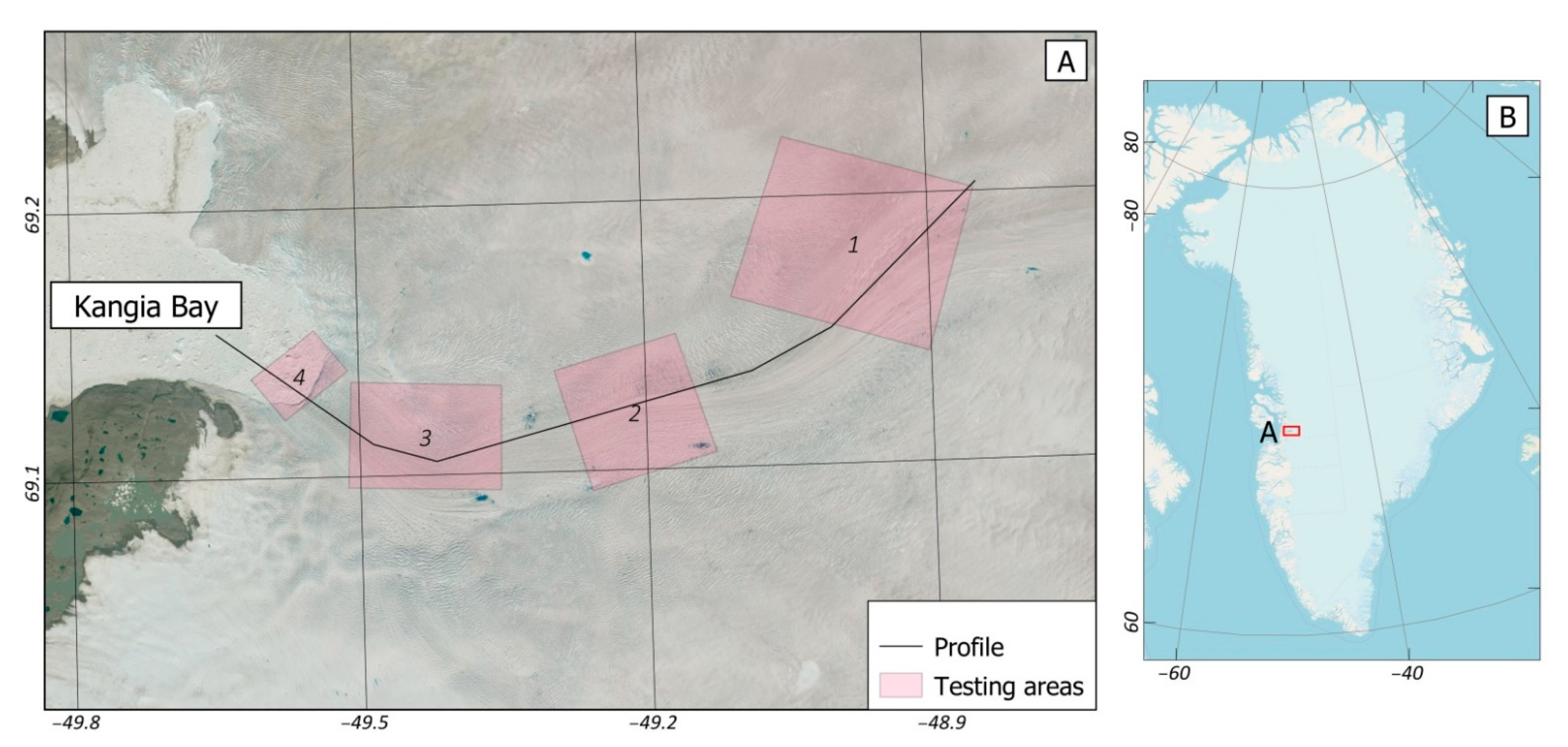
Figure 2.
Data processing for ICEYE and Sentinel-1 missions.

Figure 3.
Distribution of displacements in range and azimuth directions and maximum velocities obtained using radar images from the ICEYE and Sentinel-1 sensors.
Figure 3.
Distribution of displacements in range and azimuth directions and maximum velocities obtained using radar images from the ICEYE and Sentinel-1 sensors.
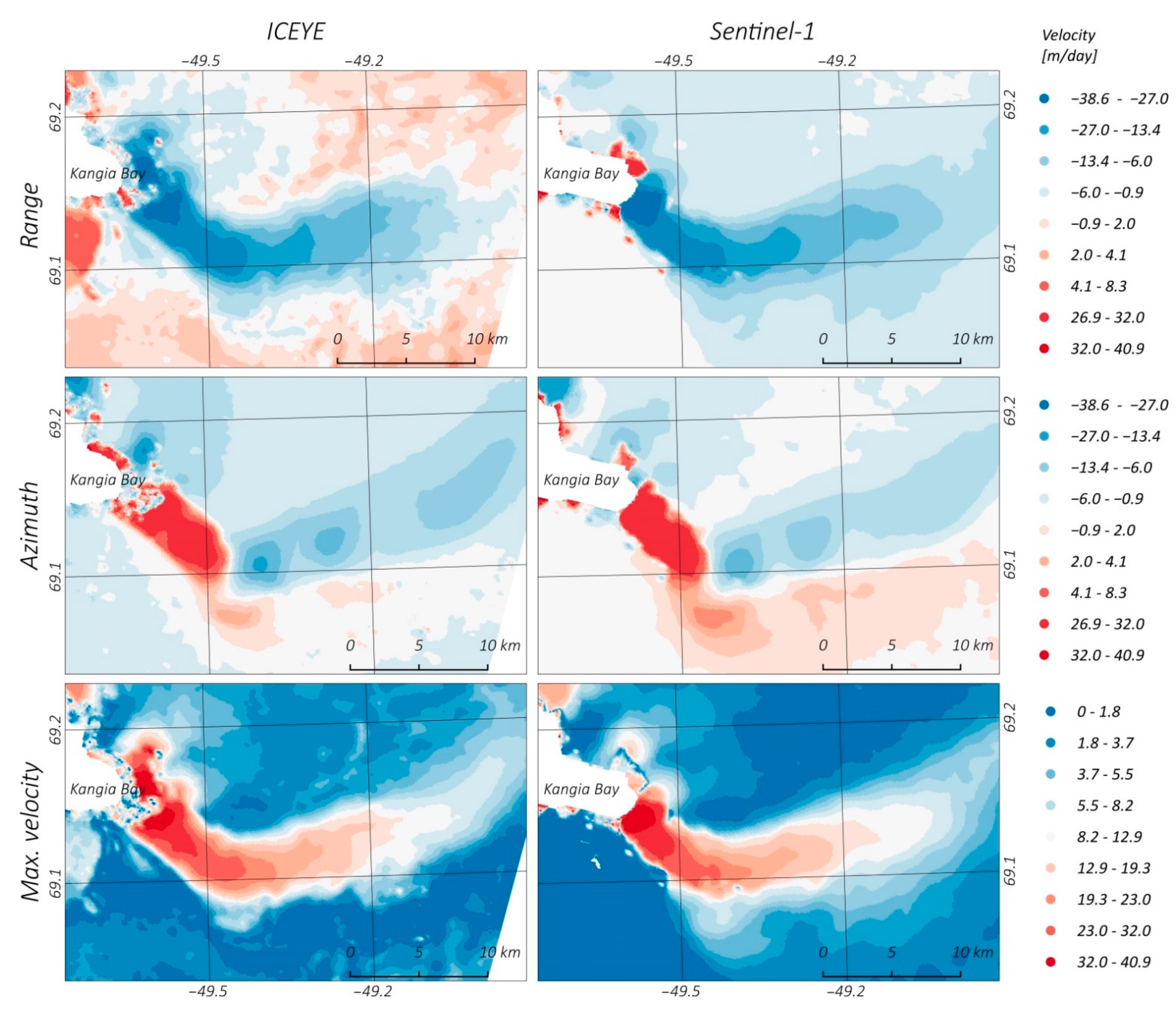
Figure 4.
Areas where detailed comparative analyzes were applied and a field profile. The map shows the maximum velocity of glacier movement obtained based on the ICEYE satellite.
Figure 4.
Areas where detailed comparative analyzes were applied and a field profile. The map shows the maximum velocity of glacier movement obtained based on the ICEYE satellite.
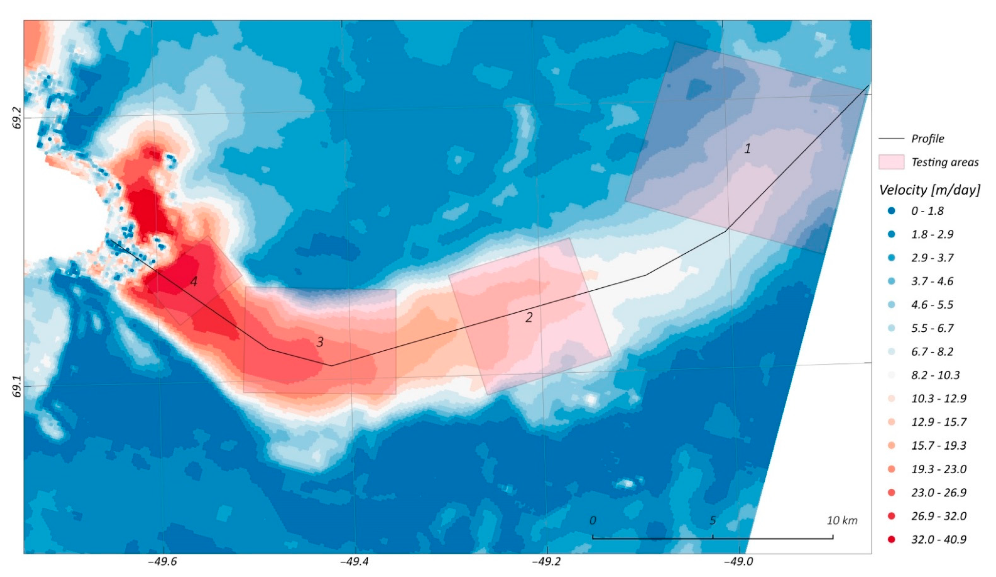
Figure 5.
Correlation plots for selected parts of the glacier for the area in the interior of the glacier (area 1), in area of higher velocities (area 2), in area of high-intensity movements (area 3), in the area of maximum values near the terminus (area 4).
Figure 5.
Correlation plots for selected parts of the glacier for the area in the interior of the glacier (area 1), in area of higher velocities (area 2), in area of high-intensity movements (area 3), in the area of maximum values near the terminus (area 4).
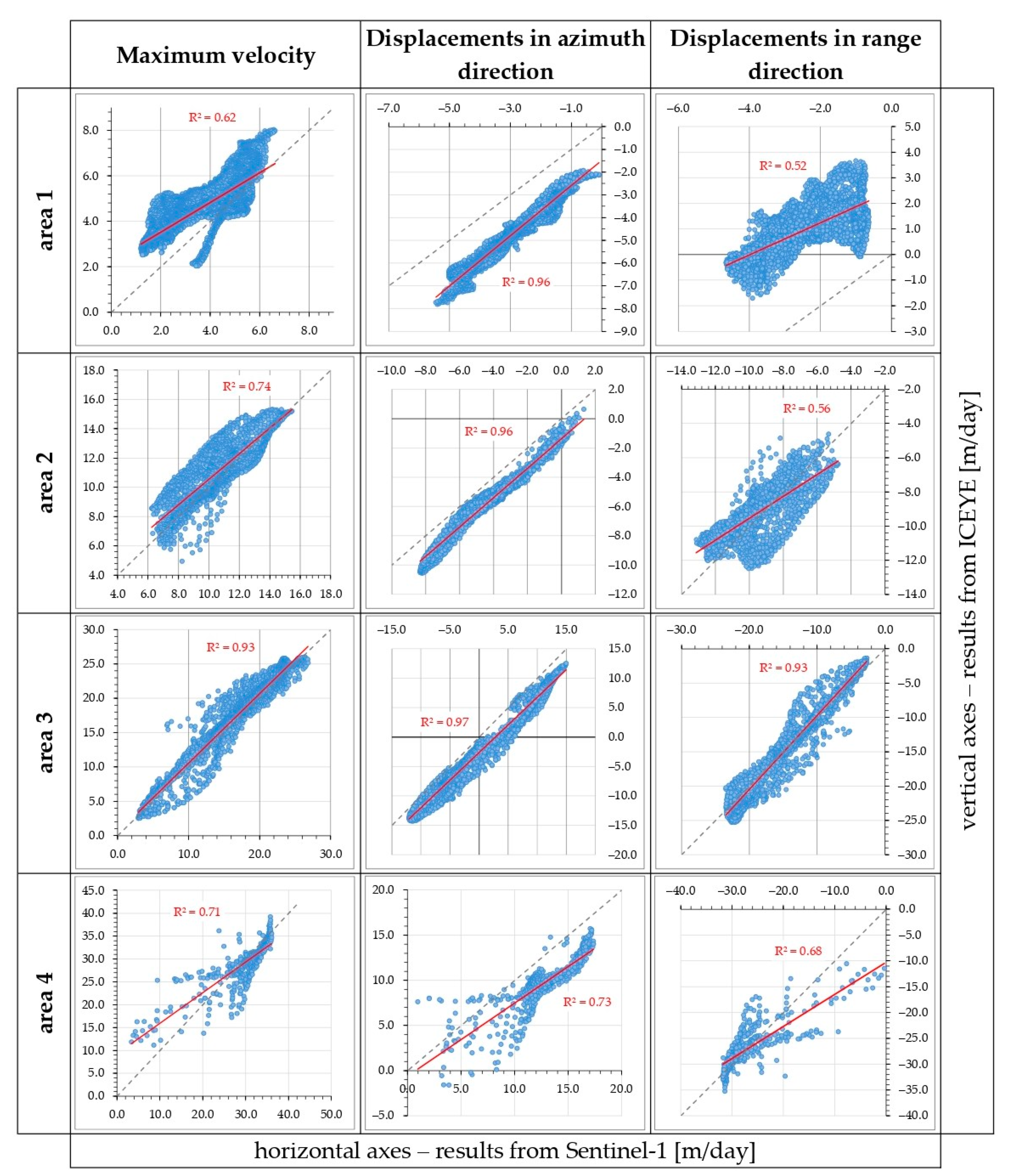
Figure 6.
Velocities along the glacier profile from Sentinel-1 and ICEYE data.

Figure 7.
Amplitude images from radar data acquired on 5 and 9 January 2021 by the ICEYE satellite and 3 and 9 January 2021 by the Sentinel-1 satellite.
Figure 7.
Amplitude images from radar data acquired on 5 and 9 January 2021 by the ICEYE satellite and 3 and 9 January 2021 by the Sentinel-1 satellite.

Table 1.
Specification of the products.
| Date | Sensor | Acquisition Mode | Incident Angle [°] | Heading [°] | Pixel Spacing | Swath Width | Polarization | Orbit Direction |
|---|---|---|---|---|---|---|---|---|
| 3 January | S-1A | Interferometric Wide | 30.3–45.6 | 203.7 | 10 × 10 m | 250 km | HH | desc |
| 5 January | X4 | Stripmap High | 26.9–30.1 | 196.5 | 2.5 × 2.5 m | 30 km | VV | desc |
| 9 January | S-1B | Interferometric Wide | 30.3–45.6 | 203.2 | 10 × 10 m | 250 km | HH | desc |
| 9 January | X7 | Stripmap High | 18.0–22.4 | 198.4 | 2.5 × 2.5 m | 30 km | VV | desc |
Table 2.
Parameters selected for calculations using the offset-tracking technique.
| Parameter | ICEYE | Sentinel-1 |
|---|---|---|
| Max velocity [m/day] | 50 | 50 |
| Registration window width [pxl] | 128 | 128 |
| Registration window height [pxl] | 128 | 128 |
| Grid azimuth spacing [pxl] | 40 | 10 |
| Grid range spacing [pxl] | 40 | 10 |
Publisher’s Note: MDPI stays neutral with regard to jurisdictional claims in published maps and institutional affiliations. |
© 2021 by the authors. Licensee MDPI, Basel, Switzerland. This article is an open access article distributed under the terms and conditions of the Creative Commons Attribution (CC BY) license (https://creativecommons.org/licenses/by/4.0/).
Share and Cite
MDPI and ACS Style
Łukosz, M.A.; Hejmanowski, R.; Witkowski, W.T. Evaluation of ICEYE Microsatellites Sensor for Surface Motion Detection—Jakobshavn Glacier Case Study. Energies 2021, 14, 3424. https://doi.org/10.3390/en14123424
AMA Style
Łukosz MA, Hejmanowski R, Witkowski WT. Evaluation of ICEYE Microsatellites Sensor for Surface Motion Detection—Jakobshavn Glacier Case Study. Energies. 2021; 14(12):3424. https://doi.org/10.3390/en14123424
Chicago/Turabian StyleŁukosz, Magdalena A., Ryszard Hejmanowski, and Wojciech T. Witkowski. 2021. "Evaluation of ICEYE Microsatellites Sensor for Surface Motion Detection—Jakobshavn Glacier Case Study" Energies 14, no. 12: 3424. https://doi.org/10.3390/en14123424
Note that from the first issue of 2016, this journal uses article numbers instead of page numbers. See further details here.