
Customized yet Standardized Temperature Derivatives: A Non-Parametric Approach with Suitable Basis Selection for Ensuring Robustness


Abstract
1. Introduction
2. Overview of Background Data
3. Minimum Variance Hedging Problem
3.1. Optimal Futures Contract Volume Calculation Problem
3.2. Optimal Derivative Payoff Calculation Problem
3.3. Spline Function Estimation Procedure
3.3.1. Univariate Smoothing Spline Function
- “Cubic spline”: It is one of the most popular basis functions and is defined based on the third order “truncated power basis functions.” In other words, it is expressed by cubic polynomials, and each piecewise polynomial smoothly connects at each knot (i.e., the value, the first derivative, and the second derivative are continuous; see Appendix C.1 for the concrete formulas).
- “Cyclic cubic spline”: It has a basis function that is defined to be smoothly connected not only at each knot, but also at the start and end points of the domain (see Appendix C.2 for the concrete formulas). For this reason, it is suitable for robustly estimating the trend of periodic data.
- “P-spline”: While using B-spline basis [25] (which is based on “a special parametrization of a cubic spline” [26]), P-spline uses the unique penalty term called “discrete penalty” [21]. Unlike the other basis functions having “continuous penalties” with “integral squared curvature,” as shown in (5), P-spline penalizes the changes in discrete coefficients of adjacent bases of B-spline (see [21] for the formula of penalty term). Initially, B-spline bases are arranged so that adjacent bell-shape curves overlap each other (e.g., see “Figure 1” of [21]); therefore, even though the discrete penalty is imposed for coefficients of the bases, smoothness is ensured, as in the case of continuous penalties.
- “Thin plate spline”: Also called “radial basis functions,” the basis of the thin plate spline depends only on the distance (norm) from each control point rather than the coordinates for each dimension. Therefore, unlike the previous three bases, the “thin plate spline” does not have “knots” as connection points (see [20,23] for more detail).
3.3.2. Multivariate Smoothing Spline Function
3.3.2.1. Tensor Product Smoothing (Tensor Product Spline)
3.3.2.2. Isotropic Smoothing
4. Construction of Hedging Models
4.1. Base Model Consisting of Fuel Price and Calendar Trend
4.2. Temperature Futures
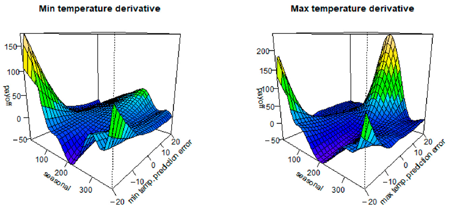
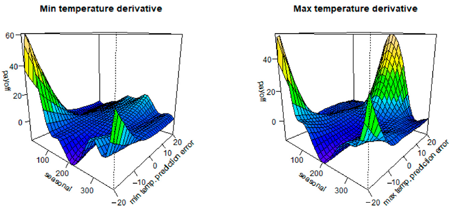
4.3. Temperature Derivatives Estimated by the Tensor Product Spline
4.4. Temperature Derivatives for the Squared Prediction Error
5. Empirical Analysis
- (a)
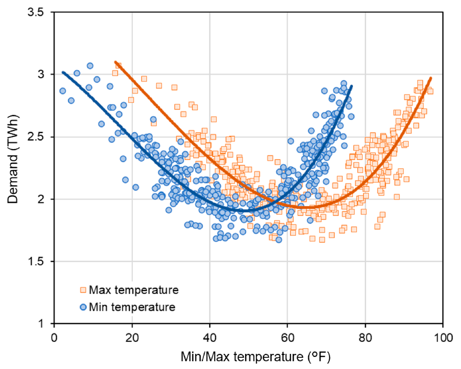
- Demand (TWh): the hourly load of the entire PJM-RTO [31].
- (b)
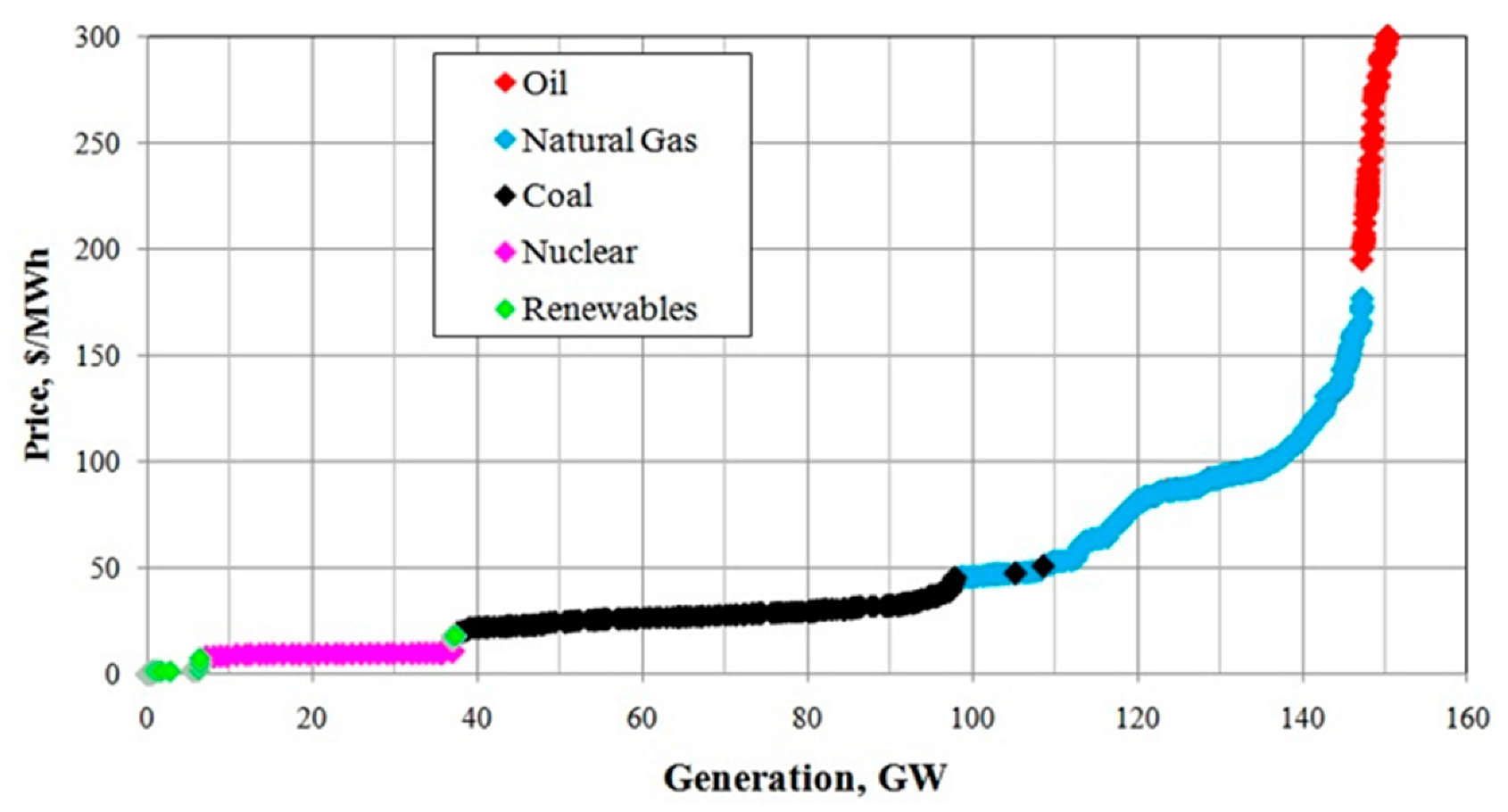
- Electricity price (USD/MWh): day-ahead hourly spot price of PJM-RTO [31].
- (c)
- Maximum and minimum temperatures , : population-weighted average of four main cities (Philadelphia, Pittsburgh, Baltimore, and Newark) published by the National Oceanic and Atmospheric Administration (NOAA) [32].
- (d)
- Henry Hub natural gas price (USD/million BTU): historical daily HH spot price FOB [33].
5.1. Empirical Analysis by Business Risk Models
5.1.1. Trend Estimation of Hedge Models
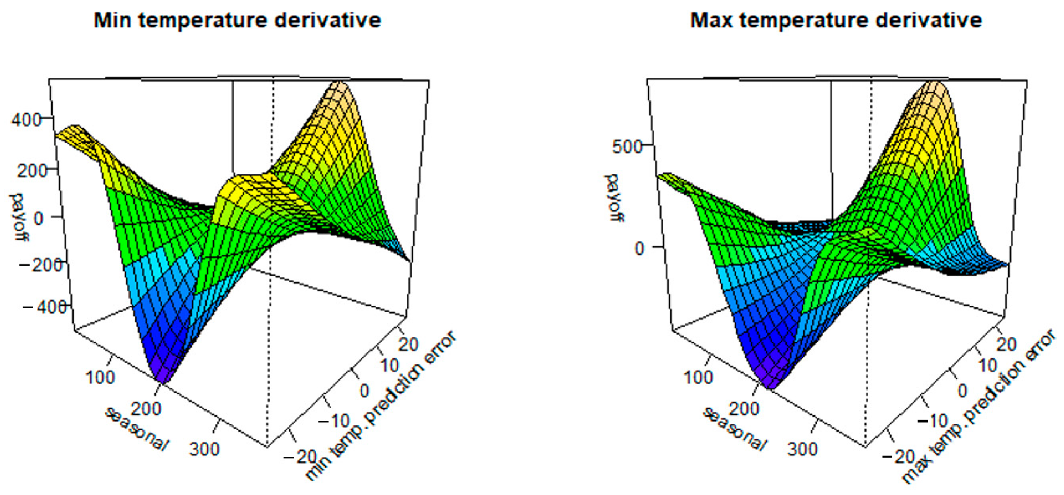
5.1.1.1. Optimal Payoff Function of the Temperature Derivatives
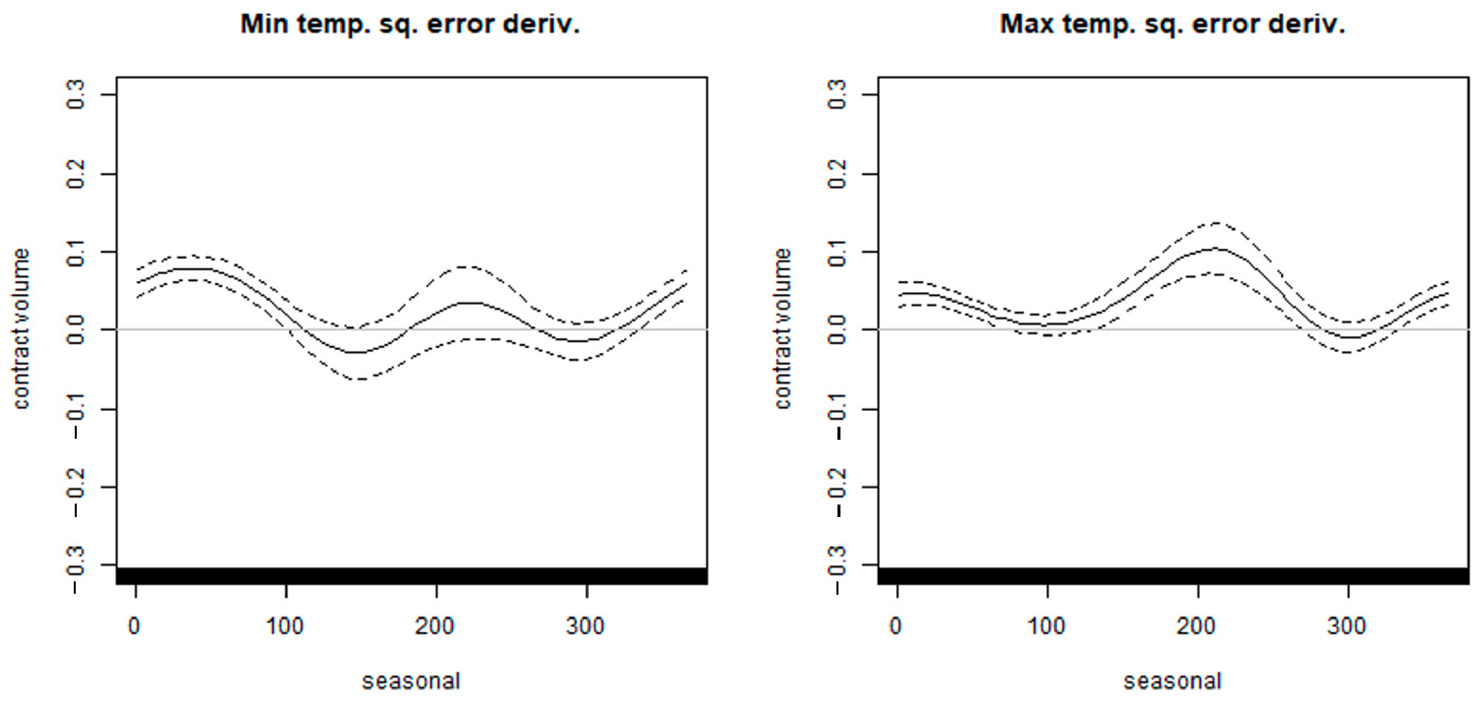
5.1.1.2. Optimal Contract Volume of the Squared Temperature Prediction Error Derivatives
5.1.2. Measurement of Hedge Effects
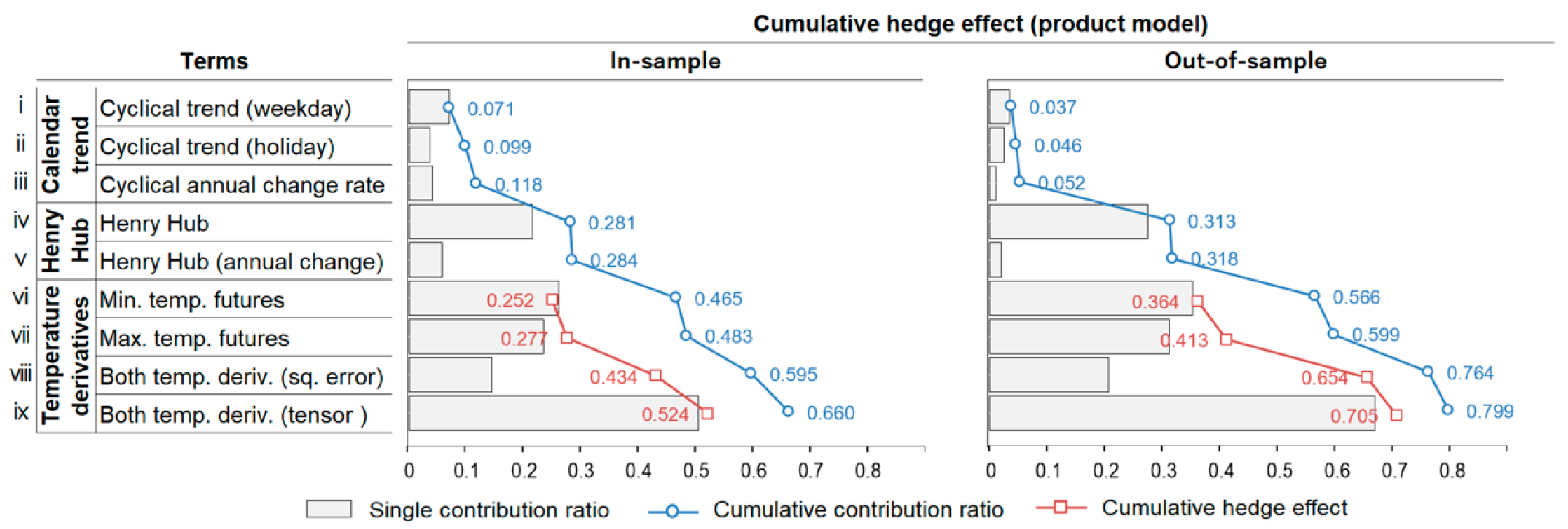
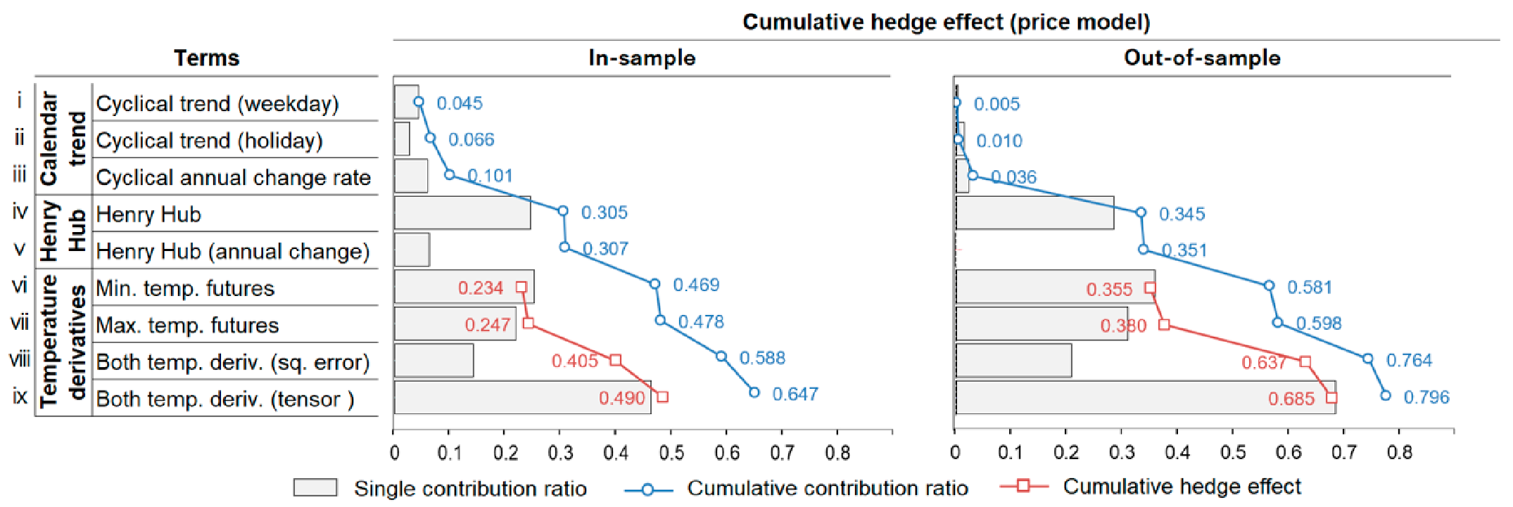
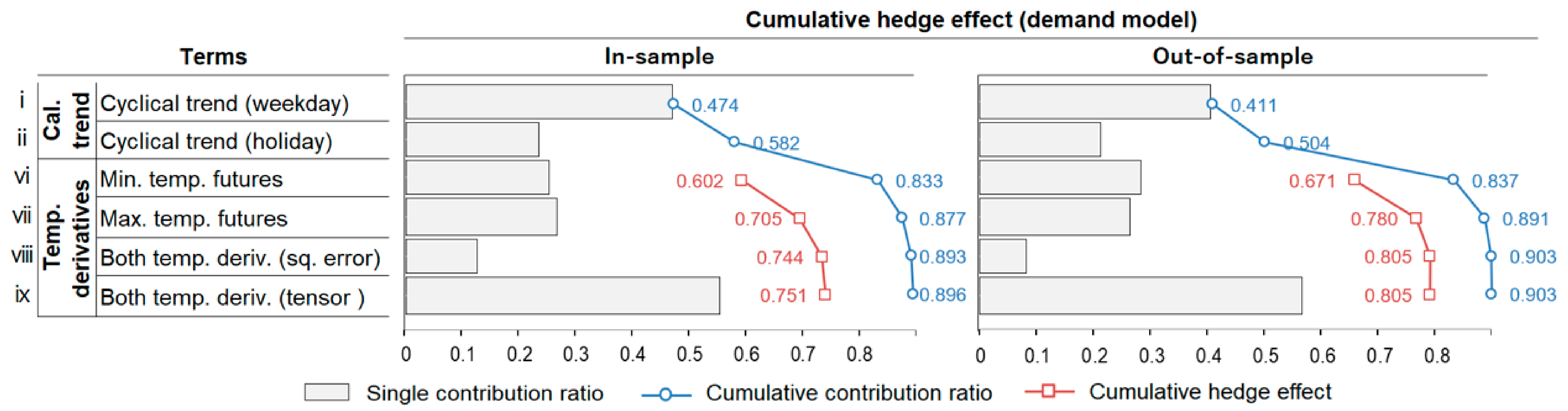
5.1.2.1. Cumulative/Individual Hedge Effects by Derivatives
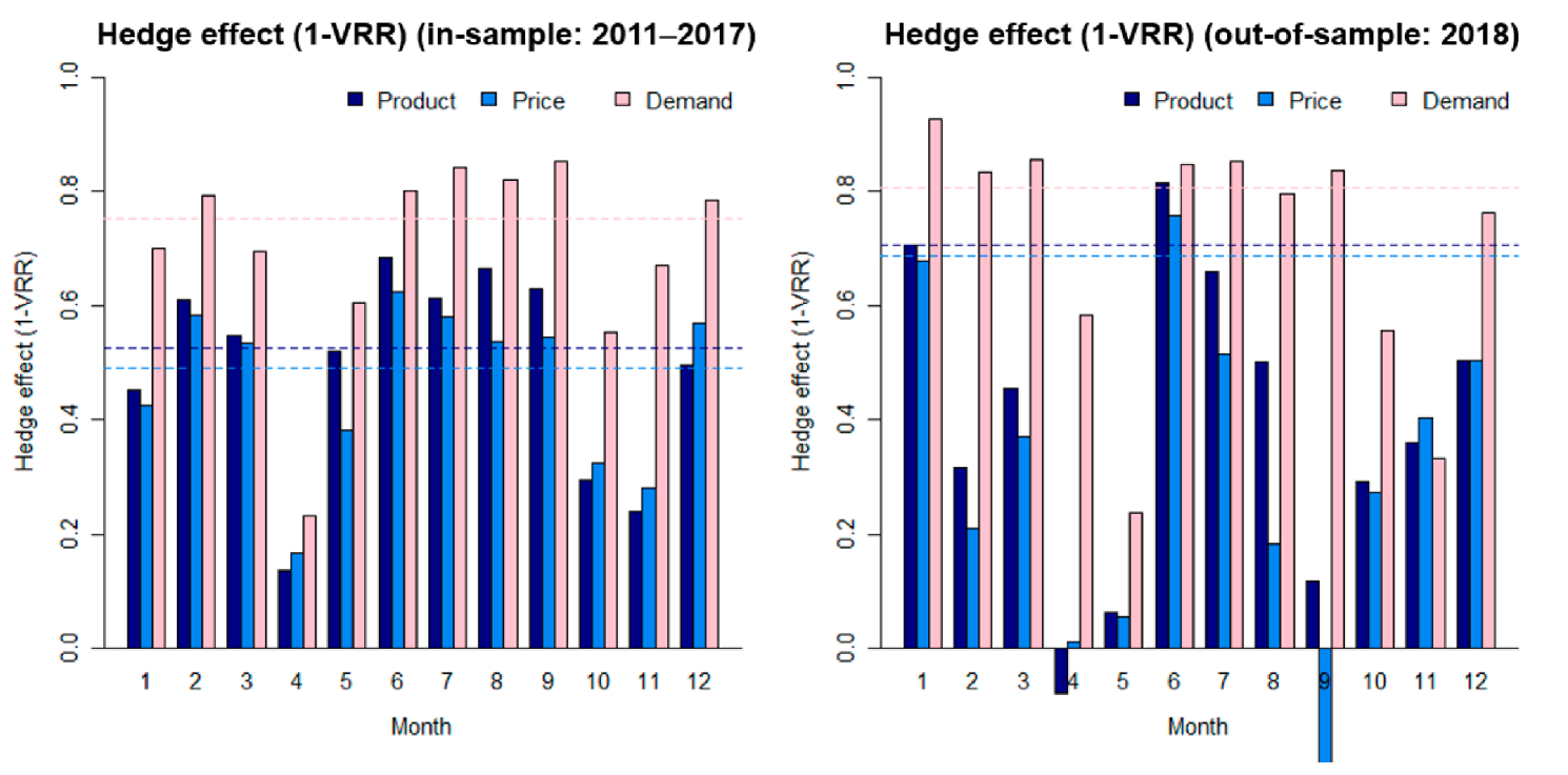
5.1.2.2. Monthly Hedge Effect
5.2. Comparison between Basis Functions
6. Conclusions
- The nonlinearity of the temperature derivative payoffs by the business risk model is strong in the product model and the price model, and relatively weak in the demand model.
- Reflecting this, the non-parametrically-priced derivative payoff function, which can flexibly express strong nonlinearity, has the highest hedge effect on the product model and the price model.
- On the contrary, for the demand model, the hedge effect of the non-parametric derivatives does not exceed that of the standard derivative on the squared temperature prediction error; hence, the squared error derivatives may be superior in that it allows for liquid trading.
- When estimating the series of trends existing in the hedge models, using the P-spline or the cyclic cubic spline instead of the thin plate spline or cubic spline set as the default in the R “mgcv” package can secure the robustness of the models; as a result, the out-of-sample hedge effect may be significantly improved.
- The improvement of the hedge effect by appropriate basis selection is larger for the product and price models than for the demand model. This means that the stronger the nonlinearity in the model, the more critical the basis selection that can robustly express the inherent trends of the data.
Author Contributions
Funding
Conflicts of Interest
Nomenclature
| Date | |
| Hour | |
| Sales revenue (or procurement cost) of an electric utility | |
| Demand | |
| Spot price | |
| Henry Hub natural gas price | |
| Temperature | |
| Maximum/Minimum temperature | |
| Payoff of the temperature futures (temperature prediction error) | |
| Payoff of the squared prediction error derivative on temperature | |
| Payoff of the temperature derivative estimated by tensor product spline function | |
| Contract volume of discount bonds | |
| Contract volume of HH futures | |
| Contract volume of the temperature futures | |
| Contract volume of the squared prediction error derivatives on temperature | |
| Residual term (hedging error of derivative portfolio] | |
| Smoothing parameter | |
| A set of smoothing spline functions with smoothing parameter | |
| Spline function | |
| Penalty term of penalized residual sum of squares | |
| Basis functions of spline function | |
| Coefficients of the basis functions |
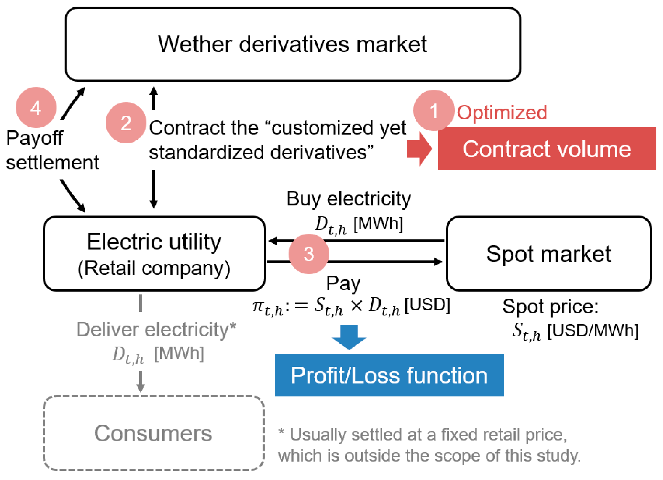
Appendix A. Transaction Flow of “Customized Yet Standardized” Derivatives
- The electric utility optimizes the contract volume (such as and ) of the standard derivatives for each future delivery date based on the past profit/loss function (for the retailer in the figure, it is procurement cost ).
- The utility makes a contract (transaction) of the temperature derivatives of the volume calculated in 1. in the derivative market. At this time, no premium payment is made.
- The utility purchases electricity at the spot market and pays the corresponding procurement cost (or records the cost in its account books) on the day before the delivery date of electricity.
- The utility receives (or pays) a payoff of temperature derivatives calculated based on the measured temperature on the delivery day of electricity. (Since this payoff is greatly linked to the procurement cost of 3., the net cash flow, which is the sum of 3. and 4., will be less volatile than the original cash flow of 3.)

Appendix B. Separation of Deterministic Trends by ANOVA Decomposition
Appendix C. Basis Functions of the Cubic Spline and the Cyclic Cubic Spline
Appendix C.1. Cubic Spline Function
Appendix C.2. Cyclic Cubic Spline Function
Appendix D. Monthly RMSE and Daily Fitting Curves
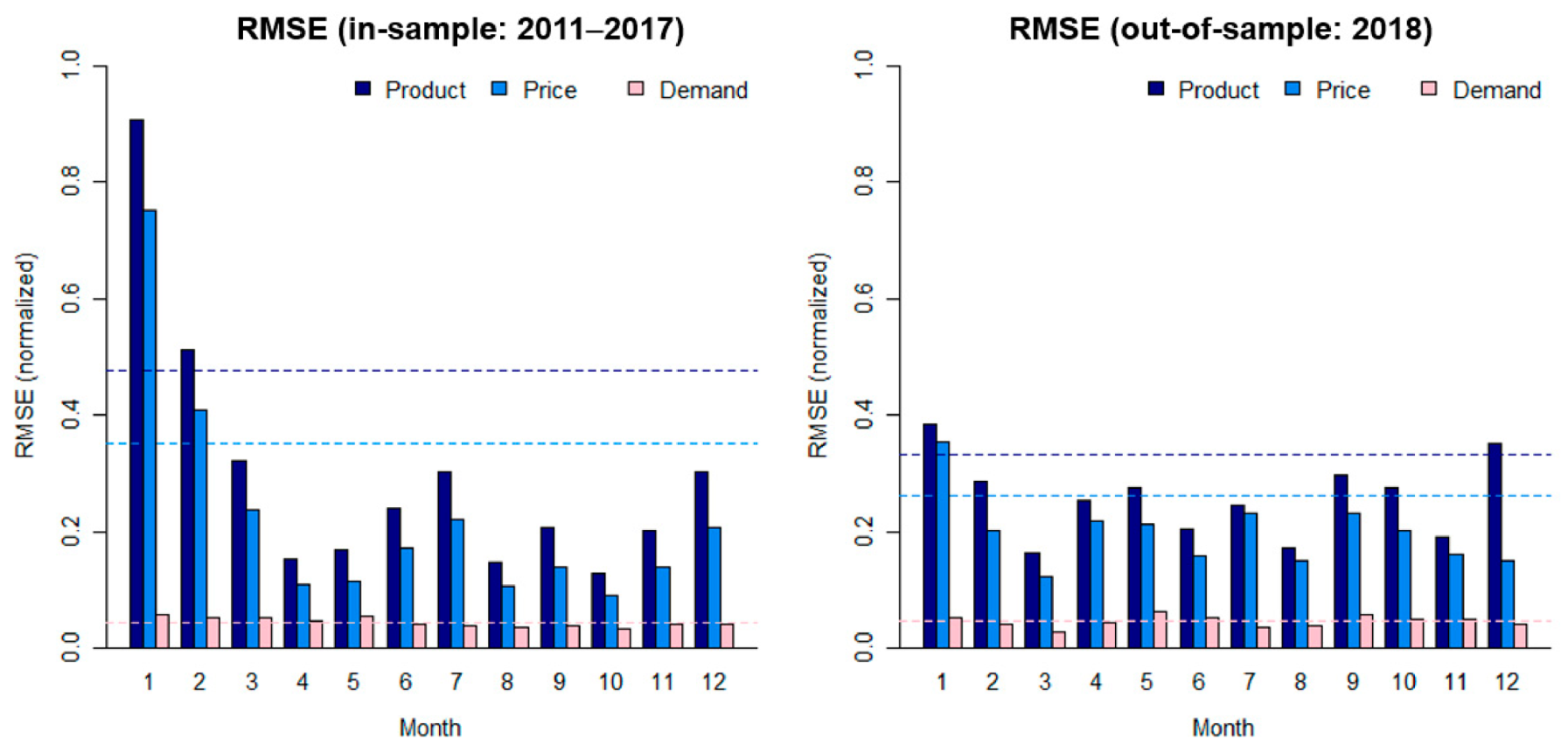
Appendix D.1. Monthly RMSE

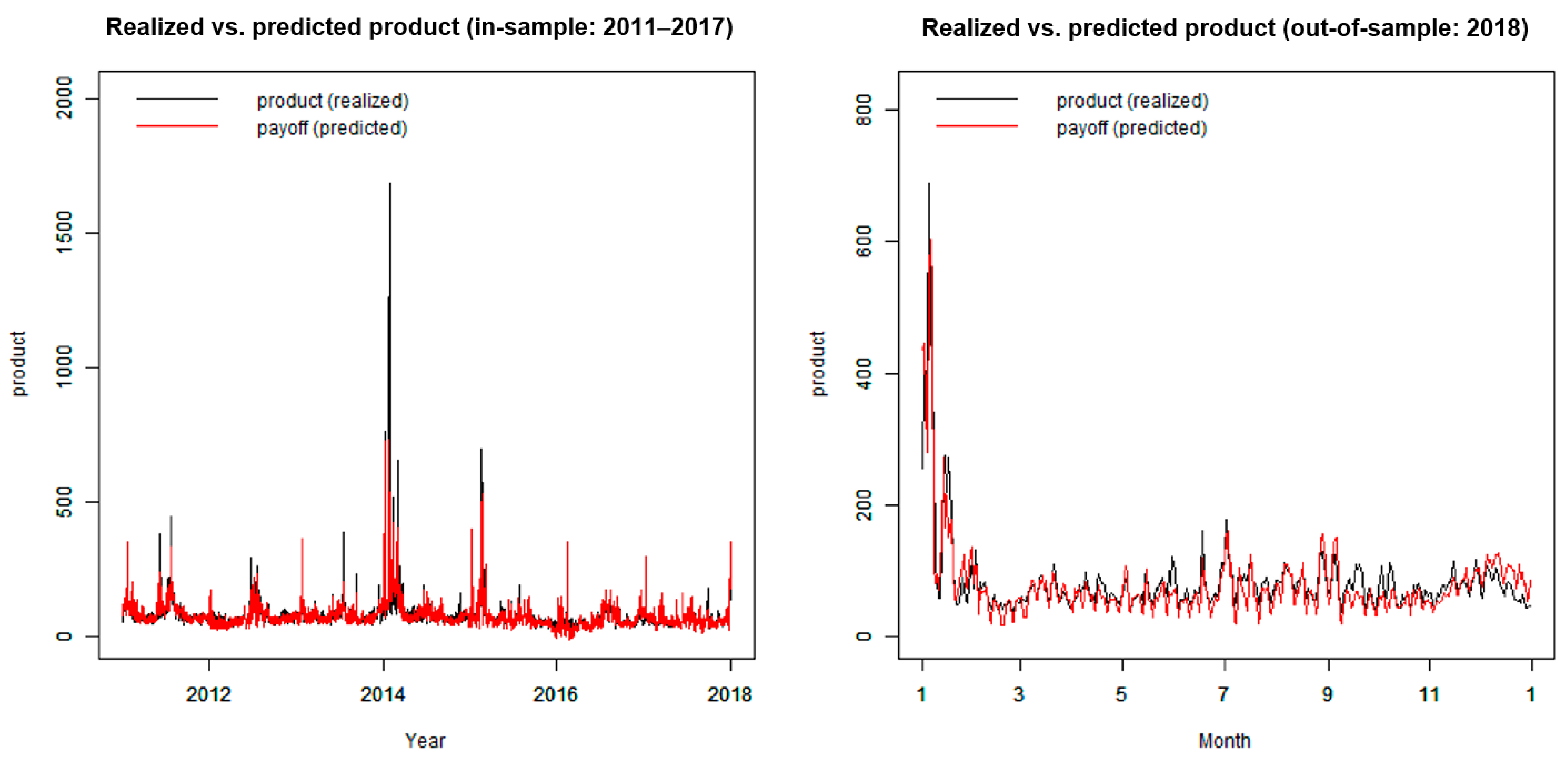
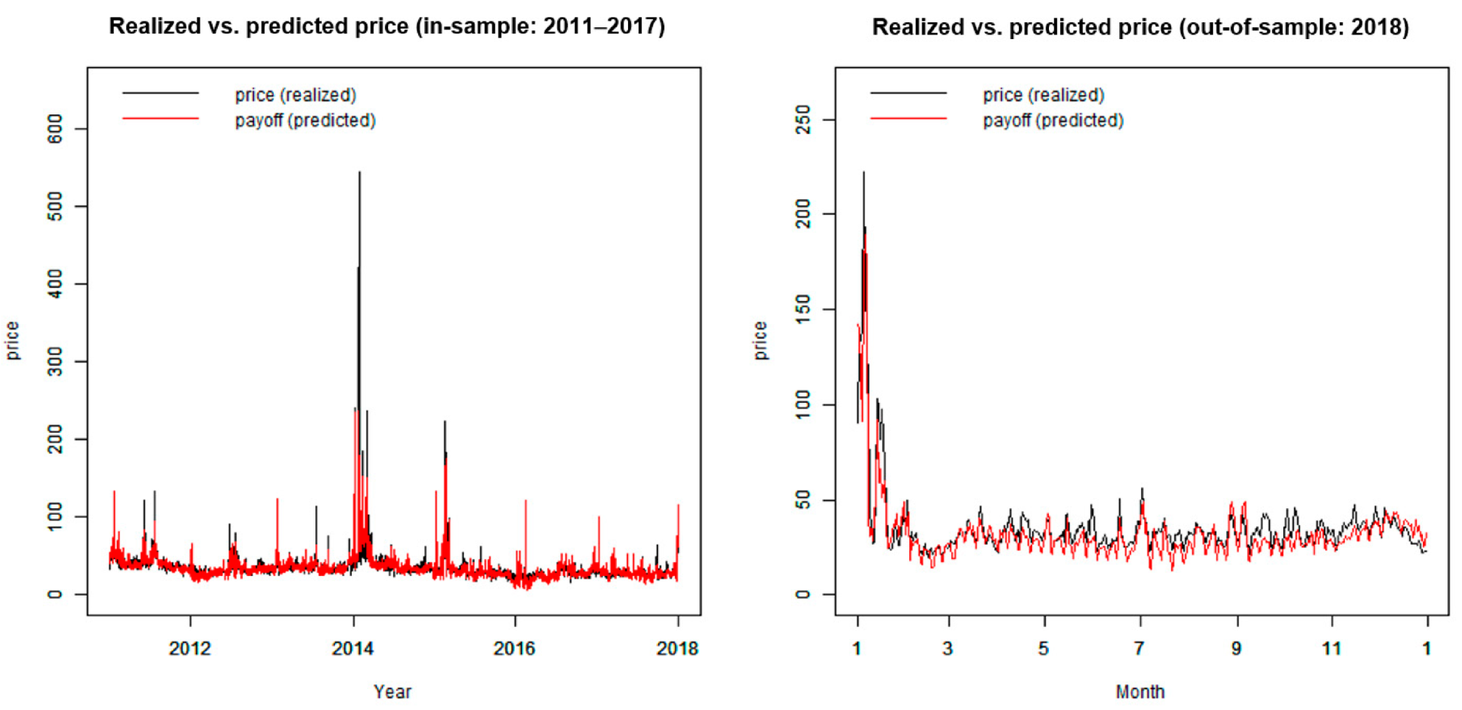
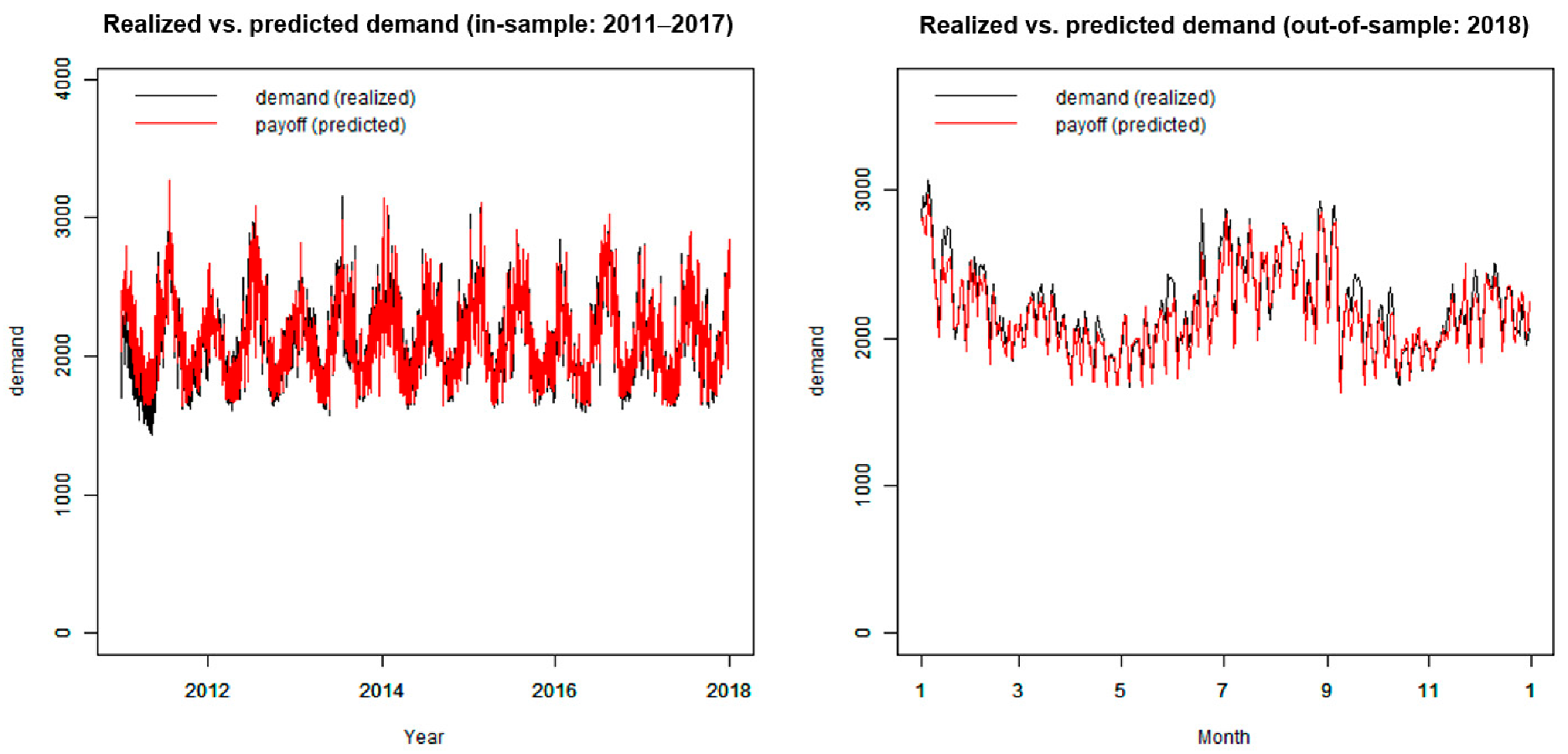
Appendix D.2. Daily Fitting Curves


References
- Lee, Y.; Oren, S.S. An equilibrium pricing model for weather derivatives in a multi-commodity setting. Energy Econ. 2009, 31, 702–713. [Google Scholar] [CrossRef]
- Lee, Y.; Oren, S.S. A multi-period equilibrium pricing model of weather derivatives. Energy Syst. 2010, 1, 3–30. [Google Scholar] [CrossRef]
- Bhattacharya, S.; Gupta, A.; Kar, K.; Owusu, A. Risk management of renewable power producers from co-dependencies in cash flows. Eur. J. Oper. Res. 2020, 283, 1081–1093. [Google Scholar] [CrossRef]
- Davis, M. Pricing weather derivatives by marginal value. Quant. Financ. 2001, 1, 305–308. [Google Scholar] [CrossRef]
- Platen, E.; West, J. A Fair Pricing Approach to Weather Derivatives. Asia Pac. Financ. Mark. 2004, 11, 23–53. [Google Scholar] [CrossRef]
- Brockett, P.L.; Wang, M.; Yang, C.; Zou, H. Portfolio Effects and Valuation of Weather Derivatives. Financ. Rev. 2006, 41, 55–76. [Google Scholar] [CrossRef]
- Kanamura, T.; Ohashi, K. Pricing summer day options by good-deal bounds. Energy Econ. 2009, 31, 289–297. [Google Scholar] [CrossRef]
- Yamada, Y. Valuation and hedging of weather derivatives on monthly average temperature. J. Risk 2007, 10, 101–125. [Google Scholar] [CrossRef]
- Yamada, Y. Simultaneous optimization for wind derivatives based on prediction errors. In Proceedings of the 2008 American Control Conference, Seattle, WA, USA, 11–13 June 2008; pp. 350–355. [Google Scholar]
- Yamada, Y. Optimal Hedging of Prediction Errors Using Prediction Errors. Asia Pac. Financ. Mark. 2008, 15, 67–95. [Google Scholar] [CrossRef]
- Matsumoto, T.; Yamada, Y. Cross Hedging Using Prediction Error Weather Derivatives for Loss of Solar Output Prediction Errors in Electricity Market. Asia Pac. Financ. Mark. 2018, 26, 211–227. [Google Scholar] [CrossRef]
- Yamada, Y. Simultaneous hedging of demand and price by temperature and power derivative portfolio: Consideration of periodic correlation using GAM with cross variable. In Proceedings of the 50th JAFEE Winter Conference, Tokyo, Japan, 22–23 February 2019. [Google Scholar]
- Matsumoto, T.; Yamada, Y. Hedging strategies for solar power businesses in electricity market using weather derivatives. In Proceedings of the 2019 IEEE 2nd International Conference on Renewable Energy and Power Engineering (REPE), Toronto, ON, Canada, 2–4 November 2019; pp. 236–240. [Google Scholar]
- Matsumoto, T.; Yamada, Y. Simultaneous hedging strategy for price and volume risks in electricity businesses using energy and weather derivatives. Energy Econ. 2021, 95, 105101. [Google Scholar] [CrossRef]
- Hastie, T.; Tibshirani, R. Generalized Additive Models; Chapman & Hall: Boca Raton, FL, USA, 1990. [Google Scholar]
- EMSC, Electricity and Gas Market Surveillance Commission. Current Status of Activation of Wholesale Power Trading, 21st Institutional Design Special Meeting Secretariat Submission Materials. 2017. Available online: https://www.emsc.meti.go.jp/activity/emsc_system/pdf/021_04_00.pdf (accessed on 11 April 2021).
- Wood, S.N. Package mgcv v. 1.8-34. Available online: https://cran.r-project.org/web/packages/mgcv/mgcv.pdf (accessed on 11 April 2021).
- Matsumoto, T. Forecast Based Risk Management for Electricity Trading Market. Ph.D. Thesis, University of Tsukuba, Tokyo, Japan, 2020. [Google Scholar]
- Hastie, T.; Tibshirani, R.; Friedman, J. The Elements of Statistical Learning: Data Mining, Inference, and Prediction; Springer: Berlin/Heidelberg, Germany, 2009. [Google Scholar]
- Wood, S.N. Thin plate regression splines. J. R. Stat. Soc. Ser. B Stat. Methodol. 2003, 65, 95–114. [Google Scholar] [CrossRef]
- Eilers, P.H.C.; Marx, B.D. Flexible smoothing with B-splines and penalties. Stat. Sci. 1996, 11, 89–121. [Google Scholar] [CrossRef]
- Eilers, P.H.; Marx, B.D. Practical Smoothing: The Joys of P-Splines; Cambridge University Press: Cambridge, MA, USA, 2021. [Google Scholar]
- Wood, S.N. Generalized Additive Models: An Introduction with R, 2nd ed.; Chapman & Hall: Boca Raton, FL, USA, 2017. [Google Scholar]
- Efron, B.; Stein, C. The Jackknife Estimate of Variance. Ann. Stat. 1981, 9, 586–596. [Google Scholar] [CrossRef]
- De Boor, C. A Practical Guide to Splines; Springer: New York, NY, USA, 1978; Volume 27, p. 325. [Google Scholar]
- Perperoglou, A.; Sauerbrei, W.; Abrahamowicz, M.; Schmid, M. A review of spline function procedures in R. BMC Med. Res. Methodol. 2019, 19, 1–16. [Google Scholar] [CrossRef]
- McCulloch, J.; Ignatieva, K. Intra-day Electricity Demand and Temperature. Energy J. 2020, 41. [Google Scholar] [CrossRef]
- Duchon, J. Splines minimizing rotation-invariant semi-norms in Sobolev spaces. In Constructive Theory of Functions of Several Variables; Springer: Berlin/Heidelberg, Germany, 1977; pp. 85–100. [Google Scholar]
- Wood, S.N.; Bravington, M.V.; Hedley, S.L. Soap film smoothing. J. R. Stat. Soc. Ser. B Stat. Methodol. 2008, 70, 931–955. [Google Scholar] [CrossRef]
- Yamada, Y.; Makimoto, N.; Takashima, R. JEPX price predictions using GAMs and estimations of volume-price functions. JAFEE J. 2015, 14, 8–39. [Google Scholar]
- PJM Data Miner 2. Available online: http://dataminer2.pjm.com/ (accessed on 25 June 2019).
- NOAA Climate Data Online Search. Available online: https://www.ncdc.noaa.gov/cdo-web/search (accessed on 25 June 2019).
- EIA Henry Hub Natural Gas Spot Price. Available online: https://www.eia.gov/dnav/ng/hist/rngwhhdd.htm (accessed on 25 June 2019).
- Thompson, T.; Webber, M.; Allen, D.T. Air quality impacts of using overnight electricity generation to charge plug-in hybrid electric vehicles for daytime use. Environ. Res. Lett. 2009, 4, 014002. [Google Scholar] [CrossRef]
- Campbell, J.Y.; Thompson, S.B. Predicting Excess Stock Returns Out of Sample: Can Anything Beat the Historical Average? Rev. Financ. Stud. 2007, 21, 1509–1531. [Google Scholar] [CrossRef]
- Aguilera, A.; Aguilera-Morillo, M. Comparative study of different B-spline approaches for functional data. Math. Comput. Model. 2013, 58, 1568–1579. [Google Scholar] [CrossRef]
- PJM. Analysis of Operational Events and Market Impacts during the January 2014 Cold Weather Events. Available online: https://www.hydro.org/wp-content/uploads/2017/08/PJM-January-2014-report.pdf (accessed on 11 April 2021).


| Business Risk Model | In Sample | Out-of-Sample | |||||||||||||
|---|---|---|---|---|---|---|---|---|---|---|---|---|---|---|---|
| Cumulative Contribution Ratio | Cumulative Hedge Effect | Cumulative Contribution Ratio | Cumulative Hedge Effect | ||||||||||||
| tp/cr | ps | cc | tp/cr | ps | cc | tp/cr | ps | cc | tp/cr | ps | cc | Δ (to tp/cr) | |||
| ps | cc | ||||||||||||||
| Product | vi | 0.480 | 0.477 | 0.465 | 0.267 | 0.262 | 0.252 | 0.521 | 0.546 | 0.566 | 0.238 | 0.289 | 0.364 | 21% | 53% |
| vii | 0.495 | 0.492 | 0.483 | 0.289 | 0.283 | 0.277 | 0.548 | 0.571 | 0.599 | 0.281 | 0.329 | 0.413 | 17% | 47% | |
| viii | 0.601 | 0.598 | 0.595 | 0.438 | 0.433 | 0.434 | 0.720 | 0.722 | 0.764 | 0.555 | 0.565 | 0.654 | 2% | 18% | |
| ix | 0.660 | 0.641 | 0.660 | 0.520 | 0.493 | 0.524 | 0.762 | 0.788 | 0.799 | 0.621 | 0.668 | 0.705 | 8% | 13% | |
| Price | vi | 0.484 | 0.483 | 0.469 | 0.246 | 0.244 | 0.234 | 0.545 | 0.568 | 0.581 | 0.248 | 0.290 | 0.355 | 17% | 43% |
| vii | 0.494 | 0.491 | 0.478 | 0.259 | 0.257 | 0.247 | 0.564 | 0.585 | 0.598 | 0.278 | 0.318 | 0.380 | 14% | 37% | |
| viii | 0.596 | 0.592 | 0.588 | 0.409 | 0.404 | 0.405 | 0.731 | 0.733 | 0.764 | 0.555 | 0.561 | 0.637 | 1% | 15% | |
| ix | 0.647 | 0.633 | 0.647 | 0.484 | 0.463 | 0.490 | 0.781 | 0.782 | 0.796 | 0.637 | 0.642 | 0.685 | 1% | 8% | |
| Demand | vi | 0.837 | 0.826 | 0.833 | 0.607 | 0.589 | 0.602 | 0.835 | 0.837 | 0.837 | 0.668 | 0.667 | 0.671 | 0% | 0% |
| vii | 0.881 | 0.870 | 0.877 | 0.712 | 0.694 | 0.705 | 0.887 | 0.894 | 0.891 | 0.772 | 0.783 | 0.780 | 1% | 1% | |
| viii | 0.896 | 0.888 | 0.893 | 0.748 | 0.735 | 0.744 | 0.902 | 0.907 | 0.903 | 0.802 | 0.810 | 0.805 | 1% | 0% | |
| ix | 0.898 | 0.891 | 0.896 | 0.753 | 0.744 | 0.751 | 0.903 | 0.905 | 0.903 | 0.804 | 0.804 | 0.805 | 0% | 0% | |
Publisher’s Note: MDPI stays neutral with regard to jurisdictional claims in published maps and institutional affiliations. |
© 2021 by the authors. Licensee MDPI, Basel, Switzerland. This article is an open access article distributed under the terms and conditions of the Creative Commons Attribution (CC BY) license (https://creativecommons.org/licenses/by/4.0/).
Share and Cite
Matsumoto, T.; Yamada, Y. Customized yet Standardized Temperature Derivatives: A Non-Parametric Approach with Suitable Basis Selection for Ensuring Robustness. Energies 2021, 14, 3351. https://doi.org/10.3390/en14113351
Matsumoto T, Yamada Y. Customized yet Standardized Temperature Derivatives: A Non-Parametric Approach with Suitable Basis Selection for Ensuring Robustness. Energies. 2021; 14(11):3351. https://doi.org/10.3390/en14113351
Chicago/Turabian StyleMatsumoto, Takuji, and Yuji Yamada. 2021. "Customized yet Standardized Temperature Derivatives: A Non-Parametric Approach with Suitable Basis Selection for Ensuring Robustness" Energies 14, no. 11: 3351. https://doi.org/10.3390/en14113351
APA StyleMatsumoto, T., & Yamada, Y. (2021). Customized yet Standardized Temperature Derivatives: A Non-Parametric Approach with Suitable Basis Selection for Ensuring Robustness. Energies, 14(11), 3351. https://doi.org/10.3390/en14113351