Towards Renewable-Dominated Power Systems Considering Long-Term Uncertainties: Case Study of Las Palmas

Abstract

In this paper, we analyze the generation, storage and transmission expansion of the isolated power system of Las Palmas (Spain) for 2050. This power system comprises two isolated systems: Lanzarote-Fuerteventura and Gran Canaria. The generating, storage and transmission capacity to be built is determined by solving a two-stage stochastic investment model taking into account different long-term uncertain parameters: investment costs of immature technologies of power production and storage, annual demand growth, number of electric vehicles, rooftop solar penetration and natural gas prices. The possibility of linking together the isolated power systems of Lanzarote-Fuerteventura and Gran Canaria for reaching a higher penetration of renewable units is also considered. The operation of the power system is simulated by considering the day-ahead energy and reserve capacity markets. The variability of the hourly available wind and solar power, and the demand level are modeled by using a set of characteristic days to represent the target year. The performance of the resulting power system is assessed by conducting an out-of-sample analysis using the AC model of the power system. The numerical results show that a future configuration of Las Palmas power system mainly based on solar and wind power units can be achieved with the support of gas units and storage.

1. Introduction

The design of future power systems is more challenging than ever for a variety of reasons. The highly demanding decarbonization targets to achieve by the electricity sector in the forthcoming years are pushing renewable generation technologies to replace conventional ones. For instance, a reduction of 80–95% of greenhouse gas emissions in 2050 compared to the 1990 levels has been established by the European Commission in [1]. This ambitious benchmark will require, among other measures, that the CO${}_2$ emissions of the power sector be almost null. However, considering that the availability and dispatchability of the production of most renewable power plants is much lower than those of traditional generating units, a massive incorporation of renewable plants can have sensible consequences on the day to day operation of future power systems. The possibility of increasing the energy storage capacity will be key to facilitate the integration of renewable power units. In this manner, part of the exceeding energy in periods with high renewable production may be used afterwards when the available renewable production be lower. To date, only hydro pumping units have proven to be technical and economically feasible options to store large amounts of energy that can be transformed into electricity. However, the installation of new hydro pumping units is constrained by the existence of hydro resources in appropriate locations and by the huge environmental impact typical of this type of power plants. From the set of new energy storage technologies, electrochemical batteries seem to be the most promising option. This type of energy storage is characterized by high charge and discharge efficiencies, long cycle life, modular structure and flexible power and energy characteristics. As a consequence of these characteristics, batteries can be used for load shifting, mitigation of local load fluctuations and the provision of frequency regulation [2].

Regarding the presence of renewable units, isolated systems constitute a particular case compared with the current situation of well-connected systems. Due to security reasons, the generation mix of isolated systems is primarily composed by small generators. In this manner, the unexpected failure of one generator does not jeopardize the operation of the system. These small generators are usually thermal generators fed by fossil fuels. The difference between isolated and well-connected systems can be observed if we compare the isolated power systems of the Canary Islands, in Spain, with respect to the mainland Spanish power system in 2019. Although the renewable potentials of the Canary Islands are higher than those in the Iberian Peninsula, generation units based on renewable energies in the Canary Islands only represented 7.5% of the total capacity, whereas these power sources comprised 52% of the capacity in the mainland Spanish power system. Observe that the main reason explaining the low penetration of renewable energies in isolated systems is that the operation of these systems is more vulnerable to the variability and uncertainty of renewable resources than that in well-connected systems.

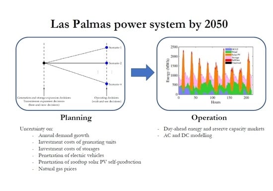
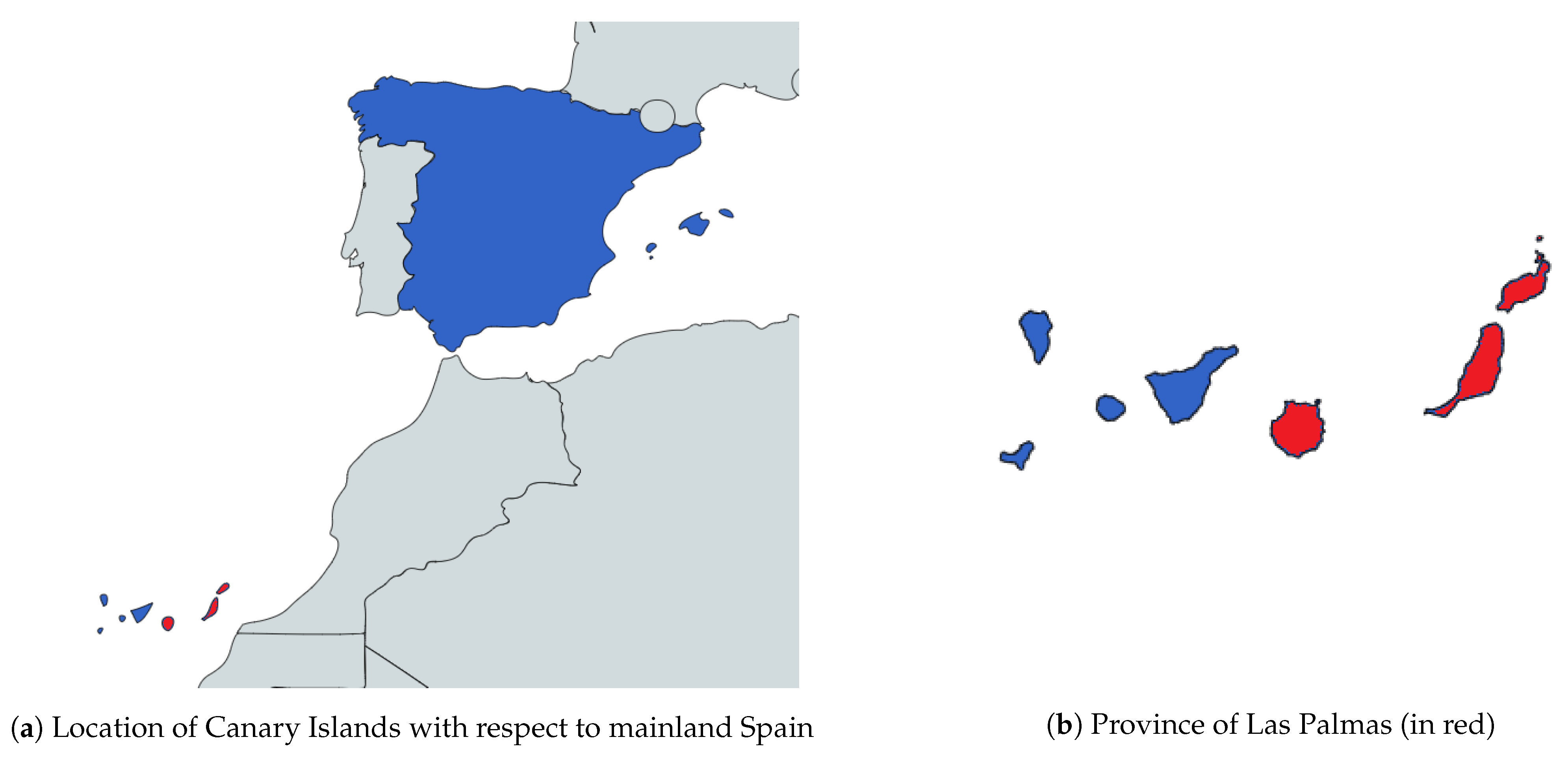
The objective of this paper is to design a renewable-dominated isolated power system of Las Palmas, Spain, by the year 2050. Las Palmas belongs to the Canary Islands archipelago and is one of the 50 provinces in which Spain is divided into. Figure 1 represents graphically the location of the Canarian Islands and Las Palmas. Las Palmas comprises 3 main islands: Gran Canaria (GC), Lanzarote (LZ) and Fuerteventura (FV). Figure 1b represents in red color those islands belonging to Las Palmas and in blue color the rest of Spain. The power systems of Lanzarote and Fuerteventura are linked since 2015 by a submarine AC cable of 132 kV with a rated capacity of 120 MVA pursuing the objective of increasing the strength of the grid and improving the capacity of integration of new renewable generation [3].

In order to determine the most convenient power system configuration of Las Palmas from technical and economical points of view, a two-stage Generation, Storage and Transmission Expansion Problem (GSTEP) is formulated. The uncertainties considered in this model are the investment costs of immature generating and storage technologies, the annual demand, the number of electric vehicles, the rooftop solar photovoltaic (PV) capacity penetration and natural gas prices. The operation of the resulting power system is modelled considering the energy and reserve capacity markets. Therefore, the main objective of this paper is to determine the investment decisions in generating, storage and transmission capacities to be made in the next years to minimize the total cost, including investment and operation costs. To that end, different minimum renewable energy output requirements can be enforced to ensure the achievement of a renewable-dominated system.

Many works have been devoted to analyze the integration of renewable energies in the Canary Islands. For instance, reference [4] analyzed the results obtained after the application of the first wind power development plan in the Canary Islands. This work concludes that the percentage of wind power capacity installed in the Canary Islands at the end of the planning horizon was smaller than that in mainland Spain, but higher than in most European countries. Reference [5] assesses the socio-economic potential of wind power in Gran Canaria and Tenerife. Reference [6] proposes a dynamic model to analyze the installation of a pumped-hydro storage system on Gran Canaria to increase the level of wind power penetration. Reference [7] determines the optimal size of a hydro pumping unit powered by wind in the island of El Hierro. The authors of [8] develop a cross-sectoral procedure considering electricity, heating, cooling, desalination, transport and gas sectors to take advantage of possible synergies to obtain a renewable-dominated system in Gran Canaria. Reference [9] proposes a procedure to achieve by 2050 a 100% renewable power supply for the entire archipelago considering power links between islands. The generation expansion problem in the isolated power system of Lanzarote-Fuertenventura has been formulated in [10,11] considering (i) the active participation of electric vehicles and (ii) reserve provision by wind power units, respectively. The potential of on-roof solar PV in the Canary Islands has been discussed in [12]. The potential of biomass in the Canary Islands has been assessed in [13]. The influence of natural gas in the future power system of the Canary Islands has been investigated in [14,15]. Planning and operating different isolated power systems have been studied in recent years. For instance, reference [16] proposes a novel control-system to increase the renewable penetration that has been tested on the King island power system. This approach is able to obtain fuel savings with respect to conventional control schemes. The authors of [17] have developed a multiyear expansion-planning optimization model for the Azores archipelago. The obtained results indicate that the interconnection among different isolated systems increases the usage of clean energies. Reference [18] has proposed a stochastic planning model devoted to the determination of the renewable transition in isolated Artic power systems. This work concludes that an adequate representation of the variability of renewable sources is key to obtain a robust power system configuration. Finally, reference [19] studies the Tilos island power system in Greece and analyzes the actual implementation of a configuration based on renewable energies and storage systems.

The technical literature concerning GSTEP approaches is large, [20]. The work developed in [21] solves this problem considering the demand, and the availability of generating units as uncertain parameters. Reference [22] also presents a generation and transmission expansion problem formulation but considering uncertain failures of generating units and transmission lines. The authors of [23] use equilibrium constraints to formulate the transmission expansion problem considering investments in wind power. Reference [24] formulates the generation and transmission expansion problem using a three-level equilibrium model. The transformation process of a thermal-dominated system into a renewable-dominated one is formulated in [25]. Reference [26] develops a stochastic adaptive robust optimization approach considering simultaneously long- and short-term uncertainties. The authors of [27] also propose a three-level adaptive robust optimization problem to model this problem. A multistage approach is developed in [28] to determine generation, storage and transmission investments. Reference [29] accounts for the spatial distribution of wind speed on the generation and transmission decisions. In [30], GSTEP is formulated considering a precise modeling of the technical constraints of generating units. Reference [31] proposes a mixed-integer linear formulation for the GSTEP placing also emphases in the mathematical modeling of the technical aspects of generating units. Finally, the authors of [32] compare the outcomes of different generation expansion models under uncertainty considering different number of decision stages.

The main contributions of this paper are twofold:

• To design a novel procedure for determining the generation, storage and transmission expansion of a realistic power system. The input data of Las Palmas power system have been elaborated in depth by the authors using publicly available sources, research works and technical reports.
• The uncertainty associated with investment costs of immature generating and storage technologies, the annual demand growth, the number of electric vehicles, rooftop solar photovoltaic capacity penetration and natural gas prices has been explicitly considered in this paper. To the best of the authors’ knowledge this is the first work that analyzes this set of uncertain parameters in the GSTEP.

Other specific contributions of this paper are the following:

• The rooftop solar photovoltaic potential in Las Palmas power system has been estimated in detail considering each municipality separately.
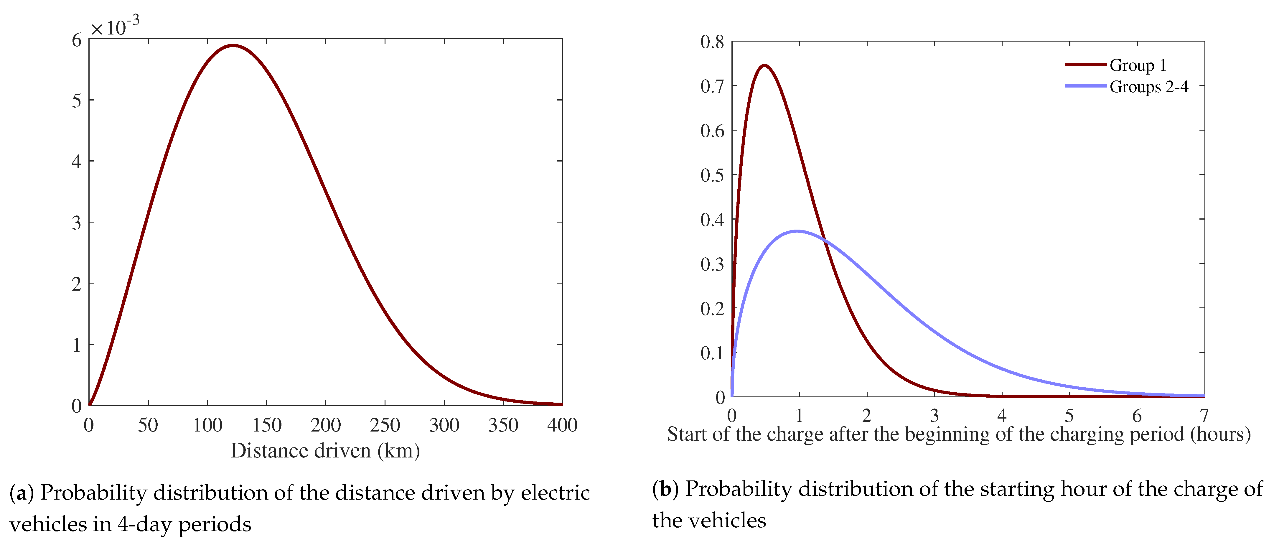
• A novel procedure for estimating the charging profiles of electric vehicles has been proposed using parametric distributions for characterizing the distance driven and the starting charge hour of electric vehicles.
• Two novel mixed-integer linear programming formulations have been proposed to determine the system-adequacy and reserve-capacity requirements of a power system formed by several isolated systems.
• The reserve-capacity participation of storages has been modeled considering simultaneously the maximum and minimum possible levels of energy stored in each time period depending on the deployment of the scheduled reserves and the participation in the day-ahead energy market.
• Unlike usual capacity expansion analyses, this paper includes the elaboration of an out-of-sample analysis to test the performance of the resulting power system during a whole year considering the AC modeling of the system.

The paper is structured as follows. The input data used to define the numerical study is described in Section 2. The methodology proposed to formulate the planning model is described in Section 3. The uncertainty characterization is provided in Section 4. The resulting generation, storage and transmission expansion decisions are provided and discussed in Section 5. The influence of the uncertain parameters and the renewable energy potentials in the expansion plans are analyzed in Section 6. Finally, the main conclusions of this study are drawn in Section 7. In the Appendix A, the mathematical formulation of the proposed GSTEP is included and described.

2. Characterization of Las Palmas Power System

The system considered in the study is formed by the transmission network, generation units and loads installed in the Spanish province of Las Palmas, comprising Gran Canaria, Lanzarote and Fuerteventura. This system comprises two isolated power systems: Gran Canaria (GC) and Lanzarote-Fuerteventura (LZ-FV). The topology of both power systems is depicted in Figure 2, where existing and candidates lines are represented. Observe that some candidate lines are planned over existing corridors, whereas other candidate lines are expected to create new corridors. Green lines are used to denote the HVDC cable that can be installed to link together both isolated systems. More details about the description of this system are provided below.

2.1. Potential Generating Capacity

The candidate thermal units considered in this study are open-cycle gas turbines (OCGTs). OCGTs burn natural gas to rotate a turbine using the combustion gases. A compressor forces the injection of air in the chamber for increasing the efficiency of the generating unit. OCGTs are scalable for different electric power capacities (typically from 10 to 600 MW) and they are suitable to be used for peak load electricity production. They emit 510 gCO${}_2$/kWh in average [33]. The selection of OCGT as candidate generation technology in Las Palmas power system has been made by three reasons: (i) the natural gas sector is of great importance in Spain (the leading Liquefied Natural Gas (LNG) importer in the European Union in 2020 [34]) and this sector is expected to play a role in future Spanish systems, (ii) the existence of small-sized OCGTs specially tailored for isolated power systems and (iii) the high flexibility of these units, which are characterized by high ramping capabilities and short startup times. These characteristics make them appropriate to be installed in isolated power systems with high presence of intermittent units.

The operation cost of OCGTs is obtained from [35], that describes the operation costs for different electricity generation technologies in isolated power systems in Spain. The thermal consumption of OCGTs is linearly expressed as a function of the electric power produced and is equal to 4.457 MW-t/MW. The fixed operation and management cost per unit is 9.25 €/MWh.

Additionally to OCGTs, it is considered that wind and utility-scale PV power units can be installed. It is assumed that the installation of rooftop solar PV facilities is not decided by the system planner. In this manner, the future capacity of this type of facilities is modeled as an uncertain parameter.

The capital costs of generating units are included in

Table 1. Capital costs of generating and storage units.

Technology	Capital Cost
	(€/kW)
OCGT	660
Wind	1452
Solar PV	660

. The capital costs of generating units are obtained from [33] and they are increased 10% because of the geographical situation of Las Palmas. The candidate generating units to install are provided in

Table 2. Technical characteristics of candidate generating units.

Techn.	Unit	Node	Potential Capacity (MW)	Techn.	Unit	Node	Potential Capacity (MW)
OCGT	1–10	26	32.0	Solar PV	66	5	7.6
	11–20	26	32.0		67	8	18.6
	21–32	26	32.0		68	6	153.0
	33–44	26	32.0		69	7	29.4
Wind	45	3	50.3		70	9	22.3
	46	2	12.3		71	10	6.0
	47	2	193.4		72	11	38.4
	48	5	196.0		73	12	23.2
	49	8	654.8		74	13	23.2
	50	6	61.2		75	14	23.2
	51	9	22.8		76	15	23.2
	52	22	165.8		77	16	23.2
	53	23	2.4		78	17	23.2
	54	24	1.8		79	18	23.2
	55	26	111.1		80	19	23.2
	56	31	143.6		81	20	23.2
	57	37	0.6		82	22	235.6
Solar PV	58	3	166.4		83	23	190.2
	59	1	0.4		84	24	302.9
	60	2	61.9		85	26	12.0
	61	2	1.5		86	31	50.8
	62	3	22.9		87	35	8.7
	63	3	4.0		88	36	18.5
	64	4	33.5		89	37	5.4
	65	7	29.9

. It is assumed that the total capacity of each OCGT unit must be installed if the unit is selected to be built. On the contrary, given the modularity characteristics of wind and solar PV technologies, it is considered that the power in the installed candidate units belonging to these technologies can comprise between zero and the potential capacity of each candidate unit.

2.2. Storage Capacity

We consider that utility-scale storage units based on Li-ion batteries can be installed to increase the operation flexibility of the system. Li-ion batteries are suitable to be used in power grid applications, including load shifting [2]. In this sense, Li-ion batteries outperform competing technologies as Ni–metal hybrid, Ni-Cd, and Pb–acid in terms of delivered energy while providing high specific power. Additionally, Li-ion batteries present a higher efficiency (90–94%) than Na-S batteries (70%) and a similar number of cycles (4500). Furthermore, Li-ion batteries are experimenting a significant impulse because of the reduction of their capital costs motivated by the research efforts related to the electric vehicle industry.

The location and size of storages are co-optimized in the proposed GSTEP. In this manner, storage facilities can be installed anywhere from a set of available locations. For instance, in this case study it has been decided that new storages can be installed in those buses where thermal units are currently at operation. These buses have been selected as available locations because they have adequate transmission facility infrastructures allowing a proper evacuation of the energy stored in these facilities. The sizes of the installed storages, in terms of power and energy capacities that can be installed in an available storage location are mathematically modeled as continuous variables. We refer the reader to the Appendix A for further information on the mathematical formulation of storages. A typical relationship between power and energy terms equal to 6 h is considered. The location of the candidate storage units and the maximum storage capacity, in power and energy units, is listed in

Table 3. Technical characteristics of candidate storage units.

Unit	Node	Potential Capacity (MW)/(MWh)
1	1	300/1800
2	2	300/1800
3	6	300/1800
4	8	300/1800
5	21	300/1800
6	22	300/1800
7	26	300/1800
8	31	300/1800

.

2.3. Transmission Network

The data associated with the transmission network under study is owned by Red Eléctrica de España, who is the Spanish Transport System Operator [3]. The authors contacted the operator asking for the data necessary to perform the type of studies presented in this work but unfortunately the data were not available. So, the topology and parameters considered for the study have been obtained from different publicly available sources like [36,37,38,39,40]. This information has been complemented with academic and research works such as [6,41].

The transmission network is operated in three different voltage levels: 66, 132 and 220 kV. The lines of 132 kV form the backbone of the system but new lines of 220 kV have been installed in recent years to take this role. That investment in new lines has been realized in order to improve the power quality and facilitates the installation of more renewable generation based on wind energy and solar PV. Transmission lines have been represented using $\pi$ model and the conductance is neglected. The principal characteristics of the lines considered in this work are presented in

Table 4. Principal characteristics of existing transmission lines considered in the study.

Conductor ${}^1$	Voltage (kV)	Area ${}^2$ (mm${}^2$)	Diameter ${}^3$ (mm)	Resistance (Ω/km)	Reactance (Ω/km)
${}^o$ LARL-125 (Penguin)	66	125.1	14.31	0.2846	0.3976
${}^o$ LARL-280 (Hawk)	66	281.1	21.78	0.1276	0.3712
${}^o$ LARL-380 (Gull)	66	381.0	25.38	0.0930	0.3616
${}^o$ LARL-380 (Gull)	132	381.0	25.38	0.0931	0.4057
${}^o$ LARL-516 (Rail)	220	516.8	29.61	0.0681	0.4015
${}^u$ 300 Cu	66	300	51	0.1379	0.0588
${}^u$ 400 Cu	66	400	54	0.1456	0.0661
${}^u$ 630 Cu	66	630	62	0.1280	0.0609
${}^u$ 630 Al	66	630	62	0.1466	0.0613
${}^u$ 800 Al	66	800	66	0.1379	0.0588
${}^u$ 1000 Al	66	1000	70	0.1307	0.0560

${}^1$: nomenclature from [43]; ${}^2$ Conductor area; ${}^3$ Outer diameter of cable; ${}^o$: overhead; ${}^u$: underground.

and have been obtained from [36,41,42,43]. The electrical parameters in Table 4 are referred to the positive sequence value, a nominal frequency of 50 Hz and a temperature of the cable of 50 ºC. For the case of underground lines it is assumed that are formed by cross-linked polyethylene (XLPE) insulated cables and are placed 1.5 m under the surface. The transposition of the lines have not been considered due to the relative small length of the lines. In fact the transposition arrangement is necessary if the three-phase AC line is more than 100 km, but in the power system under study no AC line is more than 26 km long so the assumption is correct. The total length of transmission lines between 66 and 220 kV in the considered representation of Las Palmas power systems is 704 km.

The characteristics of candidate lines are provided in

Table 5. Characteristics of candidate lines (LARL-380 (Gull)).

Capacity (MW)	Voltage (kV)	Resistance (Ω/km)	Reactance (Ω/km)	Existing Corridor	Cost (k€/km)
80	66	0.0930	0.3616	No	373
				Yes	264
160	66	0.0465	0.1808	No	621
				Yes	439
240	66	0.0310	0.1205	No	812
				Yes	703

. All candidate lines are 66 kV overhead transmission lines to be placed in either existing or new corridors. The values presented in this table are based on [44] where it is publicly exposed the request from the transmission system planner to the Regional Government of Canarias for administrative authorization of the construction of a transmission line.

Table 6. Candidate lines.

Line	Origin Bus	Destination Bus	Length (km)	Voltage (kV)	Capacity (MW)
1	1	2	8.9	66	80
2	1	3	25.0	66	80
3	9	10	9.0	66	160
4	9	37	17.0	66	160
5	11	12	10.0	66	160
6	12	13	9.0	66	160
7	12	15	4.0	66	160
8	14	19	2.0	66	80
9	14	21	7.7	66	80
10	14	21	7.7	66	160
11	14	21	7.7	66	240
12	15	16	2.0	66	80
13	18	19	2.0	66	160
14	18	19	2.0	66	240
15	21	24	8.1	66	80
16	21	24	8.1	66	160
17	22	23	8.0	66	80
18	23	24	9.0	66	80
19	23	24	9.0	66	160
20	26	27	0.7	66	80
21	27	31	15.0	66	80
22	28	22	6.0	66	80
23	28	31	15.0	66	80
24	31	33	9.6	66	80
25	33	36	12.0	66	80
26	36	37	20.0	66	80
27	26	7	160.0	132	100

provides the specifications of candidate lines. Observe that only two candidate lines, 1–2, are proposed for LZ-FV power system, whereas candidate lines 3–26 are placed in GC system. The reason for this is that LZ-FV system is simpler than GC system and it is also better suited to accommodate a large capacity of new generating units. Finally, line 27 is the transmission link between both systems formed by a 160 km long DC submarine cable, with a capacity of 100 MW and an expected investment cost of 474.5 M€, [36]. Candidate lines, together with existing lines, are depicted in Figure 2.

2.4. Temporal Representation

A set of characteristic days is used to represent the target year. For each day, the hourly values of renewable availability and system demand are considered to characterize the temporal variability of these parameters. The specific days used to represent the year have been selected using the fast-forward algorithm proposed in [45]. In this manner, the fast-forward algorithm is implemented taking as input data the net demand of Las Palmas power system in year 2018 for each day and hour, which is computed as the total demand minus the renewable production. As a result, 9 characteristic days (216 hourly periods) are selected to represent the target year.

Table 7. Selection of characteristic days.

Selected Days	Selection Order	Weight	Normalized Demand (pu)	Normalized Wind Availability (pu)	Normalized Solar PV Availability (pu)
14 January 2018	6	15	1.005	1.105	0.353
16 January 2018	7	15	1.055	2.143	0.501
16 March 2018	1	199	1.012	1.046	1.007
6 May 2018	3	13	1.128	0.110	0.711
13 May 2018	2	13	0.859	2.418	0.859
14 May 2018	9	42	0.944	2.177	1.465
24 June 2018	8	18	0.895	0.342	1.410
13 July 2018	5	30	0.962	0.109	1.042
25 October 2018	4	20	0.930	0.238	0.262

provides the main information about the selection process of characteristic days. The selection order of each day, the weight and the normalized daily demand and wind and solar PV availabilities are included in this table. Values are normalized by the average daily values. Note that the day with highest weight, 16 March 2018, was selected in the first position and it has normalized values of demand and wind and solar PV availabilities close to 1.

The hourly availability of the renewable power production for each characteristic day in each island is provided in Figure 3.

Figure 4 represents the hourly demand for each characteristic day in each island. Observe that the demand in GC is significantly higher than that in the rest of islands (almost four times higher).

3. Methodology

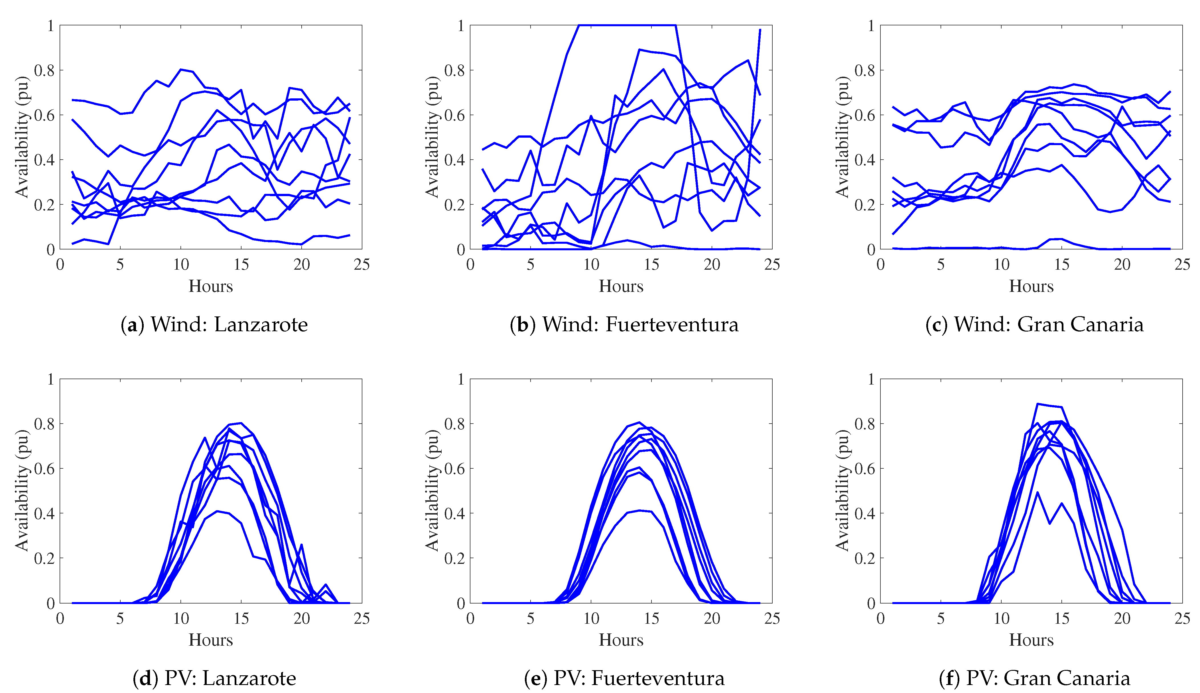
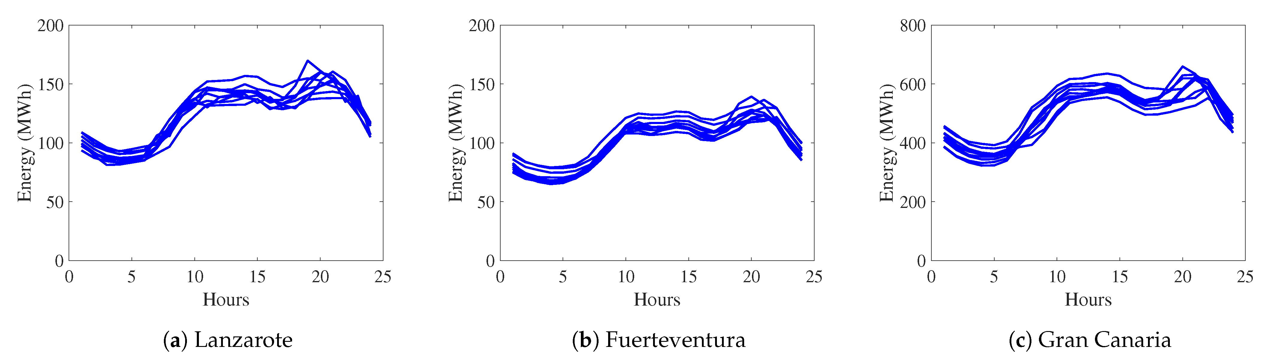
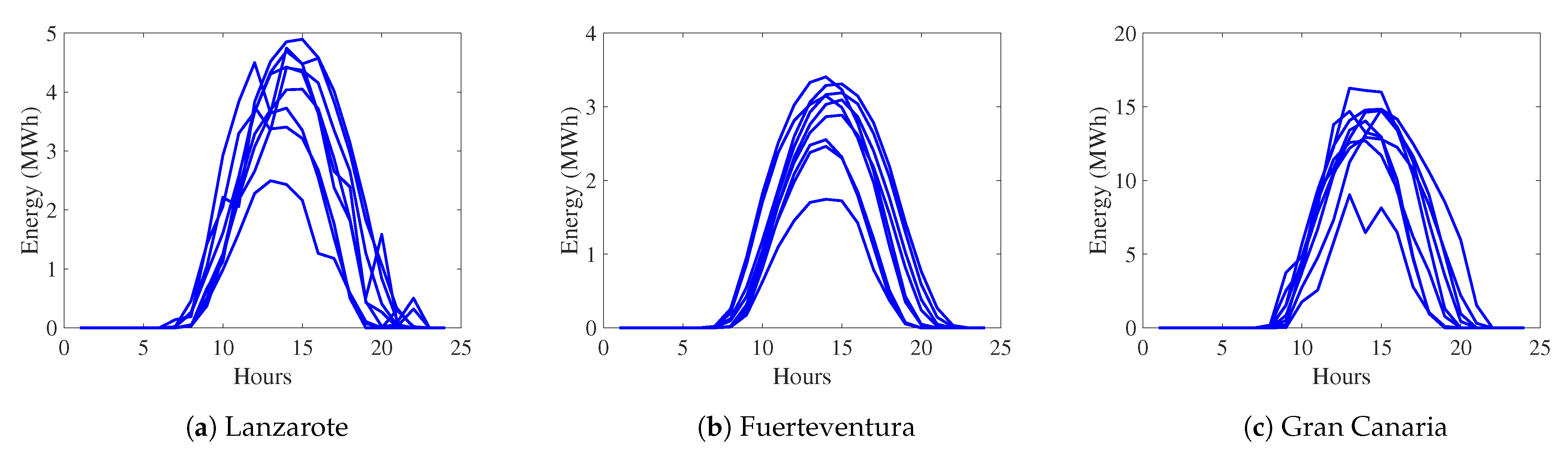
The methodology used to determine the generation, storage and transmission capacity decisions in Las Palmas power system is described in this section. A set of candidate generating and storage units is defined for each bus of the system. Additionally, a set of candidate transmission lines is considered for each island. The description of the candidate investment assets is provided below. The investment decisions to determine consist in: (i) the power capacity to be installed from the candidate set of generating units, (ii) the power/energy capacity to be installed from the set of candidate storage units and (iii) the transmission lines to be installed from the set of candidate transmission lines. Investments on new assets are considered to be at operation in 2050. The variability of the intermittent power production, demand, charge of electric vehicles and rooftop solar PV self-production is characterized in an hourly basis, as indicated in Section 2. The proposed mathematical formulation and its notation are described in detail in the Appendix A.

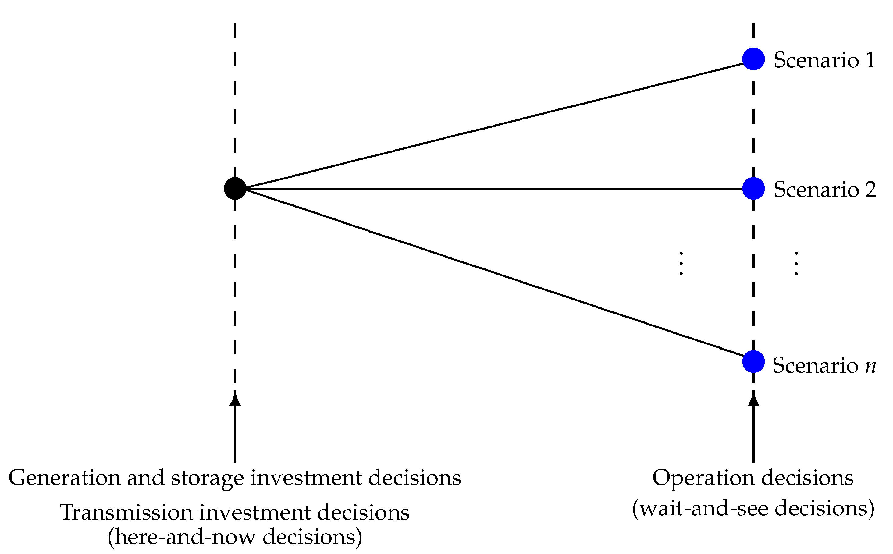
Note that different uncertainties affect to the investment decisions to make in the planning of a power system. In order to handle this uncertainty, a stochastic programming model is proposed. Figure 5 represents graphically the decision-making framework adopted in this work. The black point represents the time in which investment decisions are made. These are here-and-now decisions that are made before knowing the actual realizations of the uncertain parameters. The operation of the resulting power system is simulated in the second stage after knowing the realizations of the uncertain parameters. For this reason, operation decisions represented by blue circles are considered as wait-and-see decisions, which can be different for each scenario. The power system operation consists of the scheduling of the day-ahead energy and reserve capacity markets.

As it is usual in capacity expansion models, investment costs are annualized using the capital recovery factor (CRF), where CRF $=\frac{r{(1+r)}^x}{{(1+r)}^{x-1}}$, x is the expected life of the asset, and r the interest rate. In this study, the expected life of assets is 25 years and the interest rate is 9%. The operation costs of the resulting power system are simulated in the investment capacity problem by modeling the scheduling of the day-ahead market, considering simultaneously energy and up/down reserve capacity markets. These markets are settled down using the estimated values of the demand and wind and solar PV productions. These values are generated by using historical data from 2018 available in [46]. The transmission network is accounted for in the day-ahead market scheduling and it is represented using a DC model. Storages are assumed to store 0.5 times their energy capacities at the beginning of each day, and they have to be also charged up to that value at the end of the day. The operating costs of intermittent and storage units are assumed to be negligible. The unserved demand penalization cost is equal to 1000 €/MWh. The up and down reserve capacity requirements of the system are computed using the procedure described in [47]. In this manner, up and down reserve capacities must be greater than 3% of the demand plus 5% of the intermittent production in each hour. Reserve capacity costs are equal to 0.25 times the operating cost for each unit. It is assumed that wind and solar PV units are not qualified to supply reserve capacity.

Finally, the power system adequacy has been explicitly formulated in the proposed model. This adequacy refers to the ability of the power system to supply its peak load through electricity generation under normal operating conditions. Therefore, the total installed capacity considering all technologies has to be greater than the highest expected demand. In order to ensure power system adequacy, the power capacities of OCGT and storage units have been derated 10%. Considering that the peak demand happens at night in this system and the non-dispatchability of intermittent power units, wind and solar PV capacities have been derated 90 and 100%, respectively. The peak demand is equal to 1.2 times the maximum hourly demand expected in 2050 in each system. The provision of frequency support is not modeled in this work. It is assumed that inverter-connected generation and storage units will be able to support system inertia in 2050 by the provision of virtual inertia. The provision of virtual inertia has been investigated in [48,49,50,51].

4. Uncertainty Modelling

In the proposed procedure, future investment costs of immature generating and storage technologies, the annual demand growth, the self-production penetration, the number of electric vehicles and natural gas prices are explicitly considered as uncertain parameters. The possible values of these uncertain parameters are modeled by a set of scenarios. Therefore, each scenario is a plausible realization of the uncertain parameters. These scenarios are generated based on the predictions made by energy agencies. This scenario-generation procedure is applied if there exist insufficient data or knowledge about the future [52]. Considering that this paper aims at solving a large-scale long-term decision making problem to determine the generation, storage and transmission capacities, the short-term operation uncertainties as generation unit failures or degradation of storage units have been disregarded to reduce the computational complexity of the resulting optimization problem. The description of the modelling of each considered uncertain parameter is explained below.

4.1. Investment Costs of Immature Generation Technologies and Storages

Considering that the different generation, storage and transmission assets should be at operation by the year 2050, all investment costs are estimated for year 2040. The investment costs of renewable technologies are based on the estimations provided by IEA [53]. As indicated in Table 1, capital costs of wind and solar PV power units are equal to 1452 and 660 €/kW. Three scenarios are generated considering that possible investment costs can be either equal to the expected ones, 10% higher or 10% lower. Similarly, the investment costs of storage units are modeled using three scenarios which are equal to 80, 148 and 212 €/kWh, as estimated in [54] for 6-h Li-on batteries.

4.2. Demand

The electrification, or substitution of electricity for direct combustion of non-electricity-based fuels, is the main cause motivating the highly increase of electricity demand in the incoming years. In fact, IRENA indicates in [55] that the share of electricity in total energy consumption will move from 20% in year 2018 to 49% in 2050 if a 70% reduction on CO${}_2$ emissions is required. The increase of electricity demand will come mainly from the heating and transportation sectors. According to [56], 3 electricity demand scenarios, without considering the electricity demanded by electric vehicles, are computed by scaling up the electricity demand in each island in 20, 25 and 30% with respect to the values observed in 2018. The demand associated with the charge of electric vehicles will be modeled below considering different penetrations of electric vehicles.

4.3. Rooftop Solar PV Self-Production Penetration

The self-production capacity of solar PV rooftop facilities connected to each bus can be estimated using different procedures. For instance, the procedure described in [57] considers the population density of the cities associated to each bus, whereas [58] takes also into account the building density to estimate the roof available area that can be dedicated to rooftop facilities. Assuming the conservative criteria that each installed kW requires a space of 7 m${}^2$ [59], the procedures described in [57,58] estimate maximum capacities equal to 2338 and 1818 MW, respectively.

Considering the most unfavorable situation, the capacity obtained from the procedure described in [58] is considered in this work. This procedure categorizes building and population-density per municipality as low (L), medium (M), high (H) and very high (VH). Next, according to the building- and population-density category assigned to each municipality, the available roof area per capita is computed. In general, the roof area per capita increases as the building and population-density reduces. For instance, in the Spanish case, a building- and population-density category denoted by L-L has associated 76.4 km${}^2$/capita, whereas the available roof area per capita in category VH-VH is equal to 6.7 km${}^2$/capita.

Table 8. Solar PV self-generation potential capacity estimation.

Island	Municipality	Population 2050	Popul. Density (inhab/km${}^2$)	Area (km${}^2$)	Building Density-Population Density	Self-Production Area (km${}^2$)	Occupied Area (%)	Self-Production Capacity (MW)
LZ	Arrecife	62,988	2651.01	23.76	L-H	1.321	5.56	188.7
	Haría	5123	45.58	112.40	L-L	0.107	0.10	15.3
	San Bartolomé	18,816	446.29	42.16	L-L	0.395	0.94	56.4
	Teguise	22,342	83.25	268.37	L-L	0.469	0.17	66.9
	Tías	2017	312.18	6.46	L-L	0.042	0.65	6.0
	Tinajo	6279	46.41	135.29	L-L	0.132	0.10	18.8
	Yaiza	16,571	78.22	211.85	L-L	0.347	0.16	49.6
FV	Antigua	12,461	45.52	273.75	L-L	0.261	0.10	37.3
	Betancuria	758	7.9	95.95	L-L	0.016	0.02	2.3
	La Oliva	2658	74.64	35.61	L-L	0.056	0.16	8.0
	Pájara	21,093	55	383.51	L-M	0.442	0.12	63.2
	Puerto del Rosario	40,753	140.55	289.95	L-M	0.855	0.29	122.1
	Tuineje	15,241	55.24	275.91	M-H	0.320	0.12	45.7
GC	Agaete	5586	125.47	44.52	VL-VL	0.117	0.26	16.7
	Agũimes	31,619	401.87	78.68	M-H	0.285	0.36	40.7
	La Aldea de S. Nicolás	7504	60.71	123.60	VH-VH	0.045	0.04	6.5
	Artenara	69	16.09	4.29	VL-VL	0.001	0.03	0.2
	Arucas	38,138	1165.94	32.71	M-VH	0.213	0.65	30.4
	Firgas	7455	465.36	16.02	VL-VL	0.156	0.98	22.3
	Gáldar	24,242	388.49	62.40	H-H	0.336	0.54	48.0
	Ingenio	31,321	801.87	39.06	M-H	0.282	0.72	40.3
	Mogán	2072	117.16	17.69	M-M	0.057	0.32	8.1
	Moya	7696	239.23	32.17	VL-VL	0.161	0.50	23.1
	Las Palmas de GC	379,925	3755.84	101.16	H-VH	2.564	2.54	366.4
	S. Bartolomé de Tirajana	5443	160.72	33.87	L-M	0.106	0.31	15.1
	Sta. Brígida	18,263	766.39	23.83	VL-VL	0.383	1.61	54.7
	Sta. Lucía de Tirajana	73,328	1173.62	62.48	VL-VL	1.538	2.46	219.7
	Sta. María de Guía de GC	13,850	330	41.97	VL-VL	0.290	0.69	41.5
	Tejeda	1909	18.38	103.86	VL-VL	0.040	0.04	5.7
	Telde	102,647	1023.6	100.28	H-VH	0.693	0.69	99.0
	Teror	12,519	485.23	25.80	VL-VL	0.263	1.02	37.5
	Valleseco	3749	169.48	22.12	VL-VL	0.079	0.36	11.2
	Valsequillo de GC	9340	240.72	38.80	VL-VL	0.196	0.50	28.0
	Vega de San Mateo	7556	197.75	38.21	VL-VL	0.158	0.41	22.6
TOTAL		1,011,331	474.87	3198.49	-	12.73	0.40	1817.9

provides the expected self-generation potential for each municipality. We refer the interested reader to [58] for additional information about this procedure.

Over the maximum potentials computed per bus, three conservative scenarios of 1, 5 and 10% penetration of self-production capacity are considered. The power production of self-production facilities is assumed to be equal to 0.8 times the per-unit available production generated by utility-scale solar PV units to take into account the lacks of efficiency caused by the non-optimal orientation and inclination of solar panels in rooftop facilities with respect to utility-scale plants. Figure 6 represents the rooftop solar PV production for each representative day.

4.4. Number of Electric Vehicles

The Energy Roadmap 2050 requires that at least 95% of light-duty vehicles would be electric powered by year 2050 [60]. Considering this projection, the penetration of electric vehicles in Las Palmas has been characterized using three scenarios with values equal to 55, 75 and 95% of total vehicles. The total number of vehicles has been computed considering that the number of vehicles per person is 0.54 vehicles/person according to [61], and that the population in Spain is expected to decrease in 2050 over 10% with respect to 2019 [62].

The energy demand of electric vehicles has been modeled for each bus and day considering that the average daily distance driven by each vehicle is 35 km and that the energy consumption and the battery capacity of vehicles are equal to 0.2 kWh/km and 80 kWh, respectively, [63]. For each bus and day, charging profiles for 100 vehicles are randomly generated. The energy charged in each period is afterwards scaled considering the actual number of vehicles in each bus. The energy demanded by electric vehicles has been modeled using an approach based on that presented in [64]. Using this procedure, the start of the charging period and the daily distance driven by each vehicle are randomly generated. For that, according to the driving patterns of vehicle users in Spain [65], 4 different groups, (1)–(4), of electric vehicle users are defined according to the period in which they charge their vehicles: (1) between 00:00 and 7:00 h of next day, (2) between 16:00 and 7:00 h of next day, (3) between 2:00 and 14:00 h of next day, and (4) between 3:00 and 19:00 h. The percentage of vehicles in each group are 45, 35, 15 and 5%, respectively. It is assumed that vehicles are charged in average every 4 days (after driving an average of $35\times 4=140$ km). The daily distance driven each day by each vehicle is modeled using a Weibull distribution with mean equal to 140 and scale and shape factors equal to 158.02 and 2.25. This distribution is represented in Figure 7a. Note that the probability of driven distances out of the usage range of vehicles, 0-400 km, is null using this distribution. The starting charge hour for each group in each bus for each day is also modeled using a Weibull distribution with scale and shape factors equal to 2 and 1.5 for vehicles belonging to groups 2–4 and, and 1 and 1.5 for those in group 1. Observe that the number of hours available for charging vehicles in group 1 is only 8, whereas the rest of groups have more than 15 h for charging their vehicles. The probability distributions of the start of the charge is depicted in Figure 7b.

As an example, Figure 8 represents the two-day aggregated charging profile of a set of 1000 electric vehicles. The charging profile represented in this figure is randomly generated from the distribution functions depicted in Figure 7. Observe that the peak demand is around 750 kW and happens at 2:00 in the two analyzed days. At that hour, a significant part of the vehicles belonging to groups (1) and (2) is charging. Considering that electric vehicles charge at 7.4 kW, around 100 vehicles are simultaneously charging at that hour.

Figure 9 represents the generated charging profiles for each characteristic day in each island.

4.5. Natural Gas Prices

Natural gas price scenarios are obtained from [66]. The maximum and minimum prices are equal to 62.63 and 57.48 €/MWh-t and they constitute the maximum and minimum natural gas price forecasts for Spain in 2050 estimated by the International Energy Agency (IEA) considering current energy policies. Note that MW-t and MWh-t refer to thermal power and energy units, whereas MW and MWh denote electric power and energy units.

4.6. Scenario Description

Following the description of the uncertain parameters provided above,

Table 9. Parameters modeled through scenarios (per unit).

Parameters (%)	Low (L)		Medium (M)		High (H)
	Value	Prob.	Value	Prob.	Value	Prob.
(1) Capital cost of storages	0.54	$1/3$	1.00	$1/3$	1.43	$1/3$
(2) Capital cost of renewable units	0.90	$1/3$	1.00	$1/3$	1.10	$1/3$
(3) Demand in 2050	1.20	$1/3$	1.25	$1/3$	1.30	$1/3$
(4) Penetration of self production	0.01	$1/3$	0.05	$1/3$	0.10	$1/3$
(5) Penetration of electric vehicles	0.55	$1/3$	0.75	$1/3$	0.95	$1/3$
(6) Natural gas prices	0.46	$1/3$	1.00	$1/3$	1.43	$1/3$

contains in a compact-manner the considered scenarios for each uncertain parameter. As observed in this table, three equiprobable scenarios are considered for each parameter.

Considering that three possible values are defined for each of the 6 uncertain parameters described above, $3^6=729$ scenarios are generated. The cardinality of this set of scenarios has been reduced up to 7 by using the scenario reduction technique described in [67].

The resulting scenarios are included in

Table 10. Selected scenarios.

Scenario	Parameters						Probability
	(1)	(2)	(3)	(4)	(5)	(6)
1	0.54	1.10	1.25	0.10	0.95	0.46	0.2551
2	1.43	1.10	1.30	0.05	0.55	1.43	0.0069
3	1.00	1.10	1.25	0.01	0.75	1.43	0.0974
4	0.54	0.90	1.20	0.10	0.55	0.46	0.0645
5	1.00	1.10	1.25	0.01	0.55	1.00	0.2565
6	1.43	0.90	1.25	0.05	0.55	1.43	0.0261
7	1.43	1.10	1.30	0.05	0.95	0.46	0.2936

. Note that each parameter is denoted by the number indicated in Table 9.

Observe that the considered demand profiles, including the energy charged by electric vehicles, may be subjected to modifications in planning models if demand-side management actions are implemented [68]. Examples of demand-side management may be load shifting or interruptible load services. However, we have not found sound estimations about the expected implementation of this type of services in the considered system for 2050. For this reason, we have assumed a conservative position from the planner point of view, and demand-side management actions are not considered in this GSTEP.

5. Results and Discussion

In this section, we include the results obtained by solving the generation, storage and transmission expansion model described above. All mathematical problems have been solved using GAMS (see [69]) and CPLEX 12.6.111 (see [70]) in a linux-based server of four 3.0 GHz processors and 250 GB of RAM. Regarding the computational cost, each single case has been solved in less than 36 h.

A number of cases have been solved to test the performance of the proposed procedure and to quantify, qualitatively and quantitatively, the influence of the variation of some key parameters in the resulting generation, storage and transmission expansion. First, a base case has been solved considering the input data described in Section 2. This solution is compared with that obtained if a minimum percentages of non-thermal power production is enforced (95%). Additionally, the base case solution has been compared with that obtained if the transmission link between the power systems of GC and LZ-FV is built. Finally, an out-of-sample analysis has been performed using the demand and renewable power availability observed in year 2019. For doing that, an optimal power flow has been solved for each hour of the year considering the AC modeling of the power system.

5.1. Results from the Investment Model

This section analyzes the following three cases:

• Base. This case corresponds with solving the generation, storage and transmission expansion problem considering the input data described in Section 2.
• 95%Ren. This case is similar to Base case but enforcing that at least 95% of the power production must be generated from non-thermal generating units.
• FixedLink. This case is similar to Base case but enforcing that the transmission link between the power systems of Gran Canaria and Lanzarote-Fuerteventura is built.

Table 11. Annualized expected costs (million €).

Case	Generation Investment	Storage Investment	Transmission Investment	Day-Ahead Energy	Reserve Capacity	Unserved	Total Demand
Base	428.6	142.0	4.53	188.6	45.9	0.00	809.6
95%Ren	713.0	171.3	7.08	67.6	50.3	136.18	1145.4
FixedLink	429.8	129.9	55.79	197.3	45.2	0.00	858.0

provides the expected costs resulting in each case. This table reveals that, for every case, the investments in new generation units achieve the highest costs. On the contrary, investments in transmission lines are much lower, specially in Base and 95%Ren cases. If Base and 95%Ren cases are compared, it can be concluded that imposing a strong minimum requirement of non-thermal production (at least 95%) leads to higher generation, storage and transmission investment costs. Particularly, the investments costs in these three concepts in 95%Ren case are 66.4, 20.6 and 56.3% higher than those in Base case, respectively. However, the day-ahead energy costs decrease 64% in 95%Ren case because of the low operation costs of renewable units. The increased usage of renewable units has the non desirable consequence of increasing the reserve capacity costs, which grow in 95%Ren case 9.6% with respect to those in Base case. It is worth noting that there is unserved demand in 95%Ren case, which is equal to 1.42% of the total demand.

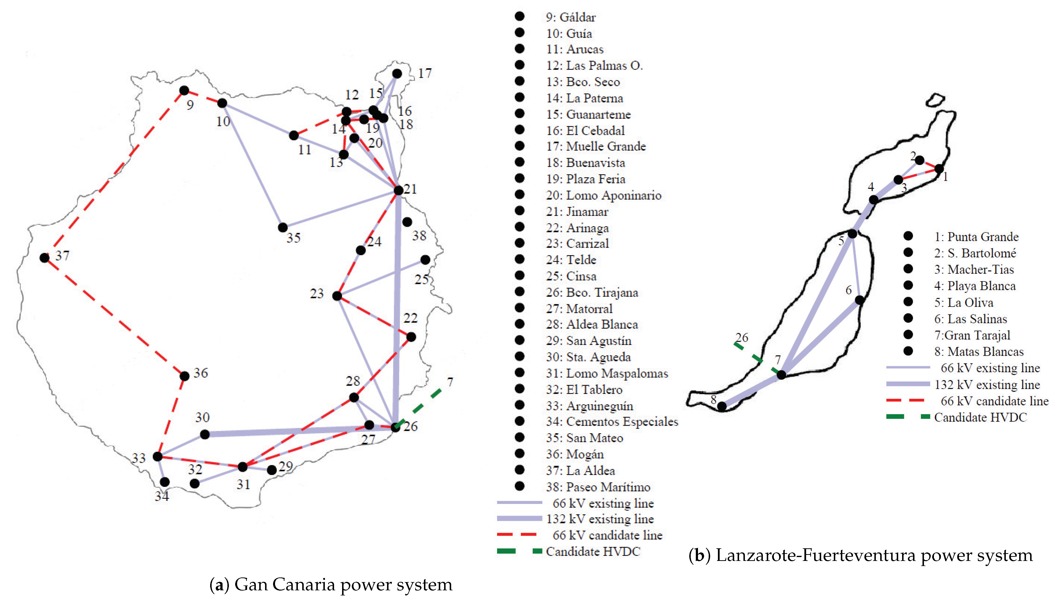
If the impact of building a power line between GC and LZ-FV power systems on total costs is analyzed, it can be observed that the total cost increases 6%. Therefore, we can conclude that linking GC and LZ-FV power systems cannot be only justified by economic reasons. Additionally, other factors as security supply or efficiency must be taken into account in order to analyze the installation of this transmission facility. The most relevant consequence of installing the linking line between both systems is that the total investment cost of storage units decreases significantly, 8.5%.

Table 12. Generation and storage capacity to be installed (MW).

Case	Island	OCGT	Wind	Solar PV	Storage
Base	LZ	64.0 (16.7%)	195.3 (38.2%)	556.4 (95.8%)	210.5 (35.1%)
	FV	64.0 (16.7%)	60.3 (3.3%)	461.8 (96.8%)	277.3 (46.2%)
	GC	352.0 (55.0%)	856.0 (95.5%)	1987.9 (90.2%)	1088.1 (90.7%)
	Total	480.0 (34.1%)	1111.7 (34.4%)	3006.1 (92.1%)	1575.9 (65.7%)
95%Ren	LZ	64.0 (16.7%)	512.0 (100.0%)	581.0 (100.0%)	326.9 (54.5%)
	FV	0.0 (0.0%)	1432.1 (78.5%)	477.0 (100.0%)	374.5 (62.4%)
	GC	256.0 (40.0%)	896.0 (100.0%)	2205.0 (100.0%)	1200.0 (100.0%)
	Total	320.0 (22.7%)	2840.1 (87.9%)	3263.0 (100.0%)	1901.5 (79.2%)
FixedLink	LZ	64.0 (16.7%)	219.7 (42.9%)	511.5 (88.0%)	214.9 (35.8%)
	FV	64.0 (16.7%)	74.3 (4.1%)	461.8 (96.8%)	150.9 (25.2%)
	GC	352.0 (55.0%)	878.4 (98.0%)	1915.6 (86.9%)	1076.5 (89.7%)
	Total	480.0 (34.1%)	1172.5 (36.3%)	2888.9 (88.5%)	1442.3 (60.1%)

lists the generation and storage capacity installed in each case. The percentage values in this table indicate the percentage of capacity installed over the potential of each technology in each island. It can be observed from the Base case that the generation technology most installed with respect to its potential is solar PV (92.1%). Opposite to this, OCGT and wind units are installed below 35% of their potentials. However, the wind power capacity installed in GC is 95%. The reason of this result is that this island has associated a much higher demand than the other two islands. It also interesting to note that the storage capacity installed in GC is above 90%, whereas it is below 50% in LZ and FV. The high penetration of intermittent power units in GC (above 90% in wind and solar PV units) motivates the high capacity of storage units installed in this island.

The generation and storage capacities installed in 95%Ren case are substantially different to those resulting in Base case. First, it is observed that the OCGT capacity is reduced 33%. As a consequence of this, the total capacity of renewable units (wind and solar PV) increases 39.7%, from 4597.8 to 6423.1 MW. This increase is mainly due to wind power, that grows from 1111.7 to 2840.1 MW (155.5%). In the same manner, the storage capacity increases 20.5%.

From the FixedLink case it can be noticed that the generation capacity installed is quite similar to that resulting from the Base case. However, a small reduction of solar PV capacity is observed, which is compensated by an increase of wind power units. As commented above, the storage investments in this case are significantly smaller than those in the Base case.

Table 13. Investments in transmission lines.

Case	Island	# Lines	Length (km)	Cost (k€)
Base	LZ	0	0.00	0.00
	FV	0	0 0.00	0.00
	GC	13	111.60	4532.45
	Link	0	0.00	0.00
	Total	13	111.60	4532.45
95%Ren	LZ	1	25.00	949.34
	FV	0	0.00	0.00
	GC	16	138.20	6127.42
	Link	0	0.00	0.00
	Total	17	163.20	7076.77
FixedLink	LZ	0	0 0.00	0.00
	FV	0	0 0.00	0.00
	GC	19	170.30	7479.68
	Link	1	160.00	48,307.07
	Total	20	330.30	55,786.75

shows in an aggregated manner the investments in transmission lines in each case. It can be observed that most of new transmission lines are built in GC. Comparing Base and 95%Ren cases, it is noticed that the number of installed transmission lines increases significantly as the renewable power penetration grows. It is also worth noting that the construction of the transmission link between GC and LZ-FV power systems causes a remarkable increase in the transmission investment costs.

The average and maximum usage of new lines is included in

Table 14. Average (Avg) and maximum (Max) usage of new installed lines (%).

Case ↓	Line →	2	3	4	5	6	7	8	9	10	11	12	15	16	17	18	20	21	22	23	24	25	26	27
Base	Avg	-	-	7.8	-	-	15.0	32.3	42.3	42.3	-	30.0	34.6	34.6	50.9	48.1	-	-	41.5	-	-	26.3	19.1	-
	Max	-	-	23.8	-	-	26.7	54.9	71.6	71.7	-	55.1	99.9	99.9	74.9	99.9	-	-	76.9	-	-	75.9	47.8	-
95%Ren	Avg	7.5	12.0	15.9	7.1	22.3	-	31.4	-	45.0	-	29.9	36.2	36.2	55.2	52.4	11.4	-	45.5	-	30.8	38.2	36.1	-
	Max	16.9	31.6	29.8	19.1	44.0	-	54.9	-	77.0	-	55.1	99.9	99.9	74.9	99.9	17.4	-	76.9	-	62.7	66.3	63.7	-
FixedLink	Avg	-	9.6	12.5	12.1	13.3	14.1	30.8	-	29.1	29.1	30.0	32.5	32.5	45.3	42.7	13.5	25.3	39.1	22.2	-	32.4	29.4	36.6
	Max	-	29.8	21.9	25.6	23.9	27.8	54.9	-	51.3	51.3	55.1	99.9	99.9	74.9	80.6	17.4	54.7	76.9	53.1	-	55.7	53.0	99.9

. Only those candidate lines that have been installed in one of the cases have been included in this table. It is observed that the average usage of the new lines is always lower than 60%. However, the maximum usage is equal to 99.9% in those lines linking buses 21–24 (candidate lines 15 and 16), buses 23–24 (candidate line 18) in GC and the transmission link between GC and LZ-FV power systems (candidate line 27).

Table 15. Energy produced (GWh).

Case	Island	OCGT	Wind	Solar PV	Storage	Self Production
Base	LZ	128.8 (8.4%)	425.9 (27.6%)	667.8 (43.4%)	266.3 (17.3%)	51.5 (3.3%)
	FV	205.8 (14.1%)	143.0 (9.8%)	688.7 (47.3%)	383.4 (26.3%)	35.6 (2.4%)
	GC	609.9 (8.8%)	1865.5 (26.9%)	2833.9 (40.9%)	1451.4 (21.0%)	163.8 (2.4%)
	Total	944.5 (9.5%)	2434.4 (24.5%)	4190.4 (42.2%)	2101.0 (21.2%)	251.0 (2.5%)
95%Ren	LZ	0.0 (0.0%)	935.3 (58.9%)	385.7 (24.3%)	214.1 (13.5%)	51.5 (3.2%)
	FV	0.0 (0.0%)	594.7 (56.6%)	282.2 (26.9%)	137.8 (13.1%)	35.6 (3.4%)
	GC	379.7 (5.5%)	1930.2 (28.2%)	2895.9 (42.3%)	1477.1 (21.6%)	163.8 (2.4%)
	Total	379.7 (4.0%)	3460.2 (36.5%)	3563.9 (37.6%)	1829.0 (19.3%)	251.0 (2.6%)
FixedLink	LZ	151.4 (9.7%)	471.8 (30.2%)	610.6 (39.1%)	275.0 (17.6%)	51.5 (3.3%)
	FV	153.0 (13.1%)	182.5 (15.6%)	627.8 (53.7%)	169.2 (14.5%)	35.6 (3.0%)
	GC	679.7 (9.7%)	2027.3 (28.8%)	2650.9 (37.7%)	1514.1 (21.5%)	162.7 (2.3%)
	Total	984.2 (10.1%)	2681.6 (27.5%)	3889.3 (39.8%)	1958.3 (20.1%)	249.8 (2.6%)

and

Table 16. Up/Down reserve capacity scheduled (GW).

Case	Island	OCGT	Storage
Base	LZ	111.9/6.8	0.0/29.8
	FV	52.7/30.1	0.0/1.5
	GC	394.5/73.0	0.0/86.5
	Total	559.0/110.0	0.0/117.8
95%Ren	LZ	178.2/0.0	0.0/60.5
	FV	0.0/0.0	0.0/7.8
	GC	400.8/49.7	0.0/109.8
	Total	579.0/49.7	0.0/178.1
FixedLink	LZ	61.3/31.0	0.0/35.2
	FV	94.3/35.4	0.0/4.9
	GC	400.7/55.5	0.0/65.8
	Total	556.3/121.9	0.0/105.9

present the annual energy produced and the reserve capacity scheduled by each technology, respectively. The percentage values in Table 15 refer to the percentage of the production of a given technology over the total production in each island.

Table 15 shows that OCGT units only represent 9.5% of the total electricity production in Base case, which results in an annual emission of 387.3 MTon of CO${}_2$. Considering the capacity installed of OCGT units provided in Table 12, it is observed that this technology is producing energy during only 1967.7 equivalent hours pear year. On the contrary, solar PV is the generating technology with highest production, which generates 42.2% of the energy consumed in GC and LZ-FV power systems. It is also worth noting that 2.5% of the demand is supplied by solar PV rooftop facilities. Regarding 95%Ren case, we can observe a high reduction of the energy produced by OCGT units, which only represents 4.4% of the total energy production. It is noteworthy that OCGT units only participate in the day-ahead market of the GC power system, whereas the OCGT units located in LZ only participate in the reserve capacity market. No OCGT units have been installed in FV. The expected annual emissions of CO${}_2$ in this case are equal to 193.6 MTon, which are 50% less than those in the Base case. The reduction of the production of OCGT units is mainly counterbalanced by an increment of the production of wind power units, which is increased by 42.1%. The energy produced by each technology in FixedLink case does not vary much with respect to the values reported for Base case. It is observed a slightly increment of the energy produced by wind power units, with results in a decrease of the production of solar PV and storage units.

The results provided in Table 12 and Table 15 indicate that the number of charge/discharge cycles of storages per year for Base and 95%Ren cases are 222 and 160, respectively. The number of cycles can be estimated as the energy discharged annually divided by the energy capacity of the storage. Considering a conservative maximum number of charge/discharge cycles of Li-ion batteries equal to 4500 cycles, the expected lifetime of the storages in both cases is more than 20 years.

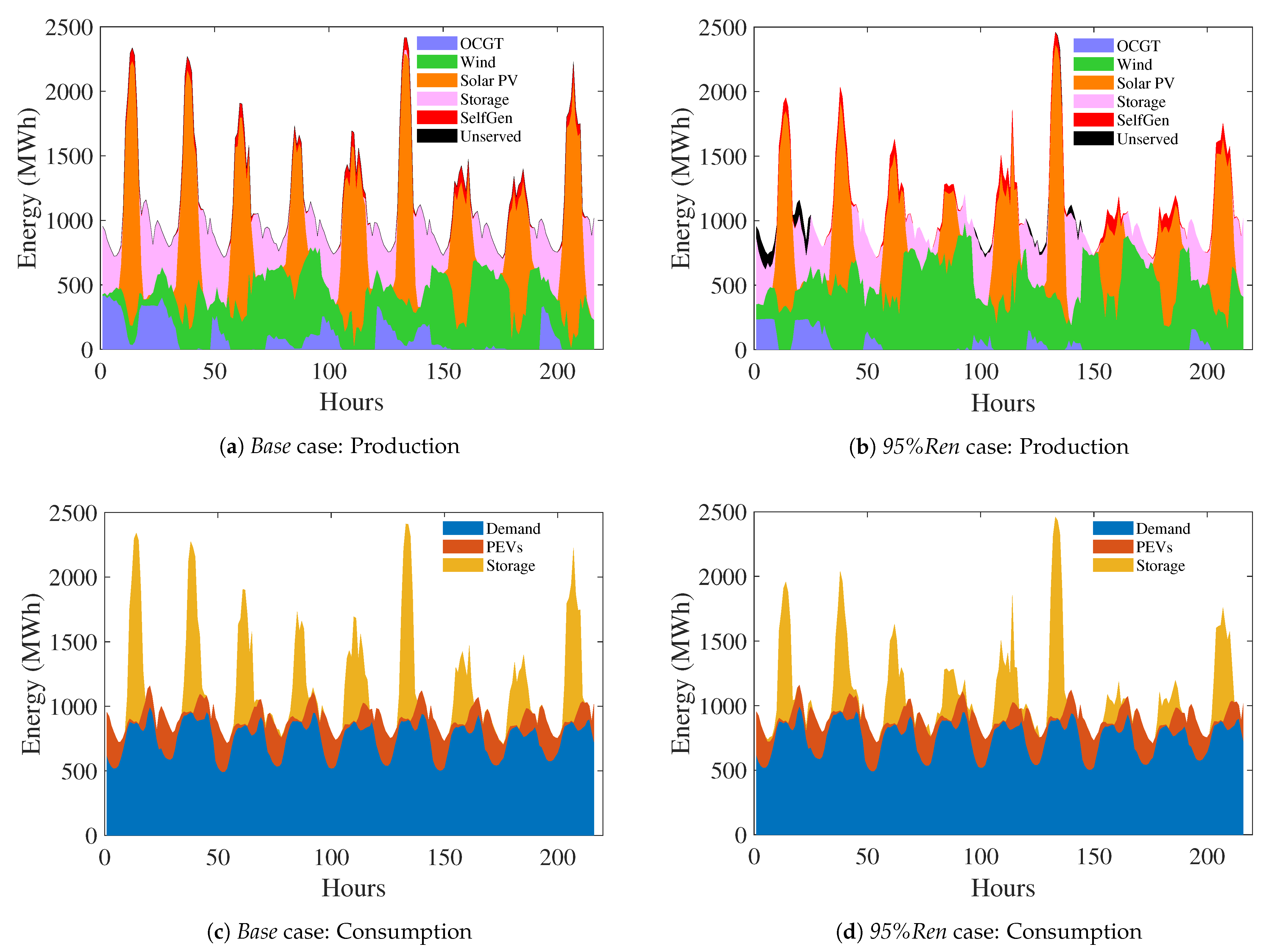
Figure 10 represents the energy production and consumption in each considered day for Base and 95%Ren cases in scenario 7 (see Table 9). As observed in this table, scenario 7 has associated the highest demand and penetration of electric vehicles. In both cases, it is observed that, additionally to the satisfaction of the demand, solar PV energy is mostly used to charge energy storages that are afterwards discharged to procure the demand in periods in which solar PV production is not available. OCGT units, together with wind power units, are used to procure the rest of the demand. The higher participation of wind power units in 95%Ren case is evident. In this case, OCGT units are used in those periods with very low production of wind and solar PV units. However, unserved demand is observed in 95%Ren case in those night-time periods with insufficient production of wind power. It is worth noting that the consumption profile is deeply altered by the charge of storages during midday. It is also interesting to observe that the higher presence of wind power units in 95%Ren case causes a lower usage of storages in all periods, except in those corresponding to days 5 and 6.

Table 16 shows that the up-reserve capacity is exclusively provided by OCGT units, whereas the down-reserve capacity is provided by OCGT and storage units. It is observed that the highest up-reserve capacity is scheduled in 95%Ren case, 579 GW, which is 3.5% higher than that scheduled in Base case. It is also worth noting that OCGT units only provide 31.1% of the down-reserve capacity in 95%Ren case, which is a percentage 35.6% lower than that in Base case. Finally, observe that the up-reserve capacity scheduled in FixedLink case, 556.3 GW, is 0.5 and 3.9% lower than those in Base and 95%Ren cases, respectively.

5.2. Out-of-Sample Analysis Using the AC Model of the System

The performance of the obtained expansion plans has been assessed by implementing an out-of-sample analysis using input data pertaining to year 2019. In this manner, all investment decisions are fixed to their optimal values obtained from solving Base case using the initial set of days generated by using the input data pertaining to 2018. After that, each of the 365 days of year 2019 is simulated to compute how the hourly demand is satisfied in each hour of every day. In order to simulate the steady-state operation of the power system, an optimal AC power flow problem has been solved for each day of the year including active and reactive power flows, losses and voltage magnitudes [71].

Then, hourly demand and power availabilities of wind and solar PV units and solar rooftop facilities in year 2019 have been considered. The demand associated with electric vehicles has been randomly generated for each day using the procedure described in Section 3. As usual, electric vehicle chargers are assumed to operate with power factor equal to 1. The power factor of the rest of loads is assumed to be equal to 0.98. It is considered the conservative criterion stating that only OCGT units are able to provide reactive power. The rest of technologies are considered to operate with power factor equal to 1. The minimum and maximum values of voltage magnitudes are 0.9 and 1.1 times the nominal values.

In order to analyze the operation of the system, two different scenarios are considered:

• Favourable. This scenario corresponds to the case in which all uncertain parameters related to the operation of the system take favourable values from the operation point of view: low demand, low penetration of electric vehicles, high capacity of solar PV self-production facilities and low natural gas prices.
• Unfavourable. In contrast to the Favourable scenario, this scenario corresponds to the case in which all uncertain parameters related to the operation of the system take unfavourable values from the operation point of view: high demand, high penetration of electric vehicles, low capacity of solar PV self-production facilities and high natural gas prices.

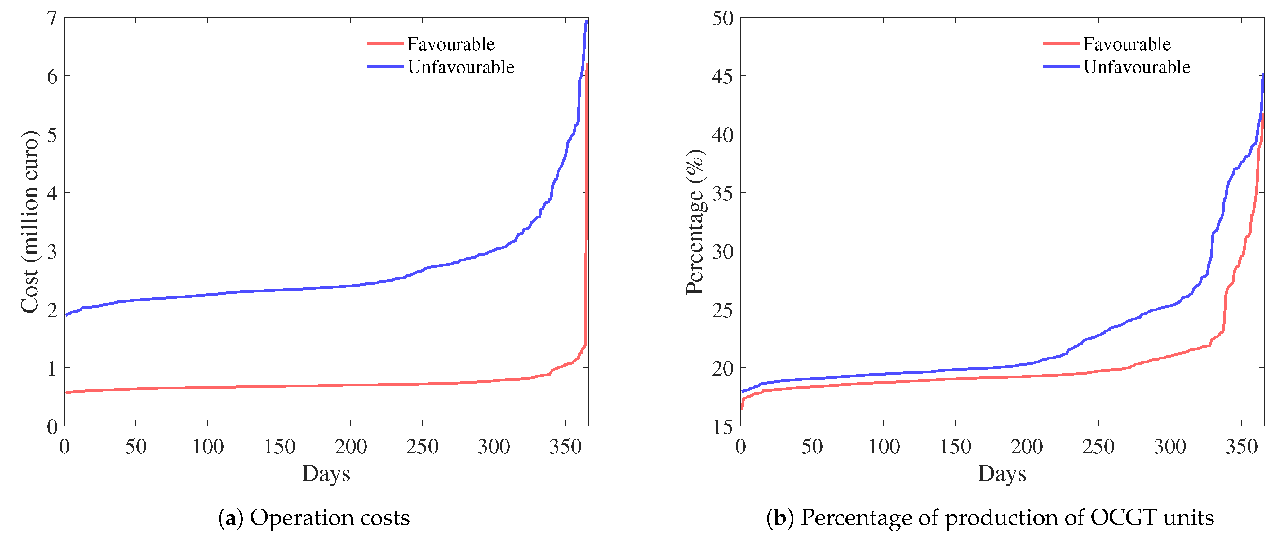
Figure 11 represents the daily operation costs and percentage of demand supplied by OCGT units in each of the scenarios described above considering the investment capacity decisions obtained from the Base case. Note that values are increasingly ordered to facilitate the visualization of the figure. The solution time of each daily simulation is in average equal to 5.3 min, resulting in a total of 32.4 h for each represented curve. The total daily cost in the Favourable scenario is 269 million €, which is 72.4% lower than in Unfavourable scenario, 974 million €. The mean percentage of demand provided by OCGT units in Favourable and Unfavourable scenarios is 20.2% and 22.6%, respectively. Observe that this value is higher than that observed in the DC simulation of year 2018 (Table 15). While the out-of-sample analysis is performed using different input data (year 2019), note that the need for using a DC model in the planning optimization for computational reasons may underestimate the energy production of OCGT units. The reason of this result is twofold: first, the AC modeling considers additional constraints as those related to the reactive power supply or to voltage magnitude limits; second, the AC formulation considered in this study assumes that storages and intermittent power units do not participate in the provision of reactive power. However, it is expected that these technologies be key to provide this resource, and other ancillary services, in renewable-dominated power systems. Finally, note that there is not unserved demand in the Favourable scenario, and only 0.2% in the Unfavourable scenario.

6. Analysis of the Uncertainty Parameters and the Renewable Potentials

This section analyzes the influence of the variation of the uncertain parameters and the renewable potentials in the outcomes of the expansion plan. To that end, uncertain parameters are divided into two groups: (i) investment-related parameters are those parameters that have influence on the investment costs (capital costs of power units and storages), and (ii) operation-related parameters that comprise those parameters which impact the resulting operation costs (demand growth, number of electric vehicles, solar PV self-generation penetration and natural gas prices).

The influence of the renewable and storage potentials on the generation, storage and transmission investment decisions has been analyzed afterwards. For doing that, different renewable potentials ranging between 100% and 25% of the original values have been considered. The expansion plans resulting from each case have been discussed.

6.1. Analysis of the Long-Term Uncertainty

This subsection analyzes the resulting expansion plans for different realizations of the uncertain parameters in the Base case. As stated above, each realization of uncertain parameters is referred as scenario. For the sake of comparison, scenarios are grouped in two different sets depending on their influence on either investment or operation costs. Therefore, the uncertain investment costs of immature generating technologies and storage units are assigned to one group, whereas the rest of parameters (annual demand growth, number of electric vehicles, rooftop solar PV self-production and natural gas prices) are included in the second group.

The investment decisions used to compute the total costs in each scenario are those obtained from solving the Base case, which are reported in the previous section. Note that the investment decisions are first-stage variables and, therefore, they are identical for all considered scenarios (see the decision-making framework represented in Figure 5). On the contrary, operation variables, as the energy produced by installed generating units or the operation of storage units, are second-stage variables which are scenario-dependent. As a result, the cost differences between scenarios are caused only by the variation of the values of the uncertain parameters and system operation variables and not by the implementation of different investment decisions.

6.1.1. Investment-Related Parameters

Table 17. Cost per investment-related scenario (million €).

Scenario	Investment Costs			Operation Costs			Total
	Generation	Storage	Transmission	Day-Ahead	Reserve	Unserved
	Investment	Investment	Investment	Energy	Capacity	Demand
Average	398.6	142.9	4.53	248.6	59.3	0.00	853.9
High GenCost	435.2	142.9	4.53	248.6	59.3	0.00	890.5
Low GenCost	361.9	142.9	4.53	248.6	59.3	0.00	817.3
High StoCost	398.6	204.3	4.53	248.6	59.3	0.00	915.4
Low StoCost	398.6	77.2	4.53	248.6	59.3	0.00	788.2

provides the costs resulting in the following scenarios:

• Average. This scenario corresponds to the scenario in which all uncertain parameters are equal to their expected values.
• High RenCost. This scenario corresponds to the scenario in which all uncertain parameters are equal to their expected values except the investment cost of immature generating units, which is equal to the highest value considered in Table 9.
• Low RenCost. This scenario corresponds to the scenario in which all uncertain parameters are equal to their expected values except the investment cost of immature generating units, which is equal to the lowest value considered in Table 9.
• High StoCost. This scenario corresponds to the scenario in which all uncertain parameters are equal to their expected values except the investment cost of storage units, which is equal to the highest value considered in Table 9.
• Low StoCost. This scenario corresponds to the scenario in which all uncertain parameters are equal to their expected values except the investment cost of storage units, which is equal to the lowest value considered in Table 9.

From the results provided by Table 17 it can be observed that the resulting generation and storage investment costs are highly influenced by the realization of the capital costs of the different technologies. On the contrary, the transmission investment costs as well as the day-ahead energy and reserve capacity costs remain unaltered. If HighGenCost and Average scenarios are compared, it can be observed that the total cost increases 4.3%. In the same manner, LowGenCost scenario, reduces the total cost in the same quantity, 4.3%, with respect to the Average scenario. It is interesting to note that the effect of the variation of the storage investment cost in the total cost is higher than that observed for generating investment costs. Therefore, an increase of 7.2% of the total cost is noticed in HighStoCost scenario. However, the reduction of the cost obtained in LowStoCost scenario with respect to Average scenario is even greater, and it is equal to 7.7%. Based on Table 10, the higher influence of the storage investment costs in the total cost can be explained by the fact that the investment cost of storage units is more uncertain (−45.1%, +54.9) than that of generating units (±10%).

6.1.2. Operation-Related Parameters

Table 18. Cost per operation-related scenario (million €).

Scenario	Investment Costs			Operation Costs			Total
	Generation	Storage	Transmission	Day-Ahead	Reserve	Unserved
	Investment	Investment	Investment	Energy	Capacity	Demand
Average	398.6	142.9	4.53	248.6	59.3	0.00	853.9
High Demand	398.6	142.9	4.53	288.8	60.4	0.00	895.2
Low Demand	398.6	142.9	4.53	213.5	58.1	0.00	817.6
High PEVs	398.6	142.9	4.53	302.8	60.5	0.00	909.3
Low PEVs	398.6	142.9	4.53	199.5	58.1	0.00	803.5
High SelfGen	398.6	142.9	4.53	235.4	58.7	0.00	840.1
Low SelfGen	398.6	142.9	4.53	264.5	59.5	0.00	870.0
High GasPrices	398.6	142.9	4.53	352.0	79.0	0.00	977.0
Low GasPrices	398.6	142.9	4.53	118.8	33.9	0.00	698.7

includes the costs resulting in the following scenarios:

• Average. This scenario corresponds to the scenario in which all uncertain parameters are equal to their expected values.
• High Demand. This scenario corresponds to the scenario in which all uncertain parameters are equal to their expected values except the annual demand growth, which is equal to the highest value considered in Table 9.
• Low Demand. This scenario corresponds to the scenario in which all uncertain parameters are equal to their expected values except the the annual demand growth, which is equal to the lowest value considered in Table 9.
• High PEVs. This scenario corresponds to the scenario in which all uncertain parameters are equal to their expected values except the number of electric vehicles, which is equal to the highest value considered in Table 9.
• Low PEVs. This scenario corresponds to the scenario in which all uncertain parameters are equal to their expected values except the number of electric vehicles, which is equal to the lowest value considered in Table 9.
• High SelfGen. This scenario corresponds to the scenario in which all uncertain parameters are equal to their expected values except the solar PV rooftop capacity, which is equal to the highest value considered in Table 9.
• Low SelfGen. This scenario corresponds to the scenario in which all uncertain parameters are equal to their expected values except the solar PV rooftop capacity, which is equal to the lowest value considered in Table 9.
• High GasPrices. This scenario corresponds to the scenario in which all uncertain parameters are equal to their expected values except the natural gas price, which is equal to the highest value considered in Table 9.
• Low GasPrices. This scenario corresponds to the scenario in which all uncertain parameters are equal to their expected values except natural gas price, which is equal to the lowest value considered in Table 9.

First, it is observed that all generation, storage and transmission investment costs included in Table 18 are identical. As stated above, the reason of this result is that investment decisions are equal for all scenarios and, additionally, the uncertain parameters related to investment costs in all scenarios considered in this analysis are equal to their expected values. In this table we also observe that the natural gas price is the parameter that has the highest influence in the total cost. Despite the fact that only 9.5% of the demand is provided by OCGT units, it is observed that the day-ahead energy cost increases 41.6% in the High GasPrices scenario with respect to that in the Average scenario, whereas the total cost grows 14.4%. The number of electric vehicles and the demand growth have also a great influence in the total costs. It is worth noting that 95% of penetration of electric vehicles (High PEVs scenario) increases the total cost 6.5% with respect to the Average scenario, with a 75% penetration of electric vehicles. In the same manner, the maximum demand (30% higher than the demand in 2018, High Demand scenario) increases the total cost 4.8% with respect to the Average scenario, with a demand 25% higher than the demand in 2018. Finally, the capacity of rooftop solar PV has also a non negligible influence on total cost. In this manner, if only 1% of the potential capacity is used (Low SelfGen scenario), the total cost increases 1.9%. However, if 10% of the potential capacity is exploited (High SelfGen scenario), the total cost decreases 1.6%.

6.2. Influence of Renewable Potentials

The impact of the value of the renewable potential in the obtained results is investigated in this section. To achieve this goal, the Base case is solved considering potential capacities of renewable units less than the original ones.

Table 19. Expected cost as a function of the renewable potentials (million €).

Renewable Potential	Generation Investment	Storage Investment	Transmission Investment	Day-Ahead Energy	Reserve Capacity	Unserved	Total Demand
100%	428.6	142.0	4.53	188.6	45.9	0.00	809.6
75%	375.7	112.2	54.51	308.0	42.4	0.00	892.7
50%	305.7	73.9	53.14	561.5	37.4	0.00	1031.7
25%	221.6	37.3	3.65	947.5	31.8	0.00	1241.8

and

Table 20. Generation and storage capacity to be installed as a function of the renewable potentials (MW).

Renewable Potential	OCGT	Wind	Solar PV	Storage
100%	480.0 (34.1%)	1111.7 (34.4%)	3006.1 (92.1%)	1575.9 (65.7%)
75%	512.0 (36.4%)	1021.3 (42.1%)	2447.2 (100.0%)	1245.4 (51.9%)
50%	672.0 (47.7%)	887.4 (54.9%)	1631.5 (100.0%)	821.6 (34.2%)
25%	896.0 (63.6%)	638.3 (79.0%)	815.7 (100.0%)	414.1 (17.3%)

provide the expected cost and the capacity installed for different potential values. The potentials are denoted in percentage with respect to the original values indicated in Table 2 and Table 3. As expected, it is observed that the total cost increases significantly as the potential capacity of renewable units decreases. For instance, the total cost increases 53.4% if the renewable potential decreases from its initial value (100%) to 25%. This cost increase is mainly due to the increment of the day-ahead energy costs, which grow 402.4%, from 188.6 M€ to 947.5 M€. A portion of this increment is compensated by the reduction of generation and storage investment costs, which are reduced 48.3 and 73.7%, respectively.

Table 20 shows that the generation capacity of OCGT units increases significantly as the renewable potential decreases. If the potential decreases up to 25%, the capacity installed of OCGT units increases 86.7%. It is also interesting to note that there is not any case in which the installed capacity of wind power reaches the potential capacity, whereas the solar PV capacity installed is equal to the capacity for potentials less than or equal to 75% of the original values. Finally, it is remarkable the effect of reducing the renewable potential in the installation of storage units. If the renewable potential decreases up to 25%, the capacity installed of storage units decreases 73.7%. Therefore, we can conclude that the installation of storage units is closely tied to the presence of renewable units.

7. Conclusions

This paper has proposed a novel generation, storage and transmission expansion formulation considering a number of uncertain parameters: investment costs of renewable and storage units, demand growth, penetration of electric vehicles, solar PV self-production capacity and natural gas prices. The proposed procedure has been applied to the isolated power system of Las Palmas (Spain) for 2050. The proposed generation, storage and transmission capacity to be installed has been determined by solving a two-stage stochastic programming problem, where the operation of the power system has been simulated by modeling the day-ahead energy and reserve capacity markets in a set of characteristic days.

Several case studies have been analyzed considering a (i) base case, (ii) a minimum percentage of renewable generation, (iii) the installation of a transmission line between GC and LZ-FV systems and (iv) different renewable capacity potentials. Furthermore, the impact of the realization of different scenarios has been tested in the obtained expansion plan. Finally, the performance of the resulting power system has been assessed by solving an out-of-sample analysis using the AC model of the resulting power system.

Based on the numerical results presented in the case study, the following conclusions can be made:

• The highest investment costs are associated with the investments in new generation capacity. On the contrary, investments in transmission lines are significantly smaller.
• The enforcement of a strong minimum requirement of non-thermal production (95%) causes higher investment costs and lower operation costs. For instance, generation and storage investments costs increase 66.4 and 20.6% with respect to the base case.
• The reserve capacity cost increases 9.5% if a minimum of 95% of non-thermal production is enforced. The up-reserve capacity is exclusively procured by OCGT units, whereas the down-reserve capacity is provided by OCGT and storage units.
• The case with a minimum of 95% of non-thermal production has associated 1.42% of unserved demand.
• The construction of a transmission link between GC and LZ-FV power systems cannot be justified solely by economic reasons. If this link is built, a 8.5% reduction of the investment cost in storage units is achieved.
• The generation technology most used is solar PV, which is installed 92.1% over its potential and produces 42.2% of the total demand.
• OCGT units only satisfy 9.5% of the total demand and they are at operation only 1967.7 equivalent hours per year.
• The investments in transmission lines grow as the renewable power penetration increases (56.3% in case with 95% of non-thermal production).
• The natural gas price is the uncertain parameter that has the highest influence in the total cost. It is observed that the day-ahead energy cost increases 41.6% if natural gas prices are high with respect to the case in which natural gas prices are equal to their expected value.
• The number of electric vehicles and the demand growth have also a great influence in the total operation costs. It is worth noting that 95% of penetration of electric vehicles increases the total cost 6.5% with respect to the case with 75% penetration of electric vehicles.
• If the installed capacity of solar PV rooftop facilities increases from 5 to 10%, the total operation cost decreases 1.6%.
• The total cost increases 53.4% if the renewable potential decreases up to 25% of the nominal value. The installation of storage units is highly dependent on the presence of renewable units. If the renewable potential decreases up to 25%, the capacity installed of storage units decreases 73.7%.
• The results of the AC out-of-sample analysis indicate that the usage of the DC modeling in the formulation of the capacity expansion problem may underestimate the production of OCGT units if storages and intermittent power units are not considered to provide reactive power.

Future research lines are the formulation of the GSTEP considering: (i) system frequency limits and the provision of virtual inertia by inverter-connected generation and storage units, and (ii) combined-cycle gas turbines with a precise modeling of their different operation modes.

References

1. European Commission. Energy Roadmap 2050; Publications Office of the European Union: Luxembourg, Belgium, 2012; ISBN 978-92-79-21798-2. [Google Scholar] [CrossRef]
2. Dunn, B.; Kamath, H.; Tarascon, J.-M. Electrical Energy Storage for the Grid: A Battery of Choices. Science 2011, 334, 928–935. [Google Scholar] [CrossRef] [PubMed] [Green Version]
3. Red Eléctrica de España. Available online: https://www.ree.es/en/activities/canary-islands-electricity-system (accessed on 8 May 2021).
4. Calero, R.; Carta, J.A. Action plan for wind energy development in the Canary Islands. Energy Policy 2004, 32, 1185–1197. [Google Scholar] [CrossRef]
5. Santana-Sarmiento, F.; Álamo-Vera, F.R.; De Saá-Pérez, P. A resource-based view of competitiveness in the wind energy sector: The case of Gran Canaria and Tenerife. Appl. Sci. 2019, 9, 1263. [Google Scholar] [CrossRef] [Green Version]
6. Padrón, S.; Medina, J.F.; Rodríguez, A. Analysis of a pumped storage system to increase the penetration level of renewable energy in isolated power systems. Gran Canaria: A case study. Energy 2011, 36, 6753–6762. [Google Scholar] [CrossRef]
7. Bueno, C.; Carta, J.A. Technical-economic analysis of wind-powered pumped hydrostorage systems. Part II: Model application to the island of El Hierro. Sol. Energy 2005, 78, 396–405. [Google Scholar] [CrossRef]
8. Cabrera, P.; Lund, H.; Carta, J.A. Smart renewable energy penetration strategies on islands: The case of Gran Canaria. Energy 2018, 162, 421–443. [Google Scholar] [CrossRef] [Green Version]
9. Gils, H.C.; Simon, S. Carbon neutral archipelago—100% renewable energy supply for the Canary Islands. Appl. Energy 2017, 188, 342–355. [Google Scholar] [CrossRef] [Green Version]
10. Carrión, M.; Domínguez, R.R.; Zárate-Minano, R. Influence of the controllability of electric vehicles on generation and storage capacity expansion decisions. Energy 2019, 189, 116156. [Google Scholar] [CrossRef]
11. Cañas-Carretón, M.; Carrión, M. Generation capacity expansion considering reserve provision by Wind Power Units. IEEE Trans. Power Syst. 2020, 35, 4564–4573. [Google Scholar] [CrossRef]
12. Schallenberg-Rodríguez, J. Photovoltaic techno-economical potential on roofs in regions and islands: The case of the Canary Islands. Methodological review and methodology proposal. Renew. Sustain. Energy Rev. 2013, 20, 219–239. [Google Scholar] [CrossRef]
13. Santamarta, J.C.; Jarabo, F.; Rodríguez-Martín, J.; Arraiza, M.P.; López, J.V. Analysis and Potential of Use of Biomass Energy in Canary Islands, Spain. IERI Procedia 2014, 8, 136–141. [Google Scholar] [CrossRef] [Green Version]
14. Ramos-Real, F.J.; Moreno-Piquero, J.C.; Ramos-Henríquez, J.M. The effects of introducing natural gas in the Canary Islands for electricity generation. Energy Policy 2007, 35, 3925–3935. [Google Scholar] [CrossRef]
15. Marrero, G.A.; Ramos-Real, F.J. Electricity generation cost in isolated system: The complementarities of natural gas and renewables in the Canary Islands. Renew. Sustain. Energy Rev. 2010, 14, 2808–2818. [Google Scholar] [CrossRef] [Green Version]
16. Semshchikov, E.; Negnevitsky, M.; Hamilton, J.; Wang, X. Cost-Efficient Strategy for High Renewable Energy Penetration in Isolated Power Systems. IEEE Trans. Power Syst. 2020, 35, 3719–3728. [Google Scholar] [CrossRef]
17. Silva, A.R.; Estanqueiro, A. Optimal Planning of Isolated Power Systems with near 100% of Renewable Energy. IEEE Trans. Power Syst. 2020, 35, 1274–1283. [Google Scholar] [CrossRef]
18. Ringkjøb, H.K.; Haugan, P.M.; Nybø, A. Transitioning remote Arctic settlements to renewable energy systems—A modelling study of Longyearbyen, Svalbard. Appl. Energy 2020, 258, 114079. [Google Scholar] [CrossRef]
19. Kaldellis, J.K. Supporting the Clean Electrification for Remote Islands: The Case of the Greek Tilos Island. Energies 2021, 14, 1336. [Google Scholar] [CrossRef]
20. Conejo, A.J.; Baringo, L.; Kazempour, S.J.; Siddiqui, A.S. Investment in Electricity Generation and Transmission, 1st ed.; Springer: Berlin/Heidelberg, Germany, 2016; ISBN 978-3-319-29501-5. [Google Scholar]
21. Alvarez, J.; Ponnambalam, K.; Quintana, V.H. Transmission expansion under risk using stochastic programming. In Proceedings of the 9th International Conference on Probabilistic Methods Applied to Power Systems, PMAPS, Beijing, China, 16–20 October 2016; Volume 22, pp. 1369–1378. [Google Scholar] [CrossRef]
22. Roh, J.H.; Shahidehpour, M.; Wu, L. Market-Based Generation and Transmission Planning With Uncertainties. IEEE Trans. Power Syst. 2009, 24, 1587–1598. [Google Scholar] [CrossRef]
23. Baringo, L.; Conejo, A.J. Transmission and wind power investment. IEEE Trans. Power Syst. 2012, 27, 885–893. [Google Scholar] [CrossRef]
24. Pozo, D.; Sauma, E.; Contreras, J. A three-level static MILP model for generation and transmission expansion planning. IEEE Trans. Power Syst. 2013, 28, 202–210. [Google Scholar] [CrossRef]
25. Domínguez, R.; Conejo, A.J.; Carrión, M. Toward fully renewable electric energy systems. IEEE Trans. Power Syst. 2015, 30, 316–326. [Google Scholar] [CrossRef]
26. Baringo, L.; Baringo, A. A stochastic adaptive robust optimization approach for the generation and transmission expansion planning. IEEE Trans. Power Syst. 2018, 33, 792–802. [Google Scholar] [CrossRef]
27. Roldán, C.; Sánchez de la Nieta, A.A.; García-Bertrand, R.; Mínguez, R. Robust dynamic transmission and renewable generation expansion planning: Walking towards sustainable systems. Int. J. Electr. Power Energy Syst. 2018, 96, 52–63. [Google Scholar] [CrossRef] [Green Version]
28. Liu, Y.; Sioshansi, R.; Conejo, A.J. Multistage stochastic investment planning with multiscale representation of uncertainties and decisions. IEEE Trans. Power Syst. 2018, 33, 781–791. [Google Scholar] [CrossRef]
29. Moghaddam, S.Z. Generation and transmission expansion planning with high penetration of wind farms considering spatial distribution of wind speed. Int. J. Electr. Power Energy Syst. 2019, 106, 232–241. [Google Scholar] [CrossRef]
30. Chen, X.; Lv, J.; McElroy, M.B.; Han, X.; Nielsen, C.P.; Wen, J. Power system capacity expansion under higher penetration of renewables considering flexibility constraints and low carbon policies. IEEE Trans. Power Syst. 2018, 33, 6240–6253. [Google Scholar] [CrossRef]
31. Asadi Majd, A.; Farjah, E.; Rastegar, M. Composite generation and transmission expansion planning toward high renewable energy penetration in Iran power grid. IET Renew. Power Gener. 2020, 14, 1520–1528. [Google Scholar] [CrossRef]
32. Domínguez, R.; Carrión, M.; Conejo, A.J. Influence of the number of decision stages on multi-stage renewable generation expansion models. Int. J. Electr. Power Energy Syst. 2021, 126. [Google Scholar] [CrossRef]
33. JRC. ETRI 2014: Energy Technology Reference Indicator Projections for 2010–2050; European Commission Joint Research Centre: Ispra, Italy, 2014. [Google Scholar] [CrossRef]
34. International Group of Liquefied Natural Gas Importers. The LNG Industry Annual Report. 2021. Available online: https://giignl.org/system/files/publication/giignl_-_2020_annual_report_-_04082020.pdf (accessed on 8 May 2021).
35. BOE 738/2015. Boletin Oficial Del Estado. Available online: https://www.boe.es/buscar/doc.php?id=BOE-A-2015-8646 (accessed on 8 May 2021).
36. Ministerio de Industria, Turismo y Comercio. Planificación Energética. Plan de Desarrollo de La Red de Transporte de Energía Eléctrica 2015–2020; Technical Report; Subdirección General de Desarrollo Normativo, Informes y Publicación: Madrid, Spain, 2015. (In Spanish) [Google Scholar]
37. Gobierno de Canarias. Anuario Energético de Canarias 2018; Technical Report; Instituto Canario de Estadística: Canarias, Spain, 2019. [Google Scholar]
38. Gobierno de Canarias. Anuario del Sector Eléctrico de Canarias 2019; Technical Report; Gobierno de Canarias: Santa Cruz de Tenerife, Spain, 2020. [Google Scholar]
39. Gobierno de Canarias. IDECanarias Visor 4.5.1. Available online: https://visor.grafcan.es/visorweb/# (accessed on 8 May 2021).
40. Mapas de Gran Canaria (Visor 4.5 OL IDEGranCanaria). Available online: https://visor.idegrancanaria.es/# (accessed on 8 May 2021).
41. Rodríguez Bordón, J.D. Estudio Sobre las Interconexiones de los Sistemas Eléctricos de las Islas Canarias. Ph.D. Thesis, Universidad de Las Palmas de Gran Canaria, Las Palmas de Gran Canaria, Spain, 2011. [Google Scholar]
42. BOE. Gobierno de España—Documento BOE-A-2006-9613. 2006. Available online: https://www.boe.es/buscar/doc.php?id=BOE-A-2006-9613 (accessed on 8 May 2021).
43. AENOR. UNE 21018:1980 Bare Aluminium Conductor Standardization for over Head Power Lines; AENOR: Madrid, Spain, 1980. [Google Scholar]
44. Gobierno de Canarias. Boletín Oficial de Canarias—2021/023. Miércoles 3 de Febrero de 2021—Anuncio 559; Gobierno de Canarias: Santa Cruz de Tenerife, Spain, 2021. [Google Scholar]
45. Gröwe-Kuska, N.; Heitsch, H.; Römisch, W. Scenario reduction and scenario tree construction for power management problems. In Proceedings of the IEEE Bologna Power Technology Conference Bologna, Bologna, Italy, 23–26 June 2003. [Google Scholar]
46. Spanish Market Operator (OMIE). Available online: http://www.omie.es (accessed on 8 May 2021).
47. NREL-National Renewable Energy Laboratory, Western Wind and Solar Integration Study. 2010. Available online: https://goo.gl/NvUBK8 (accessed on 8 May 2021).
48. Fang, J.; Li, H.; Tang, Y.; Blaabjerg, F. Distributed Power System Virtual Inertia Implemented by Grid-Connected Power Converters. IEEE Trans. Power Electron. 2018, 33, 8488–8499. [Google Scholar] [CrossRef] [Green Version]
49. Peña Asensio, A.; Gonzalez-Longatt, F.; Arnaltes, S.; Rodríguez-Amenedo, J.L. Analysis of the Converter Synchronizing Method for the Contribution of Battery Energy Storage Systems to Inertia Emulation. Energies 2020, 13, 1478. [Google Scholar] [CrossRef] [Green Version]
50. Wu, Z.; Gao, D.W.; Zhang, H.; Yan, S.; Wang, X. Coordinated Control Strategy of Battery Energy Storage System and PMSG-WTG to En-hance System Frequency Regulation Capability. IEEE Trans. Sustain. Energy 2017, 8, 1330–1343. [Google Scholar] [CrossRef]
51. Fernández-Guillamón, A.; Gómez-Lázaro, E.; Muljadi, E.; Molina-García, Á. Power systems with high renewable energy sources: A review of inertia and frequency control strategies over time. Renew. Sustain. Energy Rev. 2019, 115, 109369. [Google Scholar] [CrossRef] [Green Version]
52. Hoyland, K.; Wallace, S.W. Generating scenario trees for multistage decision problems. Manag. Sci. 2001, 47, 295–307. [Google Scholar] [CrossRef] [Green Version]
53. International Energy Agency. World Energy Outlook 2016. 2016. Available online: https://www.iea.org/weo/ (accessed on 8 May 2021).
54. Cole, W.; Frazier, A.W. Cost Projections for Utility-Scale Battery Storage; National Renewable Energy Laboratory: Golden, CO, USA, 2019. [Google Scholar]
55. Global Energy Transformation: A Roadmap to 2050. IRENA. Available online: https://www.irena.org/publications/2019/Apr/Global-energy-transformation-A-roadmap-to-2050-2019Edition (accessed on 8 May 2021).
56. Electrification Futures Study: Scenarios of Electric Technology Adoption and Power Consumption for the United States. Available online: https://www.nrel.gov/analysis/electrification-futures.html (accessed on 8 May 2021).
57. International Energy Agency. Energy Technology Perspectives; Annex H: Rooftop Solar PV Potential in Cities; International Energy Agency: Paris, France, 2016; ISBN 978-92-64-25234-9. [Google Scholar]
58. Izquierdo, S.; Rodrigues, M.; Fueyo, N. A method for estimating the geographical distribution of the available roof surface area for large-scale photovoltaic energy-potential evaluations. Sol. Energy 2008, 82, 929–939. [Google Scholar] [CrossRef]
59. Huld, T.; Bodis, K.; Pinedo, I.; Dunlop, E.; Taylor, N.; Jäger-Waldau, A. The Rooftop Potential for PV Systems in the European Union to Deliver the Paris Agreement; Joint Research CentreDirectorate; European Commission: Brussels, Belgium, 2018. [Google Scholar]
60. ECF. Roadmap 2050: A Practical Guide to a Prosperous, Low-Carbon Europe. Full Documentation; European Climate Foundation: Brussels, Belgium, 2010. [Google Scholar] [CrossRef]
61. Instituto Nacional de Estadística. Available online: https://www.ine.es/ (accessed on 8 May 2021).
62. United Nations. Growing at a Slower Pace, World Population Is Expected to Reach 9.7 Billion in 2050 and Could Peak at Nearly 11 Billion around 2100: UN Report. Available online: https://population.un.org/wpp/Publications/Files/WPP2019_PressRelease_EN.pdf (accessed on 8 May 2021).
63. IEA. Global EV Outlook 2019; IEA: Paris, France, 2019; Available online: https://www.iea.org/reports/global-ev-outlook-2019 (accessed on 8 May 2021).
64. Carrión, M.; Zárate-Miñano, R.; Domínguez, R. Integration of Electric Vehicles in Low-Voltage Distribution Networks Considering Voltage Management. Energies 2020, 13, 4125. [Google Scholar] [CrossRef]
65. Mobility Report for Residents in Spain (MOVILIA). Available online: https://www.mitma.gob.es/informacion-para-el-ciudadano/informacion-estadistica/movilidad/encuesta-de-movilidad-de-las-personas-residentes-en-espana (accessed on 8 May 2021).
66. Duic, N.; Štefanic, N.; Lulic, Z.; Krajacic, G.; Puksec, T.; Novosel, T. EU28 Fuel Prices for 2015, 2030 and 2050. Heat Roadmap Europe 2050. 2017. Available online: https://heatroadmap.eu/ (accessed on 8 May 2021).
67. Morales, J.M.; Pineda, S.; Conejo, A.J.; Carrion, M. Scenario Reduction for Futures Market Trading in Electricity Markets. IEEE Trans. Power Syst. 2009, 24, 878–888. [Google Scholar] [CrossRef]
68. Domínguez, R.; Carrión, M. Impact of the Demand Side Management in the Planning and Operations Towards 2050. In Proceedings of the 16th International Conference on the European Energy Market (EEM19), Ljubljana, Slovenia, 18–20 September 2019. [Google Scholar]
69. Rosenthal, R.E. GAMS, a User’s Guide; GAMS Development Corp: Washington, DC, USA, 2008; Available online: https://docs.lib.purdue.edu/alsinternal/69/ (accessed on 8 May 2021).
70. The IBM CPLEX. Available online: https://www.ibm.com/analytics/cplex-optimizer (accessed on 8 May 2021).
71. Gómez Expósito, A.; Conejo, A.J.; Cañizares, C. (Eds.) Electric Energy Systems: Analysis and Operation; The Electric Power Engineering Series; CRC Press: Boca Raton, FL, USA, 2009. [Google Scholar]
Figure 1. Location of Canary Islands.
Energies 14 03317 g001
Figure 2. Single-line diagram of Las Palmas power system.
Energies 14 03317 g002
Figure 3. Wind and solar PV availabilities.
Energies 14 03317 g003
Figure 4. Demand.
Energies 14 03317 g004
Figure 5. Decision-making framework.
Energies 14 03317 g005
Figure 6. Self-generation.
Energies 14 03317 g006
Figure 7. Modeling of the charge of electric vehicles.
Energies 14 03317 g007
Figure 8. Example of charging profiles of EVs.
Energies 14 03317 g008
Figure 9. Electric vehicle demand.
Energies 14 03317 g009
Figure 10. Energy produced and consumed in a scenario with high demand and high penetration of electric vehicles (scenario 7 described in Table 9).
Energies 14 03317 g010
Figure 11. Out-of-sample results.
Energies 14 03317 g011