Transportation-Mission-Based Optimization of Heterogeneous Heavy-Vehicle Fleet Including Electrified Propulsion

Abstract

Commercial-vehicle manufacturers design vehicles to operate over a wide range of transportation tasks and driving cycles. However, certain possibilities of reducing emissions, manufacturing and operational costs from end vehicles are neglected if the target range of transportation tasks is narrow and known in advance, especially in case of electrified propulsion. Apart from real-time energy optimization, vehicle hardware can be meticulously tailored to best fit a known transportation task. As proposed in this study, a heterogeneous fleet of heavy-vehicles can be designed in a more cost- and energy-efficient manner, if the coupling between vehicle hardware, transportation mission, and infrastructure is considered during initial conceptual-design stages. To this end, a rather large optimization problem was defined and solved to minimize the total cost of fleet ownership in an integrated manner for a real-world case study. In the said case-study, design variables of optimization problem included mission, recharging infrastructure, loading–unloading scheme, number of vehicles of each type, number of trips, vehicle-loading capacity, selection between conventional, fully electric, and hybrid powertrains, size of internal-combustion engines and electric motors, number of axles being powered, and type and size of battery packs. This study demonstrated that by means of integrated fleet customization, battery-electric heavy-vehicles could strongly compete against their conventional combustion-powered counterparts. The primary focus has been put on optimizing vehicle propulsion, transport mission, infrastructure and fleet size rather than routing.

1. Introduction

Commercial vehicles are, traditionally, designed to perform a wide range of transportation tasks. However, vehicle optimality is often compromised depending on how the vehicle is desired to be used. Although consumers partly recognize what vehicle type they need to purchase, corresponding operational costs cannot be easily foreseen, and the selected vehicle, therefore, might not be best-suited to perform the assigned task. A major challenge faced by commercial-vehicle manufacturers concerns prediction of transportation needs and corresponding delivery of optimized vehicles.

Normally, a transportation company selects a set of vehicles and plans routes to meet present transportation demands. As [1] argues, a single transportation-related problem formulation cannot reflect all real-life applications, and that it does not make sense to include detailed vehicle and routing aspects in strategic fleet-management decisions owing to the inherent high level of uncertainty. However, if a detailed description of repetitive transportation assignments and operational environment can be obtained via communication with future customers, detailed design of vehicle and transportation aspects could be undertaken in an integrated manner by vehicle manufacturers.

Environmental, technical, logistic, and financial factors as well as energy supply and infrastructure have especially a major impact on electromobility, as reported by [2,3,4]. As concluded by [5], profitability is the primary reason for major transportation companies to consider the switch-over to electrification. They suggest measures to increase profitability by pointing out that further research is needed to investigate development of a systematic approach.

Vehicle customization can be a part of the solution, nevertheless, it is not a new objective of commercial-vehicle manufacturers. For example, the Global Truck Application [6] or Global Transport Application (GTA) [7] has already been developed to provide descriptions of vehicle utilization and operational environment. The tool could be used for vehicle customization and tailoring/optimization of hardware components to suit the operational environment and transportation assignments. Furthermore, such a tool can be incorporated along with a more detailed description of the distribution network characterized by nodes, demands, and available routes, to design even better customized vehicles. Based on such a description, this study proposes design of a heterogeneous fleet of commercial vehicles, trucks, and long combination heavy-vehicles together with infrastructure to facilitate zero emission and achievement of a profitable business by minimization of the total cost of ownership (TCO). As regards the environmental, technical, logistic, financial, energy supply and infrastructure factors, in this study, it is proposed that they are interconnected, and for successful deployment of new transportation technologies, all relevant factors must be considered together in a vehicle-transportation optimization/customization process.

In the proposed optimization problem, vehicle-design variables include vehicle size; type of propulsion system—a choice between conventional, plug-in hybrid, and fully electric vehicles; size of internal combustion engine (ICE); size and type of electric motors and battery packs; etc. Since integrated design of vehicle-transportation systems is considered in this study, boundaries within which vehicle design can be affected were carefully set. Therefore, route selection (among a small set of available routes), fleet size and composition, loading–unloading scheme, recharging strategy, position of charging stations, and number of trips have also been considered as transportation design variables. The suggested strategy can be employed as a systematic approach to increase the profitability of electric freight vehicles.

Another important area of development is logistics and routing management systems. They typically suffer from lack of proper data supply [8]. For this, telematics can play an significant role in the future development [9]. This study assumes that proper data is supplied so that the sets of transportation design variables are known prior to the optimization.

The major contribution of this study to the literature lies in demonstration of coupling between logistics, routing, vehicle-hardware design, and infrastructure design. Such optimization has a strong essence of multi-criteria decisions [10], for which, this study utilizes the fleet TCO as a cost function considering the service life of vehicles. TCO is usually used for measuring competitiveness between different vehicle powertrain solutions, for example in works done by [4,11]. TCO reflects differences between fixed and operational costs of different vehicle-hardware setups. Here, TCO includes the driver wage, fuel costs, electrical energy costs, maintenance, tax, insurance, battery degradation and replacements, loading–unloading costs, recharging-station installation, and depreciation of vehicle components. For calculating energy consumption, an on-road dynamic vehicle model has been solved considering road topography, and vehicle starts and stops. In addition, TCO was observed to be nonlinear depending on number of vehicles, since battery recharging and loading–unloading infrastructures could be shared among vehicles. This study especially demonstrates the competitiveness between optimized conventional, fully electric, and plug-in hybrid commercial heavy-vehicle combinations assigned to transportation missions of different characteristics, and discusses different contributing factors such as payload, battery size, charging power, battery quality, number of vehicles, and vehicle utilization level. In addition, sensitivity analyses have been performed to demonstrate the effects of different vehicle hardware setup on TCO and its cost indicators.

Moreover, long heavy-vehicle combinations are included in the list of vehicle-size candidates, since they demonstrate roughly 15–20% reduction in emissions compared to conventional tractor semi-trailer combinations as reported by [12]. In this study, it has been demonstrated that using long heavy-vehicle combinations in a heterogeneous fleet results in an approximate 53% reduction in TCO compared to a homogeneous fleet comprising rigid trucks.

This paper is organized as follows. Section 2 provides a background on existing literature. Section 3 demonstrates a general description of the optimization problem. Section 4 outlines the methodology employed for solving the problem by dividing it into small optimization subproblems. In Section 5, a case-study problem has been solved using the proposed methodology and the related results have been presented. This section is followed by sections on associated discussions, and conclusions drawn from this study. Appendices provide more information about the method, case study, vehicle models and used data.

2. Background

2.1. Research Question

In this study, the vehicle design search space is very large and the route search space is small. On the contrary, a class of problems, where the route search space is very large and the vehicle design search space is very small, relates to vehicle routing problems (VRPs). Numerous researches aimed at determining the optimum route and size of a fleet have been performed, wherein the vehicle hardware setup (e.g., powertrain) is already known [1,13,14,15]; therefore, the possibility of further reduction in costs or emissions via combined hardware-design and fleet optimization has not been considered. Likewise, several studies have been performed concerning VRP and heterogeneous VRP (HVRP), wherein differently sized and powered vehicles are dealt with. These include works by [16,17,18,19,20,21]. In all these extant studies, six or less vehicle types have been tested and about three route–vehicle aspects have been simultaneously investigated, such as vehicle capacity, source of power—electrical or thermal, battery size, charging-station location, and charging power.

The same argument holds for the study reported by [22], wherein VRPs concerning electric and hybrid vehicles have been tackled considering the availability of charging stations. The determined shortest energy-efficient routes may differ depending on battery usage, hybrid-powertrain control, and location of charging stations, thereby motivating simultaneous design optimization of vehicles, charging stations, battery size, and routing. Utilization of charging stations at depots or consumer locations is motivated by the fact that it saves cost and time compared to using public-scarce charging stations [17]. Moreover, more cost and time can be saved if charging can be accomplished during the same time as performing service operations, such as loading and unloading [23]. Therefore, this study included the cost of infrastructure, i.e., the cost of LU and charging stations, in the calculation of the TCO for the given transportation network.

In the classical VRPs, each customer is visited by only a single vehicle. Split pick-ups and deliveries, wherein a node can be visited by several vehicles of the same or different types to fulfil consumer demand has been investigated by [24]. Demand of each node is defined by the pick-up/delivery of freight from/to that node. Moreover, the demand may exceed vehicle capacity [25], as the case of this study.

Another class of related optimization problems refer to the fleet-vehicle replacement optimization framework, wherein routes, number, and loading capacities of vehicles are initially known [26]. Such a framework replaces the existing conventional old fleet of vehicles with new and electric vehicles neglecting the interconnection between fleet size, route, infrastructure, battery size, and vehicle powertrain.

Electrification of road freight transport is a path towards green transportation. However, the profitability and feasibility of deploying battery electric heavy vehicles remains a concern. The weight and volume of goods, operating range, payload, utilization level, purchase cost, charging infrastructure, battery life, energy consumption, available routes, average speed, and logistics are among the factors that affect the profitability of battery electric heavy vehicles, according to [2,3,5,11,20,23,26,27,28,29,30,31,32]. TCO provides a good means of estimating profitability and is used for comparative analysis of the competitive technologies [3,5,20,23,26,27,28,29,33,34,35,36,37,38,39]. Literature suggests that vehicle customization based on the use case helps profitability of the battery electric heavy vehicles. However, the influence of such a customization on TCO is not studied in the literature. Moreover, the driver cost is neglected in TCO calculation of the electric freight vehicles in the literature, and thus additional cost related to the waiting time for charging during operation is omitted. Similarly, the trade-offs between the driver cost and charging time, charging power and cost, battery degradation, and loading–unloading time and cost are neglected in TCO calculations of freight vehicles. In addition, TCO analysis of battery electric trucks in the literature is limited to trucks weighing less than 12 tons.

This study tried to fill the above gaps and is the extension of the work done by [11] to include a transportation network rather than a single mission comprising two nodes. The vehicle-infrastructure optimization was studied in [11], where it was shown that such an optimization helps competitiveness of battery electric heavy vehicles against conventional counterparts, while transportation task included only one vehicle type and two pickup and delivery nodes. TCO comparison of different battery electric vehicles by itself does not reflect the profitability, due to the performance constraint imposed by the range and power of batteries. Therefore, this problem can be overcome by optimizing vehicle-infrastructure, e.g., by sizing the batteries for a given transportation scenario. The problem of vehicle-infrastructure design of a vehicle fleet, including route selection coupled with powertrain-component tailoring was first defined in [40]. In such an optimization problem, numbers of each designed-vehicle type on each route were selected as design variables. That study showed that the design of electrified propulsion was influenced by the fleet composition.

2.2. Methodology

Among different formulations of a route set in HVRP [15], the route set defined using the set partitioning method, as reported in [41,42,43], best suited the objectives of the proposed study, since cyclic routes defined using the set partitioning formulation demonstrate great relevance to mission definitions or driving cycles used in the tailoring of vehicle powertrain components.

Another class of problems are fleet-size and mix-vehicle routing problem (FSMVRP), extensively studied in the literature. A heterogeneous or mixed fleet refers to vehicles with different payload capacities [15,44]. Moreover, there exists rich literature [1,15] concerning HVRP solutions obtained through use of heuristic and exact methods. An exact method for solving HVRPs of different classes, based on set partitioning formulation, is presented in [43].

In this study, vehicles are different in the powertrain design in addition to the vehicle capacity. Depending on vehicle-design parameters and their corresponding range, i.e., continuous or discrete, the total number of different vehicle types might amount to billions or be infinite. The resulting FSMVRP can, therefore, be very large. Furthermore, addition of every single decision variable (for example, charging-station location, loading–unloading scheme at each node and number of trips) to the routing problem adds a layer of complexity making the structure of the problem different from FSMVRP. Therefore, the applicability of the above methods on very large or infinite number of vehicle types and many layers of complexity needs further investigation. However, for the presented case study comprising a small transportation network, the proposed method in this study yields sufficiently a good solution within the objectives of this study.

To our knowledge, there is no similar work in the literature where many aspects of vehicle design and transportation network, including charging-station-location problem and loading–unloading schemes, were optimized simultaneously. However, the literature reports an extensive work in vehicle routing problems where the vehicle type search space is small and the route search space is very large, in contrast to the problem presented in this paper, where vehicle type search space is very large and the route search space is small. For example, for a small number of vehicle types, in [45], the Benders decomposition approach was employed for solving the charging-station-location problem. Benders decomposition, introduced by [46], has also been demonstrated to be useful in solving heterogeneous vehicle routing problems, wherein relatively a large set of vehicle types are allowed in the fleet [47], the idea being to initialize the optimization problem with a small set of added decision variables whilst fixing all others. Subsequently, the set of fixed decision variables is iteratively improved along with major routing decision variables by solving each optimization subproblem. In case of a rather large set of vehicle types, ref. [47] suggest restricting the number of vehicle types allowed in a given fleet. Benders decomposition subproblems could then be formulated using a small set of vehicles solved iteratively based on column generation. During each iteration, the best-found routes are projected onto the next subproblem iteration, and the set of used vehicles is updated. It was observed that solving subproblems containing vehicles with identical loading capacities, at times, yielded the same routes. The approach was tested on a set of 200 different vehicles types. However, different solutions were obtained for load-dependent costs. In this study, many vehicle types, e.g., about 83,000 in the case study, are considered with a nonlinear cost function together with a small transportation network including charging-station-location problem and loading–unloading; thus, the method described above is not applicable.

3. Problem Definition

Fleet TCO is the objective of the optimization problem that needs to be minimized. TCO includes operational and depreciation of purchase cost and its detailed definition comes later in this section. The decision (design) variables that influence the TCO comprise the missions, routes within missions, types and numbers of vehicles utilized in each mission, number of trips performed by each vehicle in each mission, charging power of each vehicle at each node, loading–unloading scheme of each vehicle at each node. Finally, the constraints of the optimization problem include vehicle dynamic model constraints, performance constraints and transportation task constraints, described later in this section.

Table 1. General vehicle-transportation optimization problem, which includes both transportation- and vehicle-design variables.

Decision (Design) Variables	Objective Function	Constraints
Missions, routes within missions, types and numbers of vehicles utilized in each mission, number of trips performed by each vehicle in each mission, charging power of each vehicle at each node, loading–unloading scheme of each vehicle at each node	Fleet total cost of ownership	Vehicle dynamic model, performance constraints, transportation task

describes the general vehicle-transportation optimization problem.

Furthermore, the following terms clarify the definition of the optimization problem.

• “Node” is a place where pickup or delivery of goods together with the maintenance or recharging of the batteries are performed. During a mission, a vehicle must pass through all the specified nodes of the mission. See Figure 1 for example of nodes.
• “Transportation network” is defined as an overall requirements on freight delivery and pick-up that must be met by the fleet. It is defined by a set of all nodes with respective known daily requests for the freight pick-up and delivery together with the available routes between them. See Figure 1 for an example of transportation network.
• “Fleet” is a group of vehicle-combinations working together to meet requirements of a transportation network. Vehicles in a fleet are heterogeneous, i.e., their types might differ from each other. A type of a vehicle is characterized in terms of its loading capacity and powertrain design. There can be several vehicles with the same type in the fleet. See Figure 1.
• “Mission” is a part of a transportation network in which nodes belong to a subset of all nodes that are defined in the transportation network. For example, the freight flow between two nodes could be seen as a mission. The number of nodes in a mission must be more than one. It is required that a vehicle visits all the nodes of a mission. Routes of a mission are defined either by a single cyclic route, or by multiple cyclic routes corresponding to multiple-trips or by a district with several possible cyclic routes. These routes and nodes together with demands on pick-up and delivery form a mission. A vehicle works in a single mission during its service life on a repetitive basis.
• “Trip” is an act of driving and visiting all the nodes of a cyclic route, by a vehicle, to meet the entire or a part of requests for pick-up and delivery. A trip is finished when the vehicle is returned to the starting node.

All design variables presented in Table 1 are selected from corresponding given ranges. It must be noted that the range of the missions, i.e., the set of all possible missions, works as an input to the problem, that includes all possible sequences of meeting the nodes of the transportation network, starting/ending from/to the depot.

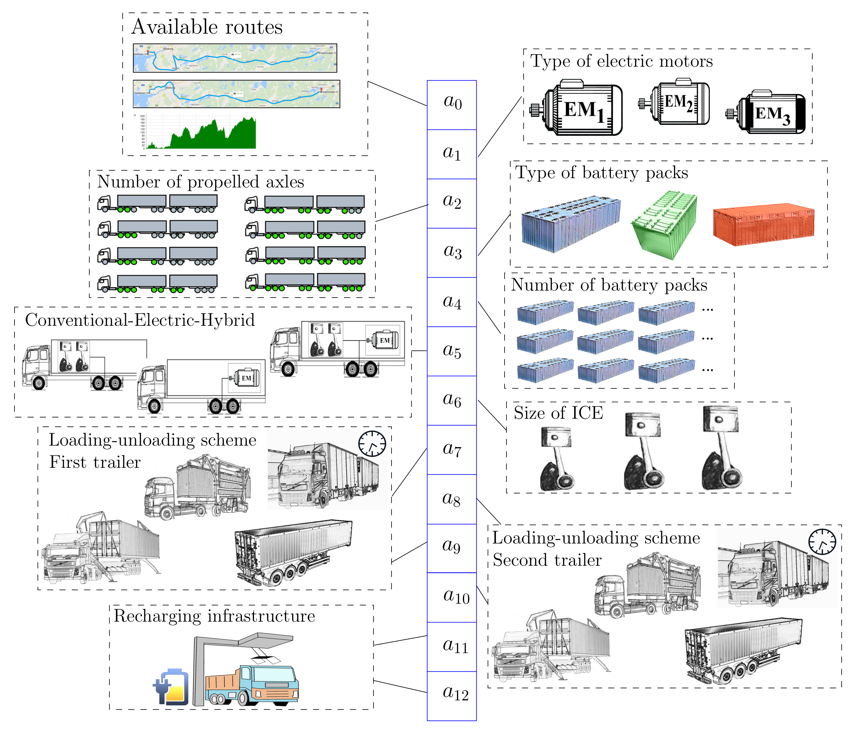
The resulting optimization problem presented in Table 1 is very large, regardless of the size of the transportation network; especially, because there exists many different types of the vehicles. Let us define ${\mathit{X}}_{\mathrm{V}}$ as a set of vehicles containing different vehicle types, and $n_{\mathrm{v}}$ as the total number of vehicle types. An example of ${\mathit{X}}_{\mathrm{V}}$ is depicted in Figure 2. The set of vehicle types ${\mathit{X}}_{\mathrm{V}}$ can be constructed using vehicle design space ${\mathit{S}}_{\mathrm{V}}$. A “design space” is a set containing all design sets of the problem (Figure 3). A “design set” is a set containing all possible choices of a design parameter. A “search space” is a space of optimization design variables. Design space turns to a search space if design sets are treated as ranges of the design variables within an optimization problem.

The vehicle design space, ${\mathit{S}}_{\mathrm{V}}$ can be generalized to a greater extent, thereby covering more aspects of transportation planning and design by not letting design sets ${\mathit{S}}_{\mathrm{V},k}$, $k=1\cdots n_{\mathrm{s}}$ be limited to vehicle-design; but, letting ${\mathit{S}}_{\mathrm{V}}$ to include sets concerning transportation tasks, such as the loading–unloading scheme and recharging infrastructure at each network node, as depicted in Figure 3. Therefore, ${\mathit{X}}_{\mathrm{V}}$ can be defined as an $n_{\mathrm{s}}$-fold Cartesian product, without order, of design sets ${\mathit{S}}_{\mathrm{V},k}$, $k=1\cdots n_{\mathrm{s}}$ belonging to the vehicle design space ${\mathit{S}}_{\mathrm{V}}$. Hereinafter, a bold symbol denotes either a set or a matrix.

$$\begin{array}{cc}\hfill {\mathit{X}}_{\mathrm{V}}=& {\mathit{S}}_{\mathrm{V},1}\times {\mathit{S}}_{\mathrm{V},2}\times \dots \times {\mathit{S}}_{\mathrm{V},n_{\mathrm{s}}}=\hfill \\ \hfill & \{{\mathit{X}}_{\mathrm{V},j}=(a_1,a_2,\dots ,a_{n_{\mathrm{s}}})|a_k\in {\mathit{S}}_{\mathrm{V},k}\in {\mathit{S}}_{\mathrm{V}}\}\hfill \end{array}$$

(1)

where, $j=1,\dots ,n_{\mathrm{v}}$.

A design set (e.g., ${\mathit{S}}_{\mathrm{V},k}$) denotes a set comprising all possible choices of $a_k$. The total number $n_{\mathrm{v}}$ of all possible vehicle types can be calculated as follows.

$$\begin{array}{c}\hfill n_{\mathrm{v}}=\prod _{k=1}^{n_{\mathrm{s}}}{n}_{{\mathit{S}}_{\mathrm{V},k}}\end{array}$$

(2)

In the above equation, $n_{{\mathit{S}}_{\mathrm{V},k}}$ denotes the total number of elements in the design set ${\mathit{S}}_{\mathrm{V},k}$. As can be realized, by increasing $n_{\mathrm{s}}$ and $n_{{\mathit{S}}_{\mathrm{V},k}}$, the number of vehicle types increases quadratically. Moreover, if any of ${\mathit{S}}_{\mathrm{V}k}$s has a continuous range there would exist infinite number of vehicle types, e.g., if the battery size can be selected from a continuous range. The next section presents a method to solve such a problem by redefining and splitting the general optimization problem shown in Table 1 into several optimization subproblems that help determining a close-to-optimum fleet even for large values of $n_{\mathrm{v}}$.

The annual fleet TCO is the sum of the annual TCO of each vehicle of the fleet. The annual TCO of each vehicle, denoted as C, can be expressed as

$$\begin{array}{c}\hfill C=c_{\mathrm{opr}}+c_{\mathrm{dep}}\end{array}$$

(3)

where $c_{\mathrm{dep}}$ indicates the depreciation or yearly cost of investment defined based on the annuity formula (Equation (5)); and $c_{\mathrm{opr}}$ denotes the yearly operational cost given by

$$\begin{array}{c}\hfill c_{\mathrm{opr}}=c_{\mathrm{elec}}+c_{\mathrm{fuel}}+c_{\mathrm{driver}}+c_{\mathrm{maint}}+c_{\mathrm{tax}}+c_{\mathrm{insu}}\end{array}$$

(4)

where variables $c_{\mathrm{elec}}$, $c_{\mathrm{fuel}}$, $c_{\mathrm{driver}}$, $c_{\mathrm{maint}}$, $c_{\mathrm{tax}}$, and $c_{\mathrm{insu}}$, denote annual costs of electricity; fuel; driver labor; vehicle maintenance, including tire, taxes, and insurance, respectively. The annuity formula for calculating depreciation could be defined as

$$\begin{array}{c}\hfill c_{\mathrm{dep}}=[p-\frac{R}{{[1+r]}^{n_{\mathrm{y}}}}]\frac{r}{1-{[1+r]}^{-n_{\mathrm{y}}}}\end{array}$$

(5)

where r denotes the interest or discount rate; $n_{\mathrm{y}}$ denotes the economic life span or planning horizon in years; R denotes the rest value, i.e., the price of a product after completion of its stipulated service life; and p denotes the price of products, such as vehicle hardware or loading, unloading, and recharging infrastructure, when being used for the first time. The price of products can be calculated using the following equation.

$$\begin{array}{c}\hfill p=p_{\mathrm{chass}}+p_{\mathrm{em}}+p_{\mathrm{trans}}+[n_{\mathrm{rep}}+1]p_{\mathrm{batt}}+p_{\mathrm{ice}}+p_{\mathrm{lu}}+p_{\mathrm{rech}}\end{array}$$

(6)

where, $p_{\mathrm{chass}}$ denotes price of the vehicle chassis, such as that of a truck, dolly, or semitrailer, without the associated powertrain and propulsion systems; $p_{\mathrm{em}}$, $p_{\mathrm{trans}}$, $p_{\mathrm{batt}}$, $p_{\mathrm{ice}}$, $p_{\mathrm{lu}}$, and $p_{\mathrm{rech}}$ denote the cost of electric motors, transmission systems, battery packs, internal combustion engine, loading–unloading components, and recharging infrastructure, respectively; and $n_{\mathrm{rep}}$ denotes the number of battery replacements performed during the service life of a vehicle (Equation (A44)), which in this case, has been considered as an investment cost. The battery’s operational life is separated from other vehicle’s component life and it was calculated using vehicle models described in Appendix E according to [48].

It must be noted that $p_{\mathrm{lu}}$ and $p_{\mathrm{rech}}$ are non-linear functions of the number of vehicles since components of the loading–unloading and recharging infrastructure could be shared among many vehicles. Consequently, in Equation (3), C is not a linear function of number of vehicles. For example, a straddle carrier can be shared between many vehicles; whilst an “on-board lift” cannot, refer Figure 4 and Figure 5, according to [11]. Thus, design of the loading–unloading scheme depends on the number of vehicles in the fleet and vice versa. Furthermore, the cost of setting up a charging station is high for a single vehicle; however, when many vehicles use the same station, the per-vehicle cost of charging gets reduced. Thus, infrastructure design is affected by the number of vehicles and vice versa.

The said relations have been observed to affect optimum vehicle design as well. Suppose for a single vehicle, by solving the optimization problem shown in Table 1, it is observed that installation of a large battery pack results in lower cost compared to installing a fast-charging power source. However, sharing of the recharging infrastructure between multiple vehicles makes installation of the fast-charging alternative more feasible compared to installation of the larger battery on each vehicle. This dependence can be eliminated if the infrastructure belongs to a third-party company with a fixed cost of electricity usage. Such a case, however, is not considered in this study.

Constraints of the optimization problem shown in Table 1 are categorized into several groups, each representing a different aspect of the problem. Vehicle dynamic model constraints pertaining to the dynamic, recharging, and powertrain models, inclusive of all equations and inequalities, are described in in Appendix E and inspired by [11,40,49,50,51,52,53,54].

Performance constraints refer to performance-based standards (PBS) that guarantee proper functionality of the vehicles along with on-road safety [55,56,57,58]. In this paper, performance-based standards related exclusively to the longitudinal motion of the vehicle have been considered in terms of gradeability, startability, acceleration, and down-grade holding capability. Gradeability refers to the maximum grade on which a loaded vehicle can maintain forward motion at a certain speed (e.g., 80 km/h). Startability refers to the maximum grade on which a loaded vehicle can start forward motion and travel 10 m in less than 10 s. Acceleration capability denotes time taken by a loaded vehicle to start motion form rest and travel 100 m on a road with zero grade. Finally, down-grade holding capability is defined as the maximum downhill grade on which a loaded vehicle can maintain constant forward speed using auxiliary brakes, such as the engine and/or electric motors. It must be noted that performance-based standards are only affected by vehicle hardware parameters.

Another type of constraints is the one related to transportation tasks and ensures adequate performance of all missions. These constraints, for example, relate to vehicle-loading capacity, pick-up, and delivery during a single trip, the working time, recharging infrastructure powers, and rules prescribed for loading–unloading operations.

Loading–unloading of goods can be performed in four different ways: using an on-board lift (OBL), a straddle carrier (SC) for lifting 20-foot and 40-foot containers, an additional semitrailer (AST) at a node for vehicles with at least one semitrailer, and on-board vehicle waiting (OBW) at a node while all pallets of goods are loaded or unloaded, according to [11].

The selection of a feasible loading–unloading scheme does not include tactical decision variables. Therefore, some rules or constraints need to be set to be able to ensure loading–unloading accessibility and evaluate the corresponding cost. A list of concerned rules is explained in Appendix C and ensures accessibility and feasibility of the loading–unloading scheme.

It should be noted that design of a loading–unloading scheme is coupled with the vehicle-design problem. Having an on-board lift on the vehicle adds to the overall vehicle weight, and thus, energy consumption. Additional semitrailers with propelled axles result in an increase in TCO. Furthermore, the loading–unloading duration time can have an influence on vehicle design to compensate for delays. Loading–unloading schemes could be distinguished in terms of the time required for loading–unloading along with the corresponding investment cost.

4. Method

In this study, it is proposed to split the rather large optimization problem into smaller subproblems or stages. In stage A, a look-up space (i.e., a memory block) of possible best vehicle-infrastructure designs is built by minimizing the unit transportation cost for a given vehicle capacity, mission, and number of vehicles. Here, the vehicle refers to vehicle propulsion hardware, and infrastructure refers to loading–unloading and charging stations positions and powers. In stage B, the look-up space is used in an allocation optimization problem to minimize the fleet TCO, which yields an optimum fleet. The above-defined two stages can be visualized in Figure 6.

The proposed approach for integrated optimization of vehicle-transportation can be used as a solution method for real-world transportation problems involving fleet vehicles powertrain design based on the transportation assignments.

The optimization problem described in Table 1 is rather general, wherein the goal is to determine a group of vehicles with different designs and numbers, the best routes on which they are employed, and corresponding infrastructure. Such a definition helps understanding the complexity of the problem. However, solving such a problem directly might be considered impossible owing to the large number of parameters being sought. The following intuitively obvious postulate was used to split the general optimization problem to several subproblems.

• Postulate: for a given mission, loading capacity, and number of vehicles, there exists only one optimum vehicle type with a corresponding mission infrastructure (i.e., loading–unloading and charging stations) that yields lowest unit transportation cost. It seldom occurs that for a fixed loading capacity, several vehicles with different powertrain designs are found optimum to perform similar tasks. If it happens then any of powertrain designs is equally good and can be selected as an optimum solution.

Using above postulate, the large optimization problem presented in Table 1 can be converted into much smaller $n_{\mathrm{m}}\times n_{\mathrm{lc}}\times N_{\mathrm{v}}$ optimization subproblems, wherein $n_{\mathrm{m}}$ denotes number of missions in set ${\mathit{X}}_{\mathrm{m}}$, which contains all missions, and $n_{\mathrm{lc}}$ denotes number of available loading capacities. The number of vehicles used in the fleet is unknown; moreover, optimum vehicle hardware and infrastructure depend on the number of vehicles employed in a mission; there, therefore, exists a third dimension for number of vehicles $N_{\mathrm{v}}$. To bound values of $N_{\mathrm{v}}$, another set of $n_{\mathrm{m}}\times n_{\mathrm{lc}}$ optimizations must be solved for that is explained in Appendix A.

The suggested solution procedure is as follows.

• Stage A: given a set of missions within the transportation network, a look-up space must be built by determining the best vehicle-infrastructure design for each choice of vehicle capacity, mission, and number of vehicles with that capacity within the mission. The objective function, in this case, includes the unit transportation cost while design variables are inclusive of vehicle hardware, recharging power, and the loading–unloading scheme at each mission node.
• Stage B: the look-up space must be used during allocation optimization, wherein design variables include the number of vehicles and required round-trips to form the optimized fleet, which accomplishes the overall transportation task whilst incurring minimum cost of ownership. Not all vehicles and missions in the look-up space need to be used in the fleet (refer Section 4.2). The objective function, in this case, is fleet TCO.

These above two stages are illustrated in Figure 6, and a detailed explanation is provided in following sections.

A multigraph was used as representative of a transportation network, wherein there may exist several arcs connecting two nodes [59]. Multiple arcs existing between two nodes tend to better reflect real-world transportation scenarios, wherein there may exist several paths between two nodes. Alternatively, additional nodes could be added to the network, where no pickup and delivery could take place. In that case, special care must be spent on excluding these additional nodes from loading–unloading and installation of charging stations decision variables. Using multigraph has been suggested to avoid these extra work. The directed multigraph can be denoted by $G(V,A)$, wherein $V=\{0,1,\dots ,n\}$ represents the set of nodes while A denotes the arc set. Node 0 denotes the depot while $V_{\mathrm{c}}=V\setminus \left\{0\right\}$ denotes n customers. Between each pair of nodes $(q,p)$, $q,p\in V$, there exist $n_{hqp}$ arcs $a_{qpl}$, $a_{qpl}\in h(q,p)$, $l=1,\dots ,n_{hqp}$. Thus, each arc in A, from node q to node p, can be defined as $(q,p,l_{qp})$. Finally, a feasible cyclic route connecting nodes $(0,q_1,q_2,\dots ,q_k,0)$ can be represented by means of a sequence of arcs given by $r=((0,q_1,l_{0q_1}),(q_1,q_2,l_{q_1{q}_2}),\dots ,(q_k,0,l_{q_{k}0}))$. The index set of all feasible routes can be denoted by ${\mathit{X}}_{\mathrm{r}}$; i.e., for all $q\in {\mathit{X}}_{\mathrm{r}}$, $r_q$ is feasible. A feasible route is any cyclic route starting and ending at the depot, passing at least one node. The cyclic route is called a district if the depot is visited several times.

4.1. Stage A: Optimized Vehicle-Infrastructure Design Candidates

The present stage focuses on determining the best vehicle-infrastructure design for each choice of loading capacity and number of vehicles for a given mission, motivated by the postulate above.

After excluding loading capacity from the search space ${\mathit{S}}_{\mathrm{V}}$ or fixing loading capacities to a single value, the optimization problem of stage A, for a given mission i, loading capacity $c_j$, and number of vehicles $N_{\mathrm{v},j}^i$, can be expressed as

$$\begin{array}{c}\hfill \forall i\in \{1,\dots ,n_{\mathrm{m}}\},j\in \{1,\dots ,n_{\mathrm{lc}}\},N_{\mathrm{v},j}^i\in \{1,\dots ,N_{\mathrm{vmax},j}^i\}\end{array}$$

$$\begin{array}{cccc}\hfill & \mathrm{find}\hfill & \hfill & {\mathit{X}}_{\mathrm{rh}}\in {\mathit{X}}_{\mathrm{r}}^i,{\mathit{X}}_{\mathrm{Vl}}\in {\mathit{X}}_{\mathrm{V}}\hfill \\ \hfill & \mathrm{to} \mathrm{minimize}\hfill & \hfill & c_{\mathrm{t}}({\mathit{X}}_{\mathrm{rh}},{\mathit{X}}_{\mathrm{Vl}},c_j,N_{\mathrm{v},j}^i)\hfill \\ \hfill & \mathrm{subject} \mathrm{to}\hfill & \hfill & \hfill \\ \hfill & \hfill & & \mathrm{vehicle}\mathrm{dynamic}\mathrm{model}\mathrm{constraints};\hfill \\ \hfill & \hfill & & \mathrm{performance}\mathrm{constraints};\hfill \\ \hfill & \hfill & & \mathrm{transportation}\mathrm{task}\mathrm{constraints};\hfill \\ \hfill & \hfill & & \mathrm{design}\mathrm{sets}\mathrm{constraints};\hfill \end{array}$$

(7)

where, $c_{\mathrm{t}}$, denotes the annual cost of transporting one unit of freight, which is a nonlinear function of $c_j$ and $N_{\mathrm{v},j}^i$; $c_j$ and $N_{\mathrm{v},j}^i$ denote given inputs representing the loading capacity j and number of vehicles corresponding to that loading capacity in the mission i; ${\mathit{X}}_{\mathrm{r}}^i$ denotes a subset of ${\mathit{X}}_{\mathrm{r}}$, which contains all possible cyclic routes and districts of mission i. It must be noted that, in the optimization problem (7), the design space, depicted in Figure 3, is treated as a search space with fixed vehicle capacity. A new search space ${\mathit{S}}_{\mathrm{RV}}^i$ is defined including ${\mathit{S}}_{\mathrm{V}}$ as well as ${\mathit{X}}_{\mathrm{r}}^i$ marking the range of a design variable—route.

$$\begin{array}{c}\hfill {\mathit{S}}_{\mathrm{RV}}^i=\{{\mathit{X}}_{\mathrm{r}}^i,{\mathit{S}}_{\mathrm{V},1},{\mathit{S}}_{\mathrm{V},2},\dots ,{\mathit{S}}_{\mathrm{V},n_s}\}\end{array}$$

(8)

and

$$\begin{array}{cc}\hfill {\mathit{X}}_{\mathrm{RV}}^i=& {\mathit{X}}_{\mathrm{R}}^i\times {\mathit{S}}_{\mathrm{V},1}\times {\mathit{S}}_{\mathrm{V},2}\times \dots \times {\mathit{S}}_{\mathrm{V},n_s}=\hfill \\ \hfill & \left\{(a_0,a_1,a_2,\dots ,a_{n_{\mathrm{s}}})\right|a_k\in {\mathit{S}}_{\mathrm{RV},k}\in {\mathit{S}}_{\mathrm{RV}}\}\hfill \end{array}$$

(9)

The optimization problem (7) can, therefore, be expressed as

$$\begin{array}{cccc}\hfill & \mathrm{find}\hfill & \hfill & {\mathit{X}}_{\mathrm{RV},l}^i\in {\mathit{X}}_{\mathrm{RV}}^i\hfill \\ \hfill & \mathrm{to} \mathrm{minimize}\hfill & \hfill & c_{\mathrm{t}}({\mathit{X}}_{\mathrm{RV},l}^i,c_j,N_{\mathrm{v},j}^i)\hfill \\ \hfill & \mathrm{subject} \mathrm{to}\hfill & \hfill & \mathrm{all}\mathrm{constraints};\hfill \end{array}$$

(10)

or reformulated as follows using design variables $a_k$.

$$\begin{array}{cccc}\hfill & \mathrm{find}\hfill & \hfill & a_k\in {\mathit{S}}_{\mathrm{RV},k}^i\in {\mathit{S}}_{\mathrm{RV}}^i,k=0,\dots ,n_{\mathrm{s}}\hfill \\ \hfill & \mathrm{to} \mathrm{minimize}\hfill & \hfill & c_{\mathrm{t}}(a_0,a_1,\dots ,a_{n_{\mathrm{s}}},c_j,N_{\mathrm{v},j}^i)\hfill \\ \hfill & \mathrm{subject} \mathrm{to}\hfill & \hfill & \mathrm{all}\mathrm{constraints}.\hfill \end{array}$$

(11)

The optimization problem of the form described in (11), where $a_k$ serve as optimization design variables in the $n_{\mathrm{s}}+1$ dimensional space ${\mathit{S}}_{\mathrm{RV}}^i$, of the range specified by ${\mathit{S}}_{\mathrm{RV},k}^i$, could be solved using a stochastic optimization technique, such as particle swarm optimization (PSO) [60,61], and according to the algorithm described in [62]. PSO demonstrates good performance when dealing with non-smooth and non-convex problems. However, it is not very efficient at handling design variables exceeding 30 in number. Ref. [61] provided a comprehensive comparison of different methods. Moreover, the optimization problem must be solved for a number of times to reduce the probability of obtaining a solution far from the global optimum. In the presented case-study, many runs resulted in a similar solution referred as an local optimum solution where, considering the fact that each run was initialized with different initial points (i.e., population), there is a high probability that the obtained solution is a global optimum.

Owing to the inherent nonlinearity and coupling between the number of vehicles, with different payload capacities on a mission, and their corresponding hardware setup, the optimization problem (11) must be solved for all possible numbers of vehicles, i.e., for $N_{\mathrm{v},j}^i=1,\dots ,N_{\mathrm{vmax},j}^i$. $N_{\mathrm{vmax},j}^i$, in this case, denotes the maximum number of vehicles, of the same capacity $c_j$, which must be used in a given mission i.

To determine the lower bound for $N_{\mathrm{vmax},j}^i$, a corresponding optimization problem must be solved to also determine optimum values of masses $m_{\mathrm{L},j}^i$ and $m_{\mathrm{U},j}^i$ of the loaded and unloaded freight, respectively, by means of a vehicle performing identical trips within a mission. By having a single vehicle performing $n_{\mathrm{t}}$ identical trips or employing $n_{\mathrm{t}}$ identical vehicles, each performing a single trip, the total transportation demand of the mission can be satisfied. It should be noted that each vehicle of the same type performs identical trip(s) within a mission. The optimization problem used for finding $N_{\mathrm{vmax},j}^i$, $m_{\mathrm{L},j}^i$ and $m_{\mathrm{U},j}^i$ is described in Appendix A.

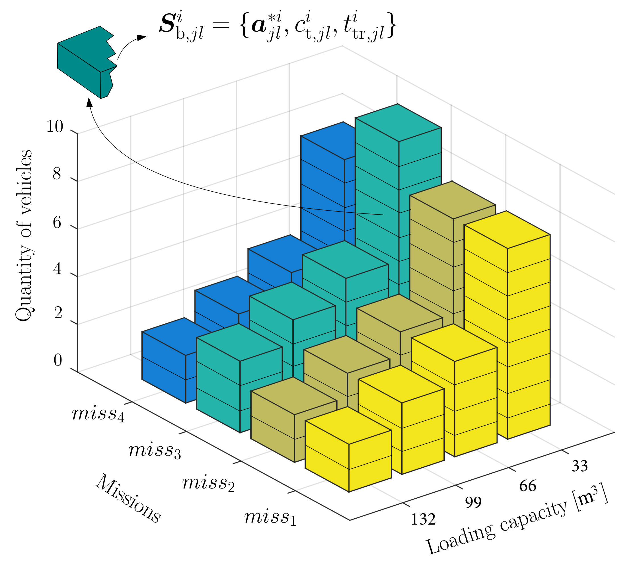
After solving optimization problem described in (11) for all missions $i=1,\dots ,n_{\mathrm{m}}$, loading capacities $j=1,\dots ,n_{\mathrm{lc}}$, and quantity of vehicles $N_{\mathrm{v},j}^i=1,\dots ,N_{\mathrm{vmax},j}^i$, corresponding solutions obtained must be stored and used as the look-up space ${\mathit{S}}_{\mathrm{b}}$ in stage B. An example of such a space is depicted in Figure 7. The stored information in the look-up space corresponds to ${\mathit{a}}^{*}=(a_0^{*},\dots a_{n_{\mathrm{s}}}^{*})$, $c_{\mathrm{t}}$, and $t_{\mathrm{tr}}$, i.e., optimized design, the unit transportation cost, and trip duration time, respectively; that is

$$\begin{array}{c}\hfill {\mathit{S}}_{\mathrm{b},jl}^i=\{{\mathit{a}}_{jl}^{*i},c_{\mathrm{t},jl}^i,t_{\mathrm{tr},jl}^i\},\forall i\in \{1,\dots ,n_{\mathrm{m}}\},j\in \{1,\dots ,n_{\mathrm{lc}}\},l\in \{1,\dots ,N_{\mathrm{vmax},j}^i\}\end{array}$$

(12)

4.1.1. Unit Yearly Transportation Cost

The total annual cost of a heavy combination vehicle per unit freight transported, denoted as $c_{\mathrm{t}}$, for a given mission can be expressed as

$$\begin{array}{c}\hfill c_{\mathrm{t}}(a_0,\dots ,a_{n_{\mathrm{s}}},c,N_{\mathrm{v}})=\frac{C(a_0,\dots ,a_{n_{\mathrm{s}}},c,N_{\mathrm{v}})}{f_{\mathrm{tr}}}\end{array}$$

(13)

where, c denotes the loading capacity, $f_{\mathrm{tr}}$ indicates the number of freight units transported in a year from/to a depot, and C represents TCO given by Equation (3).

Following Equations (3) and (4), operational costs could be calculated as follows.

$$\begin{array}{cc}\hfill & c_{\mathrm{fuel}}=p_{\mathrm{f}}{F}_{\mathrm{c}}{N}_{\mathrm{tf}}{n}_{\mathrm{d}}{N}_{\mathrm{v}}\hfill \\ & c_{\mathrm{elec}}=p_{\mathrm{el}}{E}_{\mathrm{el}}{N}_{\mathrm{tf}}{n}_{\mathrm{d}}{N}_{\mathrm{v}}\hfill \\ & c_{\mathrm{driver}}=p_{\mathrm{d}}{t}_{\mathrm{tr}}{N}_{\mathrm{tf}}{n}_{\mathrm{d}}{N}_{\mathrm{v}}\hfill \\ & c_{\mathrm{maint}}=c_{\mathrm{m}}[c_{\mathrm{fuel}}+c_{\mathrm{elec}}]N_{\mathrm{v}}\hfill \end{array}$$

(14)

where $p_{\mathrm{f}}$, $p_{\mathrm{el}}$, $n_{\mathrm{d}}$, and $p_{\mathrm{d}}$ denote prices of diesel fuel, electricity, number of working days per year, and driver salary, respectively. $F_{\mathrm{c}}$ denotes fuel consumed during a trip (Equation (A23)), $E_{\mathrm{el}}$ denotes electricity consumed during a trip (Equation (A32)), $c_{\mathrm{m}}$ is a constant, which provides a rough estimate of maintenance costs as a fraction of the energy cost; $t_{\mathrm{tr}}$ denotes trip time, which can be calculated using the vehicle dynamic model (Equation (A42)). $N_{\mathrm{tf}}$ denotes the maximum number of trips a fully operational vehicle performs per day, and can be expressed as

$$\begin{array}{c}\hfill N_{\mathrm{tf}}=\lfloor \frac{w_{\mathrm{tmax}}}{t_{\mathrm{tr}}}\rfloor \end{array}$$

(15)

where, $w_{\mathrm{tmax}}$ denotes the maximum allowable working time per day. The operator $\lfloor a\rfloor$ provides the closet integer equal to or less than a.

Description of a vehicle dynamic model along with the procedure for calculating values of $F_{\mathrm{c}}$, $E_{\mathrm{el}}$, and $t_{\mathrm{tr}}$ is given in Appendix E according to [48], and all parameters and prices are included in the Appendix F.

Moreover, the cost of loading-unloading equipments $p_{\mathrm{lu}}$ and charging infrastructure $p_{\mathrm{rech}}$ for each vehicle in mission i are given by

$$\begin{array}{c}\hfill p_{\mathrm{lu}}=\sum _{k\in {\mathit{I}}_{\mathrm{n}}^i}\frac{p_{\mathrm{LU},k}}{N_{\mathrm{v}}},p_{\mathrm{rech}}=\sum _{k\in {\mathit{I}}_{\mathrm{n}}^i}\frac{p_{\mathrm{CH},k}}{N_{\mathrm{v}}}\end{array}$$

(16)

where ${\mathit{I}}_{\mathrm{n}}^i$ is a set containing node indices of the ith mission, $p_{\mathrm{LU},k}$ and $p_{\mathrm{CH},k}$ denotes the cost of shared loading–unloading equipments and charging infrastructure at node k, respectively.

4.1.2. Optimization-Problem Constraints

Constraints of the optimization problem (11) include vehicle-model constraints pertaining to the dynamic, recharging, and powertrain models, inclusive of all equations and inequalities, together with a battery degradation model are described in Appendix E according to [48], inspired by [11,49,50,51,52,53,54].

Performance constraints, i.e., gradeability $G_{\mathrm{r}}$, startability $S_{\mathrm{r}}$, acceleration capability $A_{\mathrm{c}}$, and down-grade holding capability $D_{\mathrm{g}}$ could be summarized in the mathematical form as follows.

$$\begin{array}{c}{G}_{\mathrm{r}}(a_1,\dots ,a_{n_{\mathrm{s}}})\ge G_{r,min}\hfill \\ S_{\mathrm{r}}(a_1,\dots ,a_{n_{\mathrm{s}}})\ge S_{r,min}\hfill \\ A_{\mathrm{c}}(a_1,\dots ,a_{n_{\mathrm{s}}})\le A_{c,max}\\ D_{\mathrm{g}}(a_1,\dots ,a_{n_{\mathrm{s}}})\ge D_{g,min}\end{array}$$

(17)

It must be noted that the performance constraints are only affected by vehicle hardware design parameters. Refer Appendix F for selected values of the performance constraints.

Part of transportation constraints must be covered under the optimization problem in stage B (refer Section 4.2). Other constraints that must be considered in the optimization problem (11) relate to vehicle-loading capacity, pick-up, and delivery during a single trip, as described in Appendix A by Equations (A2)–(A8), as well as the working time, given by Equation (A42). Another set of transportation-task constraints pertaining to rules prescribed for loading–unloading operations are explained in Appendix C. No mathematical description about loading–unloading operations is provided in this paper to avoid notational complexity.

4.2. Stage B: The Optimized Fleet

By solving the optimization problem (11) for all available mission choices, loading capacities, and number of vehicles, a set or a space ${\mathit{S}}_{\mathrm{b}}$ containing optimum design candidates is obtained. Candidate designs belonging to this space must be optimally allocated by deciding which designs must work together to satisfy the required pick-up and delivery demands of the transportation network. Fleet composition and sizing is finalized in this stage; moreover, the total number of trips to be performed by each vehicle type is also finalized. Minimum value of the total cost of fleet ownership can be realized by solving the following optimization problem.

$$\begin{gathered} \begin{array}{ccc}\mathrm{find}\hfill & & {\mathit{N}}_{\mathrm{v}}\in {\mathbb{N}}^{n_{\mathrm{m}}\times n_{\mathrm{lc}}},{\mathit{N}}_{\mathrm{t}}\in {\mathbb{N}}^{n_{\mathrm{m}}\times n_{\mathrm{lc}}}\hfill \\ \mathrm{to} \mathrm{minimize}\hfill & & C({\mathit{N}}_{\mathrm{v}},{\mathit{N}}_{\mathrm{t}})=n_{\mathrm{d}}{\displaystyle \sum _{i=1}^{n_{\mathrm{m}}}}{\displaystyle \sum _{j=1}^{n_{\mathrm{lc}}}}[N_{\mathrm{vf},j}^i{N}_{\mathrm{tf},j}^i{c}_j{c}_{\mathrm{t},jl}^i+ \\ \hspace{1em}\hspace{1em}\hspace{1em}{N}_{vp,j}^i{N}_{\mathrm{tp},j}^i{c}_j{c}_{\mathrm{t},j}^i({\mathit{a}}_{jl}^i,c_j,N_{\mathrm{vp},j}^i)]\hfill \\ \mathrm{subject} \mathrm{to}\hfill & \hfill & \hfill \end{array} \end{gathered}$$

(18)

$$\begin{array}{c}{N}_{\mathrm{tf},j}^i=\lfloor \frac{w_{\mathrm{tmax}}^i}{t_{\mathrm{tr},jl}^i}\rfloor \hfill \end{array}$$

(19)

$$\begin{array}{c}{N}_{\mathrm{vf},j}^i=\lfloor \frac{N_{\mathrm{t},j}^i}{N_{\mathrm{tf},j}^i}\rfloor \hfill \end{array}$$

(20)

$$\begin{array}{c}{N}_{\mathrm{tp},j}^i=N_{\mathrm{t},j}^i-N_{\mathrm{tf},j}^i{N}_{\mathrm{vf},j}^i\hfill \end{array}$$

(21)

$$\begin{array}{c}{N}_{\mathrm{vp},j}^i=N_{\mathrm{v},j}^i-N_{\mathrm{vf},j}^i\hfill \\ c_{\mathrm{t},j}^i({\mathit{a}}_{jl}^i,c_j,N_{\mathrm{vp},j}^i)=\hfill \end{array}$$

(22)

$$\begin{array}{c}\frac{c_{\mathrm{opr}}({\mathit{a}}_{jl}^i,c_j,N_{\mathrm{vp},j}^i)+c_{\mathrm{dep}}({\mathit{a}}_{jl}^i,c_j,N_{\mathrm{vp},j}^i)}{f_{\mathrm{tr}}({\mathit{a}}_{jl}^i,c_j,N_{\mathrm{vp},j}^i)}\hfill \end{array}$$

(23)

$$\begin{array}{c}\{{\mathit{a}}_{jl}^i,c_{\mathrm{t},jl}^i,t_{\mathrm{tr},jl}^i\}={\mathit{S}}_{\mathrm{b},jl}^i,l=N_{\mathrm{v},j}^i\hfill \end{array}$$

(24)

$$\begin{array}{c}{N}_{\mathrm{v},j}^i{N}_{\mathrm{tf},j}^i\ge N_{\mathrm{t},j}^i\forall i\in {\mathit{X}}_{\mathrm{m}},j=1\dots n_{\mathrm{lc}}\hfill \end{array}$$

(25)

$$\begin{array}{c}{\displaystyle \sum _{i=1}^{n_{\mathrm{m}}}}{\displaystyle \sum _{j=1}^{n_{\mathrm{lc}}}}{N}_{\mathrm{t},j}^i{m}_{\mathrm{L},jk}^i\ge Q_{\mathrm{p},k},\forall k\in V\hfill \end{array}$$

(26)

$$\begin{array}{c}{\displaystyle \sum _{i=1}^{n_{\mathrm{m}}}}{\displaystyle \sum _{j=1}^{n_{\mathrm{lc}}}}{N}_{\mathrm{t},j}^i{m}_{\mathrm{U},jk}^i\ge Q_{\mathrm{d},k},\forall k\in V\hfill \end{array}$$

(27)

where ${\mathit{N}}_{\mathrm{v}}$ is a matrix containing the number of vehicles with different loading capacities employed in different missions; ${\mathit{N}}_{\mathrm{t}}$ refers to a matrix containing the total number of round trips per day that ${\mathit{N}}_{\mathrm{v}}$ vehicles perform together; $N_{\mathrm{t},j}^i$ corresponds to the total number of identical trips that must be performed by all vehicles with loading capacity $c_j$ in the ith mission; $N_{\mathrm{v},j}^i$ corresponds to the total number of vehicles with loading capacity $c_j$ in the ith mission; $n_{\mathrm{m}}$ denotes the total number of missions constituting the set ${\mathit{X}}_{\mathrm{m}}$; $n_{\mathrm{lc}}$ corresponds to the total number of loading-capacity choices. The objective function C corresponds to the total cost of fleet ownership per year represented as [€/year]. Subscripts f and p translate to fully operational and partially operational, respectively; and $n_{\mathrm{d}}$ is the number of working days per year. Fully-operational vehicles perform the maximum number of trips $N_{\mathrm{tf},j}^i$ per day before maximum limit of daily working hours $w_{\mathrm{tmax}}^i$ is violated. Having a flexible maximum limit daily working hours is shortly discussed later in discussion section. A vehicle performing any number of trips less than $N_{\mathrm{tf},j}^i$ is referred to as being partially operational. Constraints (19)–(22) yield the number of fully and partially operated vehicles—$N_{\mathrm{vf},j}^i$ and $N_{\mathrm{vp},j}^i$ along with the maximum number of trips per day $N_{\mathrm{tf},j}^i$ as well as number of trips $N_{\mathrm{tp},j}^i$ less than maximum.

While building the look-up space ${\mathit{S}}_{\mathrm{b}}$ by solving the optimization problem (11), it was assumed that all vehicles are fully operational, i.e., all vehicles perform maximum number of trips per day, by evaluating Equation (13) using Equation (15). We made this assumption to avoid complication of adding a fourth dimension to the look-up space, since most of the fleet vehicles perform the maximum number of trips. If, for some reason, a fully operational vehicle is not required, it must be redesigned for the given required number of trips per day. Any redesigning of vehicles is not considered in this paper, and partially operational vehicles are considered to have a design similar to that of fully operational. For such vehicles, however, the annual ownership cost per unit freight, as described in Equation (13), must be re-evaluated for the assigned number of trips the vehicle performs per day. This implies replacing $N_{\mathrm{tf},j}^i$ by $N_{\mathrm{tp},j}^i$ in Equation (14). This constraint is expressed by Equation (23) , wherein ${\mathit{a}}_{jl}^i$ represents the vehicle-infrastructure design; values of ${\mathit{a}}_{jl}^i$, $c_{\mathrm{t},jl}^i$, and $t_{\mathrm{tr},jl}^i$ are adopted from the look-up space expressed by the constraint (24). The reason why ${\mathit{N}}_{\mathrm{v}}$ is considered as an optimization variable is that it cannot directly be calculated from ${\mathit{N}}_{\mathrm{t}}$, since vehicle-infrastructure design and correspondingly, the maximum number of trips per day or trip duration time remains unknown if one does not know which block to choose corresponding to the number of vehicles in the look-up space.

The constraint described in (25) ensures that the daily working time is not violated as well as that the selected total number of trips are performed by the selected number of vehicles. Constraints described in (26) and (27) guarantee that the daily demands concerning pick-up and delivery of all nodes of the transportation network are met. In this case, V denotes the set of all nodes in the transportation network and $m_{\mathrm{L}}$ and $m_{\mathrm{U}}$ denote masses of the loaded and unloaded freight during a trip, respectively, obtained by solving the optimization problem described by (A1)–(A8) in Appendix A, $Q_{\mathrm{p},k}$ denotes individual units (for example mass) of the total daily demand of freight pick-up from node k and $Q_{\mathrm{d},k}$ represents units of the total freight that needs to be delivered to node k.

Vehicle missions within transportation networks may overlap. Constraints above ensure that the entire transportation task of the network is performed via all or some missions within the specified daily working time window. The optimization problem (18)–(27) can also be solved using the PSO method.

The search space within the optimization problem (18)–(27) comprises two 3D spaces, as depicted in Figure 8. The range of design variables is described by the third dimension of space—the number of vehicles and total number of round trips. Both these ranges have the same size starting from zero to a maximum number given by Equations (A1)–(A8).

5. Case Study: Auto-Freight Project

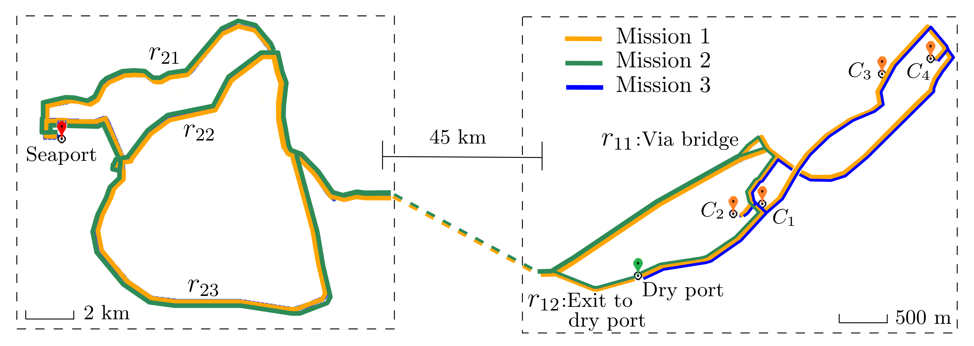
The case-study problem considered in this study relates to a project called Highly Automated Freight Transports funded by Vinnova (Ref number 2016-05413 and 2016-05415) in Sweden. This project was initiated to design and manage transportation of goods in containers between Gothenburg seaport and city Borås. Here, we investigate a scenario considering a dry port, close to Borås, where goods must be loaded/unloaded onto/from transport vehicles and subsequently transported to local companies.

A dry port is an inland terminal, where goods can be picked-up from or delivered to in a manner similar to a seaport [63,64]. Benefits offered by a dry port include the possibility of switching over to more efficient especially developed transportation solutions and logistic convenience. Road connections for such a transportation network are depicted in Figure 9, wherein $r_{kl}$ represents different road sections and $C_i$ denotes the ith customer. The routes within the mission are described in Appendix D. To evaluate the fuel consumption, each cyclic route is described by an operating cycle according to Appendix E.

Requests for pick-up and delivery of goods at each node are listed in

Table 2. Constant daily pick-up and delivery requests.

	${\mathit{C}}_1$	${\mathit{C}}_2$	${\mathit{C}}_3$	${\mathit{C}}_4$	Dryport	Seaport
Delivery [ton/day], [33-m${}^3$ container/day], [${\mathrm{m}}^3$/day]	24, 4, 113	12, 2, 57	12, 2, 57	0	48, 8, 226	28, 4, 132
Pick-up [ton/day], [33-m${}^3$ container/day], [${\mathrm{m}}^3$/day]	0	0	0	28, 4, 132	48, 8, 226	48, 8, 226

. Goods could be delivered or picked-up in sets of 500-kg pallets, 20-foot, or 40-foot containers. Duration of the normal working time per day was set as 600 min, including minimum 90 min of waiting time at the seaport during each visit. Longer working times were allowed up to 960 min, with extra penalty, however, on operational costs. There were 220 working days per year within an 8-year service life of a vehicle. Total distance covered in a round trip measured approximately 140 km, the exact value varying depending on the route selection. Other mission data related to economics and transportation design could be found in Appendix F. 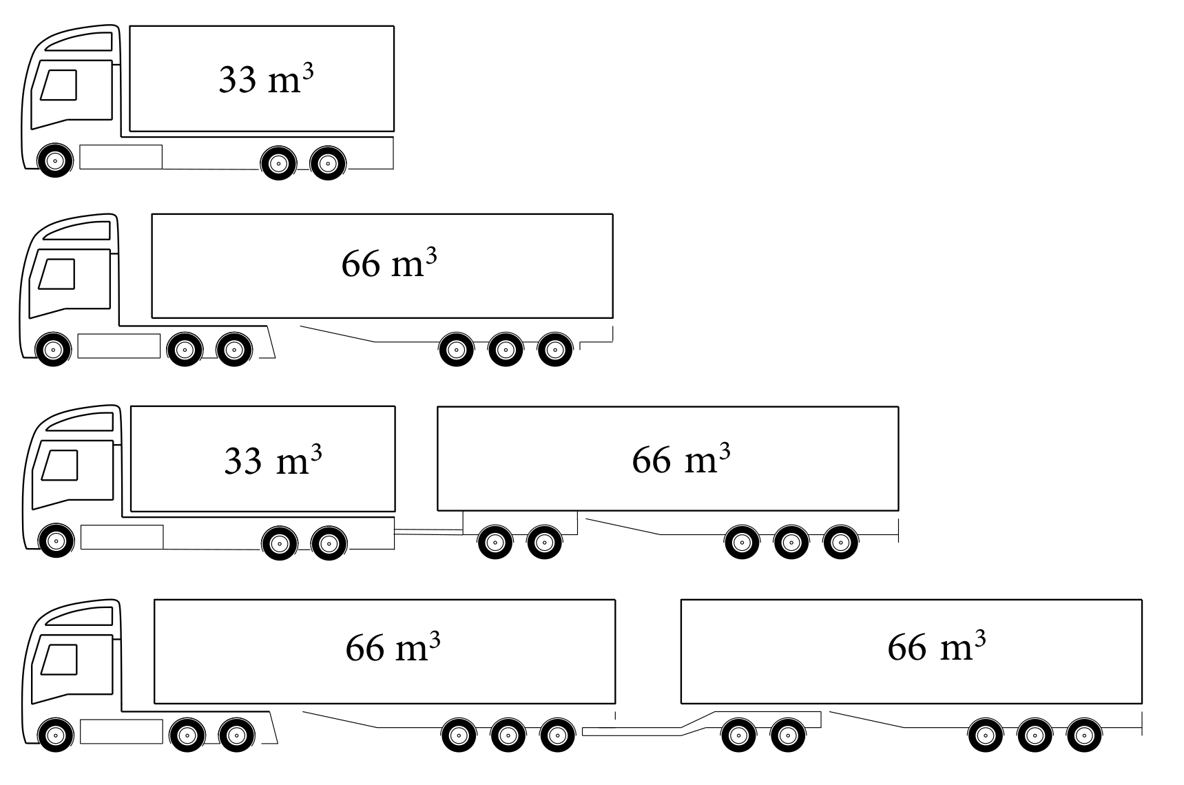The optimization problem shown in Table 1 was solved for the above case study. The range of the mission design variable included three missions shown in Figure 9. The range of vehicle sizes are depicted in Figure 10. The charging power at each node ranged between 0 and 180 kW. Zero-charging power means that there is no charging station at the node, therefore, the solution of the optimization problem also defined the location of the charging stations. Furthermore, the range of loading–unloading design variable, at each of the nodes and for each of the semitrailers of the vehicles, included four loading–unloading schemes (i.e., OBL, SC, AST, and OBW) together with no-loading–unloading (NLU), meaning that no action should be done at the node regarding loading–unloading for the corresponding container. Vehicle types were defined using the design space given by Equation (A9), that together with possibility of having on-board lift resulted in about 83,000 different vehicle types, despite the small size of the vehicle design sets. Please refer to Appendix B for the description about the ranges of the vehicle design sets.

5.1. Presenting the Solution

For the case study problem presented above, stages A and B were solved and the solutions were compared among 20 and 100 runs, respectively, where about 60% of solutions were found to be similar.

The solution yields the optimum vehicle fleet given the set of routes/missions shown in Figure 9. Figure 11 depicts the optimization result for the case-study problem presented above with a maximum daily working time of 10 h and daily demand flow of 226 cubic meters. The optimum fleet includes one vehicle combination comprising one tractor, one dolly, and two semitrailers with a total loading capacity of 132 m${}^3$ and performing two trips per day on the second mission; one vehicle combination comprising one tractor and one semitrailer with a loading capacity of 66 m${}^3$ and making four trips per day on the third mission whilst also comprising three straddle carriers, an additional semitrailer, and two charging stations. Specifications pertaining to vehicle and recharging power are provided in

Table 3. Vehicle-hardware, loading–unloading (LU) scheme, and recharging-power designs of three selected optimized vehicles on three missions with the number of vehicles being one on a mission. ${\mathit{X}}_{\mathrm{r}}^i$ denotes mission i, that contains different choices of the cyclic routes within mission explained in Appendix D. EM denotes electric motor; please refer to Appendix F for EMs specification.

	Mission 1, (${\mathit{X}}_{\mathit{r}}^1$)	Mission 2, (${\mathit{X}}_{\mathit{r}}^2$)	Mission 3, (${\mathit{X}}_{\mathit{r}}^3$)
Maximum working time per day (h)	16	10	10
Route	${\mathit{X}}_{\mathrm{r}}^1\left(1\right)$	${\mathit{X}}_{\mathrm{r}}^2\left(1\right)$	${\mathit{X}}_{\mathrm{r}}^3\left(1\right)$
Conventional-Electric-Hybrid	Electric	Electric	Electric
Loading capacity (m${}^3$)	132	132	66
Type of electric motor	EM2	EM2	EM1
Number of electric motors	6	6	4
Total number of battery packs	13	12	3
Total size of battery packs (kWh)	438.75	405	101.25
Total mass of battery packs (ton)	3.25	3	0.75
Size of IC engine (lit)	-	-	-
Recharging at Dryport (kW)	10	10	10
Recharging at Seaport (kW)	70	70	-
LU at Dryport, 1st semitrailer	SC	SC	SC
LU at Dryport, 2nd semitrailer	SC	SC	-
LU at Seaport, 1st semitrailer	SC	SC	-
LU at Seaport, 2nd semitrailer	SC	SC	-
LU at C1, 1st semitrailer	NLU	-	SC
LU at C1, 2nd semitrailer	AST	-	-
LU at C2, 1st semitrailer	NLU	-	OBW
LU at C2, 2nd semitrailer	OBW	-	-
LU at C3, 1st semitrailer	NLU	-	OBW
LU at C3, 2nd semitrailer	OBW	-	-
LU at C4, 1st semitrailer	NLU	-	AST
LU at C4, 2nd semitrailer	AST	-	-

. All containers measured 33 m${}^3$ volume.

Figure 12 depicts the optimum fleet for two different maximum daily working durations—10 h and 16 h—and demands of daily freight flow—48 and 168 tons—corresponding to 226 and 792 m${}^3$, respectively. A small container has a loading capacity of 33 m${}^3$ or 7 tons of intended freight. Figures demonstrate that the optimum fleet is very sensitive to optimization-problem constraints—daily flow and maximum daily working hours. Selection of different constraints, other than ones shown in Figure 12, might result in a different optimum-fleet configuration.

Designs of vehicle hardware, loading–unloading schemes, and recharging power for the three optimized vehicles selected for the three missions are listed in Table 3 while the number of vehicles is assumed to be one on a mission.

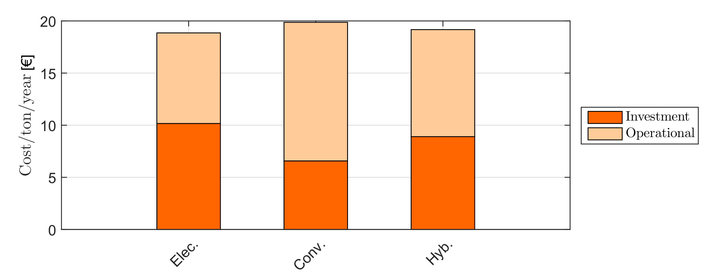
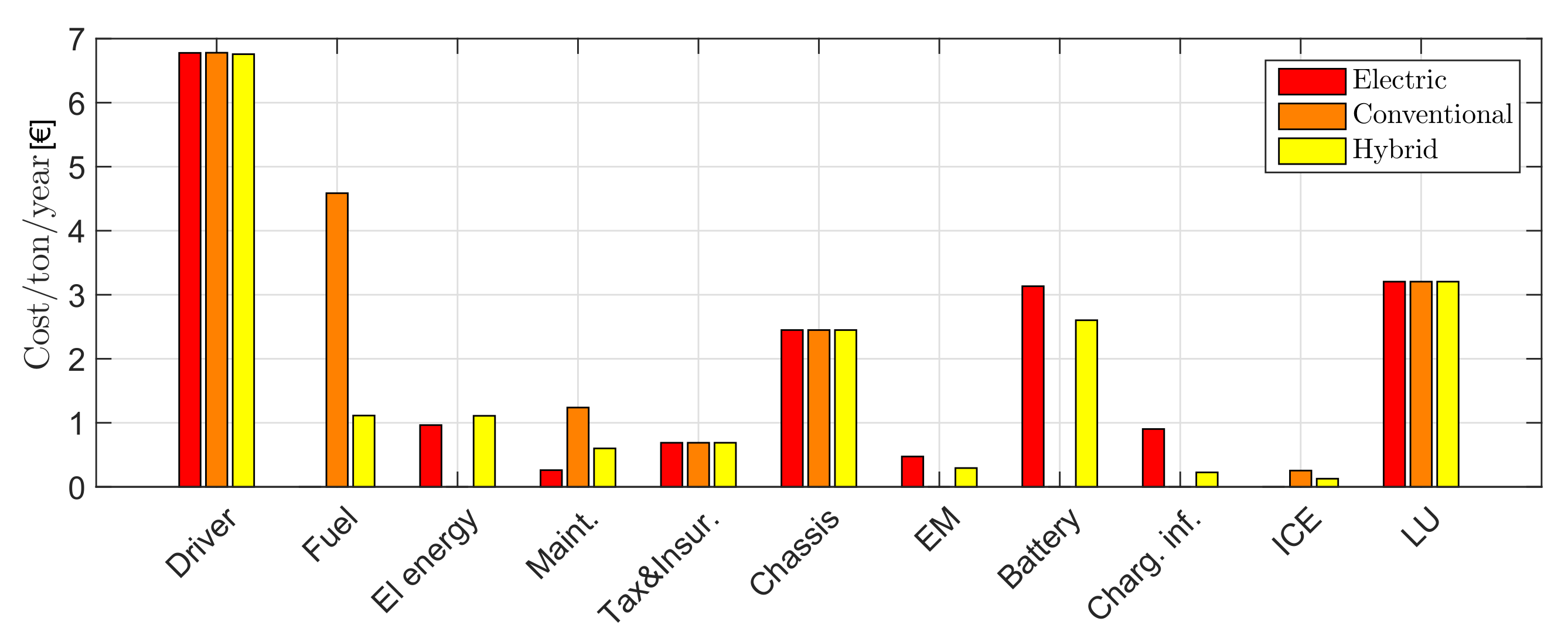
Figure 13 and Figure 14 compare annual costs incurred per unit freight transported by optimum conventional, fully electric, and plug-in hybrid vehicles with a loading capacity of 132 m${}^3$ during the first mission. Data depicted in Figure 13 and Figure 14 were obtained by solving optimization problem shown in Table 1 with the powertrain fixed as being either of the conventional, fully electric, or hybrid type. It can be observed that use of the fully-electric vehicle demonstrated a lower TCO per year compared to using conventional and hybrid vehicles. Moreover, the operational cost of the conventional vehicle is seen to be high due to fuel consumption. On the other hand, the investment cost of the battery-electric and hybrid vehicles is high due to the high battery cost. However, hybrid vehicles offer benefits of good energy-management strategy, which in turn, reduces operational costs. The control strategy here for optimizing the powertrain is ruled-based, which is similar to the instantaneous optimization reported by [49]. Through the use of an optimum energy-management strategy, overall energy costs could be reduced by up to 4% when moving in traffic with a smooth variation in speed on the roads considered in this study.

To investigate the sensitivity of annual costs incurred per unit freight with regards to variation in design parameters, an electric vehicle on the first mission was selected with a fixed design; subsequently, the value of only one parameter was changed within the admissible range. The corresponding result is depicted in Figure 15 and Figure 16. It must be noted that most of the observations and conclusions drawn here about design and performance of electric heavy-vehicles are general and not limited to the case study.

The dependence of mission costs on road conditions can be rather high, if the concerned vehicle fails to complete the trip on time or vehicle hardware is not feasible to operate on the given road. However, the vehicle selected for sensitivity analysis was both feasible and could make the trip on time under all road conditions. Thus, the only sources of incurring extra costs on different roads were the driver and energy costs, in view of the increased trip duration and distance, as depicted on the top-left of Figure 15.

There exists a linear relationship between the TCO and number of electric motors until 10 electric motors are installed in a vehicle. As can be observed in the middle left of Figure 15, a jump in total cost is observed when 11 electric motors are used in a vehicle. The reason behind this jump is the observed increase in loading–unloading costs, because the 11th electric motor must be placed on the last semitrailer. The total loading–unloading cost, therefore, increases if additional semitrailers with propelled axles are assigned to the mission.

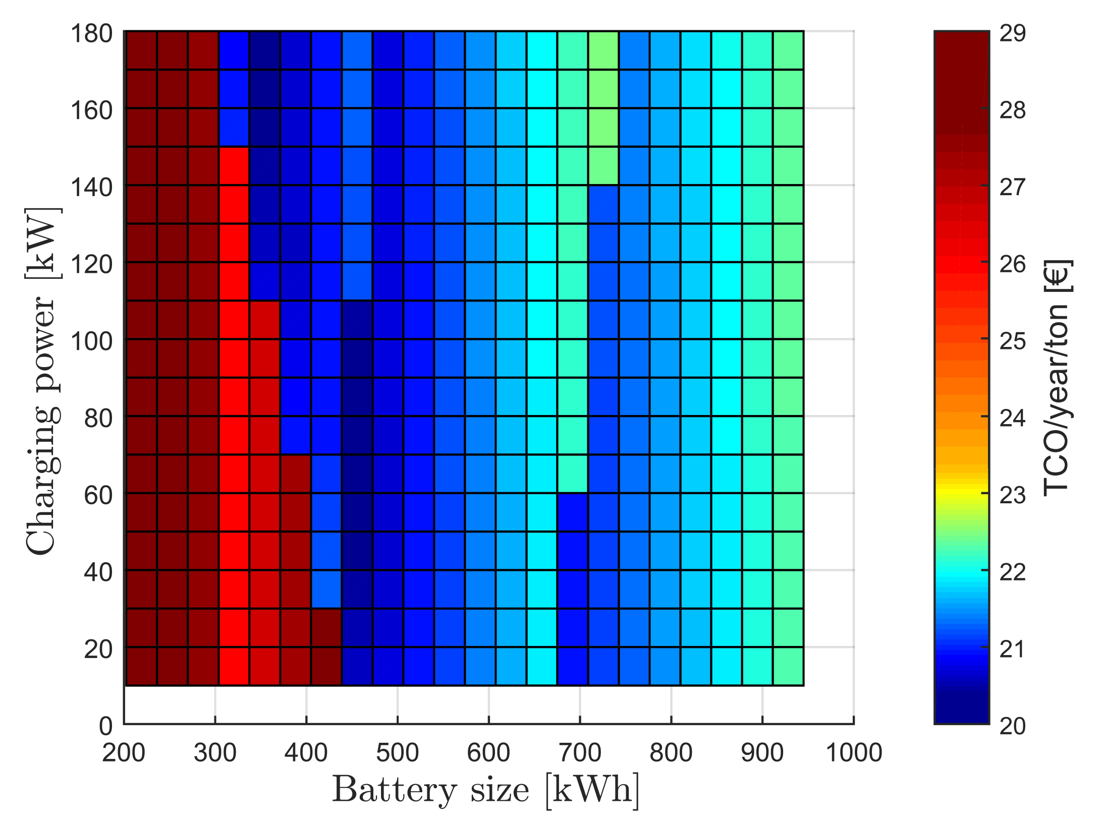
The TCO per ton of freight demonstrated a linear trend with respect to the recharging power as long as no battery replacement was required. Battery degradation increases with large recharging power and small battery size; thus, batteries of a given size and capacity tend to exhaust earlier, if the recharging power is increased. Figure 17 illustrates this behavior. Trade-offs between fast and slow charging have already been discussed by [30] among others in the literature.

As can be observed, the TCO is greatly influenced by battery size and charging power, thereby producing several local minima. Battery size influences the total operational time in terms of the optimum recharging time, as well as power needed to fully charge the batteries, thereby facilitating fully electric vehicles to reach the next charging station. Additionally, vehicle speed can also be affected by the maximum available battery power. Moreover, batteries of different sizes possess different lifetimes. Together, all these factors cause a large variation in TCO with respect to battery size, as depicted in Figure 15 and Figure 17. The reason behind having a large drop in most of cost indicators for battery sizes larger than a threshold is that the vehicle could perform one more trip within the given daily time window as the result of higher power availability, thereby increasing the freight transported per day and consequently reducing the annual unit transportation cost. A drop in cost is, therefore, observed corresponding to all cost indicators in the middle-right of Figure 15, except for the driver cost, the reason being that driving time increases accordingly (within the time window) and also there is an increase in waiting time at a charging station in order to charge the batteries sufficiently so that the final trip could be performed. Furthermore, in the same figure, each drop in battery cost with increase in battery size implies that one less battery replacement is needed during the service life of a vehicle.

Further, the optimum battery size as well as recharging power can be affected by the number of vehicles employed during a mission. As previously discussed, investment cost per vehicle reduces via sharing of charging stations; it is, therefore, favorable to have a large recharging power compared to large battery size.

Table 4. Two optimum types of electric vehicles assigned to mission ${\mathit{X}}_{\mathrm{r}}^1$ for fully loaded vehicles and two trips per day.

Optimized for	${\mathit{type}}_{\mathbf{em}}$	${\mathit{N}}_{\mathbf{em}}$	${\mathit{N}}_{\mathbf{pack}}$	${\mathit{RC}}_1$ (kW)	${\mathit{RC}}_2$ (kW)	Cost, if One Vehicle in the Mission ($\frac{€}{\mathbf{ton}·\mathbf{year}}$)	Cost, if Two Vehicles in the Mission ($\frac{€}{\mathbf{ton}·\mathbf{year}}$)
one vehicle in the mission	$E{M}_2$	6	14	10	90	15.48	13.63
two vehicles in the mission	$E{M}_2$	6	9	100	130	15.65	13.38

lists hardware setups and recharging powers for two optimum fully electric vehicles assigned to mission ${\mathit{X}}_{\mathrm{r}}^1$. The type depicted in the first row was optimized considering only one vehicle in the mission, whereas the type in the second row was optimized considering two vehicles. The route as well as loading–unloading scheme were maintained fixed in both cases. It can be seen that optimum battery size and charging power are different for different numbers of vehicles.

Figure 16 depicts sensitivity of the TCO per ton of freight with regard to different loading–unloading schemes during the first mission for different nodes. The cost of SC and AST are very close to each other, thereby implying that they can be swapped with each other—for example, in cases wherein optimization of missions ${\mathit{X}}_{\mathrm{r}}^2$ and ${\mathit{X}}_{\mathrm{r}}^3$ yields different loading–unloading schemes at the shared node (e.g., the dry port in the case study).

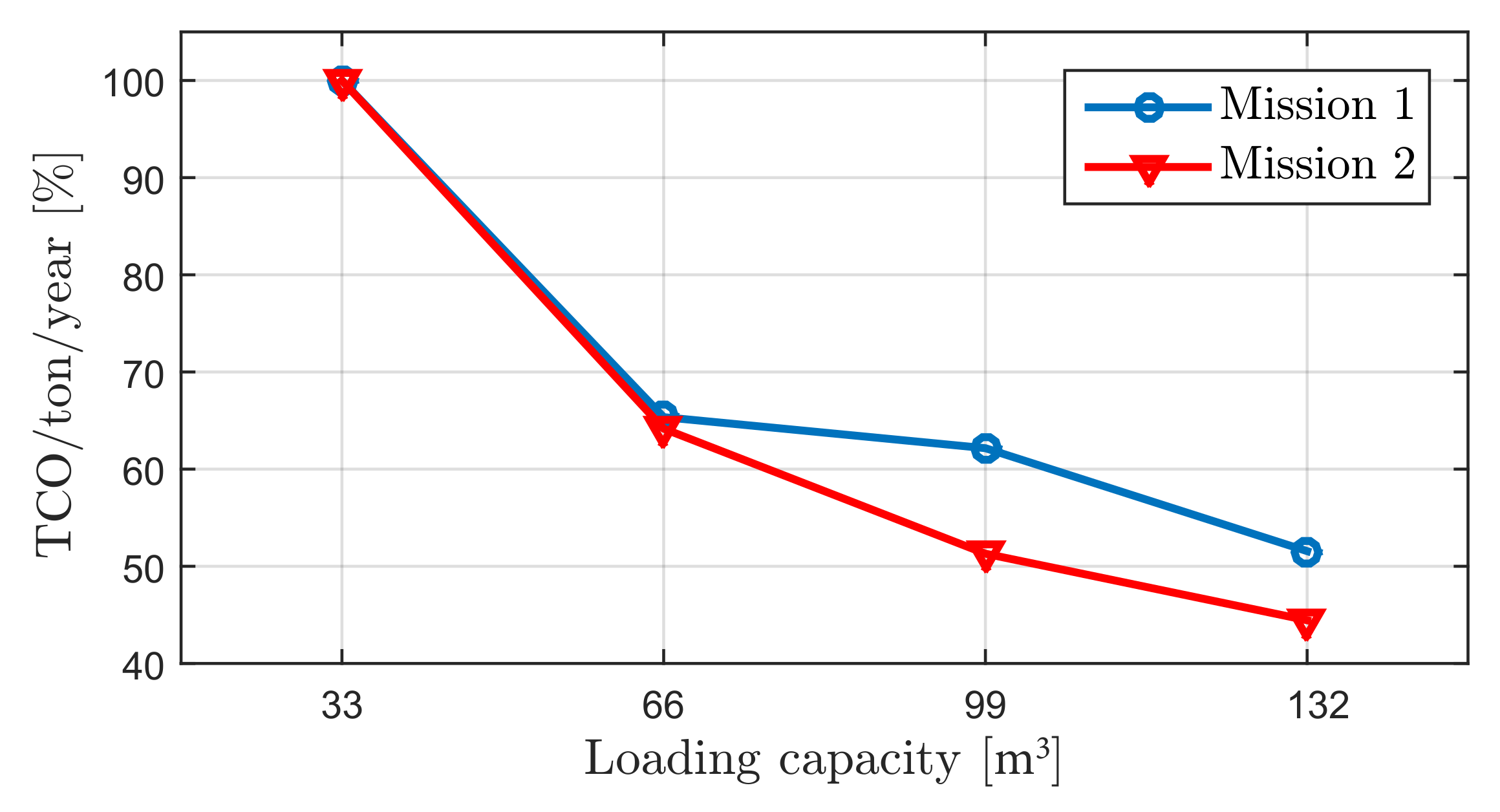
Finally, Figure 18 compares annual costs of transportation per ton of freight amongst optimally designed vehicles of different sizes. The largest vehicle demonstrated an average 53% reduction in costs compared to the smallest vehicle. Large vehicles were observed to perform even better during the second mission compared to the first, since they tend to spend less time in loading–unloading during the second mission, thereby resulting in higher vehicle utilization. Moreover, considering the impact of driver and depreciation costs, it is usually the case that trucks with higher capacity are more attractive as long as they are not idle (low temporal utilization) or traveling partially full (low capacity utilization).

5.2. Competitiveness Amongst Conventional, Fully Electric, and Plug-in Hybrid Heavy-Vehicle Combinations

Gross combination mass (GCM) is the maximum mass of a vehicle allowed on a road. As regards the case-study problem considered in this study, loading capacities are mostly constrained by volume while the mass constraint remains inactive; thus, GCM is not realized, and the weight of battery packs does not reduce the loading capacity or capacity utilization of fully electric and hybrid vehicles compared to that of conventional vehicles. Moreover, the unit of mass [ton] is considered as a unit of transported freight while calculating the annual TCO per unit freight, thereby implying that a larger transported mass contributes to lower unit-transportation cost.

Another scenario could be considered in the form of transportation of high-density freight, so that the mass constraint becomes active. In such a case, heavy hardware reduces the overall loading capacity, thereby resulting in higher transportation cost. Besides the limited range of electric vehicles and expensive batteries, reduction in loading capacity through use of heavy hardware in both electric and hybrid vehicles makes them infeasible for use in some applications [2] although a value of total vehicle mass exceeding GCM by a small amount is allowed for electric and hybrid heavy-vehicles, in accordance with the directive (EU) 2015/719. Figure 19 depicts how the type of transported freight (low- or high-density), battery cost, and number of vehicles involved in a mission influence optimum vehicle hardware when performing different missions. As a measure of the battery cost, the number of charge-discharge cycles (NOC) performed prior to the end of battery life (EOL) was used. This measure corresponds to battery quality in that a high NOC implies lesser battery replacements needed during the service life of a vehicle (refer battery-degradation model in Appendix E). Figure 19 depicts roughly under what conditions electric and hybrid vehicles become economically more feasible compared to conventional ones. Vehicle combinations employed during missions 1, 2, and 3 demonstrated GCM values of 80, 80, and 35 tons, respectively. The loading–unloading scheme was fixed as described in Table 3. The hardware and recharging power were separately optimized for the given number of vehicles, freight type, and NOC during different missions as well as conventional, electric, and hybrid vehicle types. Likewise, costs of optimum vehicles of the conventional, hybrid, and fully electric type have been separately indicated for different missions and for two cases—volume constraint active considering low-density freight; and mass constraint active considering high-density freight. Plots on the left correspond to the case when only the volume constraint is active, similar to the case-study problem described above. Correspondingly, plots on the right depict the case with active mass constraint. Following conclusions could be drawn from the figure.

□

Electric and hybrid heavy-vehicle combinations equipped with a medium-quality battery result in lower costs compared to conventional vehicles for the case wherein only the volume constraint is active corresponding to low-density transported freight, such that GCM is not realized even when large batteries are employed.

□

Conventional heavy-vehicle combinations result in lower costs being incurred in cases wherein the mass constraint is active, i.e., no more freight can be loaded because the GCM limit is reached. In such a case, use of heavy batteries reduces the maximum freight that can be loaded.

□

To meet large demands of freight flow during a given mission, more than one vehicle may be required. Thus, the cost of recharging infrastructure can be shared, and the optimum battery size changes accordingly (refer Table 4). In such cases, fully electric and hybrid heavy-vehicle combinations come across as being cheaper, albeit equipped with a medium-quality battery while the mass constraint remains active.

□

Electric vehicles benefit more compared to hybrid vehicles from enhancement in battery quality.

□

The cost per ton of freight decreases when using better batteries, more number of vehicles, and more loaded freight per vehicle.

□

For short missions involving many stops, i.e., mission three, use of conventional vehicles results in lower unit transportation costs compared to hybrid and electric vehicles for transportation of high-density freight. This is because for transportation of heavy freight, a stronger powertrain is needed, and for a mission with multiple stops, the vehicle spends less time on the road, thereby resulting low vehicle temporal utilization. Thus, the depreciation cost of expensive hybrid and electric powertrains, or purchase cost, is higher compared to that of conventional powertrains, as also reported by [20].

□

As a result of simultaneous optimization, a fleet of fully electric heavy-vehicle combinations can be designed with approximately 5–10% reduction in TCO compared to a fleet of conventional vehicles.

It must also be noted that the unit transportation cost of electric and hybrid vehicles increases if the working time per day is short owing to the high depreciation cost of hardware and low vehicle temporal utilization. In such a case, the vehicle is not used enough to return the cost of investment. Furthermore, tax incentives, future reduction in battery price, increase in diesel price, and extension of vehicle service life or planning horizon all contribute to even cheaper and more competitive electric heavy-vehicle combinations being made available in the near future. Moreover, fuel efficiency and cost are among reasons of coupling between transportation and vehicle design as well as dependence of optimum vehicle hardware to specific use-case (depending on the cost of fuel in region being studied) [5,29].

6. Discussion and Remarks

The following remarks are relevant to the limitations and clarifications of the suggested methodology.

–

The optimizer might increase the size of batteries more than the needed traveling range and power to minimize the number of battery replacements required during the service life of a vehicle.

–

Recharging-power design is only performed for daily operation of a vehicle. The charging power and number of charging plugs required while, for example, all vehicles are not in operation (i.e., during night), are not considered. However, battery degradation owing to overnight charging has been considered in this study.

–

When employing hybrid vehicles, operational costs could be reduced by implementing an optimum energy-management strategy (OEMS), which whilst considering upcoming driving horizon, optimally splits requested power between electric motors and ICE. However, for vehicle configurations identified for operation in smooth traffic, OEMS gain was observed to be less than 4% in terms of reduction in energy and battery-degradation costs [49]. More specifically, for the first mission, the gain is close to zero owing to the large battery size; during the second mission, an approximately 3% gain is observed; lastly, during the third mission, the observed gain again nearly equals zero owing mainly to availability of a near-flat road. In this study, the coupling between OEMS and vehicle-infrastructure design has not been considered. Considering OEMS and an optimum-speed profile together with vehicle-infrastructure design, the optimization exercise might result in the design of hybrid vehicles equipped with smaller batteries as a feasible solution.

–

A driver can rest during the loading–unloading process. In the case study, the waiting time at seaport is 90 min, which the driver utilizes for resting.

–

It has been observed that TCO increased up to 30% if an optimum fully-electric vehicle designed to operate in the first mission is used, instead, in the third mission, while the optimum loading capacity is kept similar to the one in the third mission, for both cases.

It should be noted that the best vehicle-infrastructure candidates identified during each mission are exclusively applicable for that mission irrespective of all other missions. This leads to a problem when two different designs are finalized for the loading–unloading scheme at a node shared between two missions. Furthermore, optimum vehicle-infrastructure candidates of a given size are determined exclusively for that size irrespective of other vehicles with different sizes employed in the same mission. The ownership cost of a mission is a nonlinear function of the total number of vehicles employed with different loading capacities. Moreover, charging infrastructure and semitrailers or straddle carriers could be shared among all vehicles involved in a mission, not only among vehicles with the same loading capacity, as was earlier assumed while building the look-up space. The latter problem, however, is not very significant, since there always exists one vehicle size that is dominant in a given mission. If multiple vehicles are needed, they would all be of the same size whilst only one or two vehicles with sizes different compared to dominant one would be employed to fulfill an uneven total demand of freight flow.

The first problem could be overcome by redesigning missions comprising shared nodes with different loading–unloading and/or charging infrastructure designs. The highest redesign priority is assigned to the mission with lower infrastructure cost whilst using information already available from other designed missions.

Another alternative of problem definition is employing a flexible working time constraint, wherein working is allowed more than the maximum daily working time, however, with a penalty on operational costs. Consequently, a parabolic-like cost curve as a function of number of trips per day was observed. If there exists no penalty cost for violating the flexible time window, there would be a steady decrease in cost whit respect to number of trips. In the latter case, annual TCO per unit of freight [ton] can be minimized to find the optimized fleet. However, in the former case, there should be another optimization process which distributes the total number of trips among vehicles, assigning the optimum number of trips to as many vehicles as possible. Figure 20 shows the dependence of the annual cost per freight unit to the number of vehicles and number of trips each vehicle performs, for two cases. First case introduces no-penalty costs; while in the second case, a 50% penalty on operational cost for working time more than eight hours has been introduced.

For an excising carrier fleet, with already known vehicle hardware, to apply the framework described in this study, the range of vehicle powertrain decision variables need to be fixed and the rest of the optimization framework can be applied with no change.

Despite the small size of the transportation network in the case-study, the problem cannot be solved by enumeration. There are approximately 83,000 vehicle types, whereas the number of vehicles and number of trips are unknowns. Assuming maximum 10 vehicles of each type and 10 trips of each vehicle on a route yields ${(10\times 10)}^{83,000}$ different possibilities for a single route. In addition, the case study included at least four missions, on average two routes per mission, six nodes each with an unknown charging power from a set of 18 choices ($6\times 18$ different possibilities) and unknown loading–unloading (four different possibilities). Therefore, the total number of possibilities is approximately $(4\times 2\times 6\times 18\times 6\times 4)\times {(10\times 10)}^{83,000}\approx {10}^{166,000}$. Clearly, such a problem cannot be solved by enumeration because of many different possibilities.

Finally, it must be noted that the presented values are only valid for the missions defined, input data provided, and vehicle models used. However, the methodology of determining the optimum fleet is generally applicable for repetitive transportation assignments and may be modified to include more vehicle- and transportation-design variables; for instance, type of gearbox, location of articulation point(s), inclusion of dynamic charging [65], more options of loading–unloading and charging strategy.

Limitations

In this study, the driving cycle of all trips is considered to be fully deterministic and no variation in traffic due to nondeterministic events has been considered. In case of a high probability of deviation from a given driving cycle (owing to heavy traffic, for example), higher constraints on vehicle performance must be applied.

The solution method described in this paper is based on a given set of missions ${\mathit{X}}_{\mathrm{m}}$ as an input. In case of dealing with a transportation network of low number of route connectivity, the number of possible missions included in ${\mathit{X}}_{\mathrm{m}}$ is low, thereby making the method presented in this paper computationally applicable. However, the method can still be useful for large transportation networks if the number of possible missions or the number of cyclic routes can be reduced by means of a bounding procedure, which allows only potential “good” routes in the ${\mathit{X}}_{\mathrm{r}}$ set. The potential “good” routes could be determined by decoupling the two problems of routing and vehicle-infrastructure design in a large transportation network. Such a decoupling has been motivated by the results reported in [40] stating that, in presence of performance constraints, routing problem is not strongly interconnected with vehicle design. Traditional approaches for solving VRPs could then be employed on a small set of representative vehicle types. For example, a homogeneous VRP reported by [66] can be solved separately for each available loading capacity using a representative vehicle hardware setup. A combination of all separate solutions along with corresponding solutions for heterogeneous VRPs on the same representative set of vehicles yields a reduced set of routes/missions.

In addition, potential “good” missions can be determined by solving network optimization problems or districting [67]. As such, output districts—a group of nodes that could be visited by a single vehicle—serve as inputs to the set of missions, wherein a mission is either defined by a single or multiple cyclic routes corresponding to multiple trips or by a district with several possible cyclic routes.

In the proposed study, the authors have tried to include most aspects important to transportation systems; however, not all aspects could be considered—speed optimization, for example. As reported by [68], allowing a heterogeneous fleet is more important than speed optimization on each arc, and using a fixed speed results in slightly higher energy-consumption compared to moving at an optimized speed. This claim is true for combustion-powered vehicles with fixed hardware running on flat roads. For a vehicle moving on a road with variable grade, having the speed as an optimization variable is useful, as reported by [69,70]. However, speed optimization is not considered in this study owing to increased complexity and computational cost. The effect of average speed on vehicle-infrastructure design is studied in ref. [11].

The approach presented in this study yields an efficient and low-cost vehicle-transportation if the vehicle use-case is known during the entire or dominant part of its lifetime. If transportation characteristics, i.e., consumers, routes, the characteristics of the roads, amounts and types of goods transported etc would change considerably over the lifetime of a vehicle, optimizing towards a very specific operation would lead to inefficiency and even in-feasibility in other transport operations. Therefore, to keep the vehicles to operate near their best performance, the deviation from the assignments that they are designed for has to be small.

7. Conclusions

The proposed study demonstrates that vehicle hardware design can be treated as an integrated optimization problem comprising transportation-mission, logistics, infrastructure, and fleet-size optimization. A case-study problem has been solved according to the proposed methodology. It has been demonstrated that freight-vehicle designs are influenced by the route, transportation mission, fleet-size and recharging power, as well as transportation boundaries, such as loading–unloading schemes, especially in case of battery-electric heavy-vehicle. Moreover, use of an integrated optimization process could lead to increased profitability of battery-electric heavy-vehicle combinations in highway and urban freight transport by about 30%, and up to 10% reduction in TCO compared to a fleet of conventional vehicles. In addition, it has been shown that long heavy-vehicle combinations in a heterogeneous fleet result in an approximate 53% reduction in TCO compared to a homogeneous fleet comprising rigid trucks. The final outcome of the optimization process is a vehicle fleet with minimum TCO and zero emissions provided that electric energy comes from renewable sources and ignoring emissions from vehicle and particularly battery manufacturing. Through use of the proposed integrated fleet design, this study demonstrates that battery-electric heavy-vehicle combinations can compete against their conventional combustion-powered counterparts, and discusses contributing factors such as vehicle utilization level, payload, battery quality, number of vehicles, battery size and charging power. This would create a true incentive for transportation companies to consider switching to electrification.

The resulting optimization problem is very large; thus, a methodology has been proposed to reduce its size by defining and solving several much smaller optimization subproblems. The first stage includes finding the best vehicle-infrastructure candidates, and in the second stage, the final fleet is found among those candidates and corresponding missions and number of trips are assigned. The proposed methodology is limited to the availability of a clear description of a relatively small transportation network and repetitive assignments, that must be obtained through clear communication between stakeholders, already in conceptual design stages of the vehicles.

References

1. Hoff, A.; Andersson, H.; Christiansen, M.; Hasle, G.; Løkketangen, A. Industrial aspects and literature survey: Fleet composition and routing. Comput. Oper. Res. 2010, 37, 2041–2061. [Google Scholar] [CrossRef] [Green Version]
2. Taefi, T.T.; Kreutzfeldt, J.; Held, T.; Konings, R.; Kotter, R.; Lilley, S.; Baster, H.; Green, N.; Laugesen, M.S.; Jacobsson, S.; et al. Comparative Analysis of European Examples of Freight Electric Vehicles Schemes—A Systematic Case Study Approach with Examples from Denmark, Germany, the Netherlands, Sweden and the UK. In Dynamics in Logistics; Springer: Cham, Switzerland, 2016; pp. 495–504. [Google Scholar]
3. Pelletier, S.; Jabali, O.; Laporte, G. 50th anniversary invited article—Goods distribution with electric vehicles: Review and research perspectives. Transp. Sci. 2016, 50, 3–22. [Google Scholar] [CrossRef]
4. Shepherd, S.; Bonsall, P.; Harrison, G. Factors affecting future demand for electric vehicles: A model based study. Transp. Policy 2012, 20, 62–74. [Google Scholar] [CrossRef]
5. Taefi, T.T.; Kreutzfeldt, J.; Held, T.; Fink, A. Strategies to increase the profitability of electric vehicles in urban freight transport. In E-Mobility in Europe; Springer: Cham, Switzerland, 2015; pp. 367–388. [Google Scholar]
6. Edlund, S.; Fryk, P.O. The Right Truck for the Job with Global Truck Application Descriptions; Technical Report, SAE Technical Paper; SAE: Warrendale, PA, USA, 2004. [Google Scholar]
7. Pettersson, P.; Berglund, S.; Ryberg, H.; Jacobson, B.; Karlsson, G.; Brusved, L.; Bjernetun, J. Comparison of dual and single clutch transmission based on Global Transport Application mission profiles. Int. J. Veh. Des. 2018, 77, 22–42. [Google Scholar] [CrossRef]
8. Iwan, S.; Małecki, K. Data flows in an integrated urban freight transport telematic system. In Proceedings of the International Conference on Transport Systems Telematics, Ustron, Poland, 10–13 October 2012; Springer: Berlin/Heidelberg, Germany, 2012; pp. 79–86. [Google Scholar]
9. Iwan, S.; Małecki, K.; Korczak, J. Impact of telematics on efficiency of urban freight transport. In Proceedings of the International Conference on Transport Systems Telematics, Ustron, Poland, 23–26 October 2013; Springer: Berlin/Heidelberg, Germany, 2013; pp. 50–57. [Google Scholar]
10. Kijewska, K.; Iwan, S.; Małecki, K. Applying multi-criteria analysis of electrically powered vehicles implementation in urban freight transport. Procedia Comput. Sci. 2019, 159, 1558–1567. [Google Scholar] [CrossRef]
11. Ghandriz, T.; Jacobson, B.; Laine, L.; Hellgren, J. Impact of automated driving systems on road freight transport and electrified propulsion of heavy vehicles. Transp. Res. Part C Emerg. Technol. 2020, 115, 102610. [Google Scholar] [CrossRef]
12. Aurell, J.; Wadman, T. Vehicle Combinations Based on the Modular Concept; Nordiska Vägteknisk Förbundet (Nordic Road Assoc): Gothenburg, Sweden, 2007; Volume 1. [Google Scholar]
13. Demir, E.; Bektaş, T.; Laporte, G. A review of recent research on green road freight transportation. Eur. J. Oper. Res. 2014, 237, 775–793. [Google Scholar] [CrossRef] [Green Version]
14. Baldacci, R.; Toth, P.; Vigo, D. Recent advances in vehicle routing exact algorithms. 4OR 2007, 5, 269–298. [Google Scholar] [CrossRef]
15. Koç, Ç.; Bektaş, T.; Jabali, O.; Laporte, G. Thirty years of heterogeneous vehicle routing. Eur. J. Oper. Res. 2016, 249, 1–21. [Google Scholar] [CrossRef] [Green Version]
16. Goeke, D.; Schneider, M. Routing a mixed fleet of electric and conventional vehicles. Eur. J. Oper. Res. 2015, 245, 81–99. [Google Scholar] [CrossRef]
17. Kopfer, H.; Vornhusen, B. Energy vehicle routing problem for differently sized and powered vehicles. J. Bus. Econ. 2019, 64, 793–821. [Google Scholar] [CrossRef]
18. Desaulniers, G.; Errico, F.; Irnich, S.; Schneider, M. Exact algorithms for electric vehicle-routing problems with time windows. Oper. Res. 2016, 64, 1388–1405. [Google Scholar] [CrossRef]
19. Sassi, O.; Cherif, W.R.; Oulamara, A. Vehicle Routing Problem with Mixed Fleet of Conventional and Heterogenous Electric Vehicles and Time Dependent Charging Costs. Available online: https://hal.archives-ouvertes.fr/hal-01083966 (accessed on 18 December 2018).
20. Davis, B.A.; Figliozzi, M.A. A methodology to evaluate the competitiveness of electric delivery trucks. Transp. Res. Part E Logist. Transp. Rev. 2013, 49, 8–23. [Google Scholar] [CrossRef]
21. Hiermann, G.; Puchinger, J.; Ropke, S.; Hartl, R.F. The electric fleet size and mix vehicle routing problem with time windows and recharging stations. Eur. J. Oper. Res. 2016, 252, 995–1018. [Google Scholar] [CrossRef] [Green Version]
22. Strehler, M.; Merting, S.; Schwan, C. Energy-efficient shortest routes for electric and hybrid vehicles. Transp. Res. Part B Methodol. 2017, 103, 111–135. [Google Scholar] [CrossRef]
23. Taefi, T.T.; Kreutzfeldt, J.; Held, T.; Fink, A. Supporting the adoption of electric vehicles in urban road freight transport–A multi-criteria analysis of policy measures in Germany. Transp. Res. Part A Policy Pract. 2016, 91, 61–79. [Google Scholar] [CrossRef]
24. Tavakkoli-Moghaddam, R.; Safaei, N.; Kah, M.; Rabbani, M. A new capacitated vehicle routing problem with split service for minimizing fleet cost by simulated annealing. J. Frankl. Inst. 2007, 344, 406–425. [Google Scholar] [CrossRef]
25. Teodorovic, D.; Krcmar-Nozic, E.; Pavkovic, G. The mixed fleet stochastic vehicle routing problem. Transp. Plan. Technol. 1995, 19, 31–43. [Google Scholar] [CrossRef]
26. Feng, W.; Figliozzi, M. An economic and technological analysis of the key factors affecting the competitiveness of electric commercial vehicles: A case study from the USA market. Transp. Res. Part Emerg. Technol. 2013, 26, 135–145. [Google Scholar] [CrossRef]
27. Wu, G.; Inderbitzin, A.; Bening, C. Total cost of ownership of electric vehicles compared to conventional vehicles: A probabilistic analysis and projection across market segments. Energy Policy 2015, 80, 196–214. [Google Scholar] [CrossRef]
28. Taefi, T.T.; Stütz, S.; Fink, A. Assessing the cost-optimal mileage of medium-duty electric vehicles with a numeric simulation approach. Transp. Res. Part D Transp. Environ. 2017, 56, 271–285. [Google Scholar] [CrossRef]
29. Lee, D.Y.; Thomas, V.M.; Brown, M.A. Electric urban delivery trucks: Energy use, greenhouse gas emissions, and cost-effectiveness. Environ. Sci. Technol. 2013, 47, 8022–8030. [Google Scholar] [CrossRef]
30. Botsford, C.; Szczepanek, A. Fast charging vs. slow charging: Pros and cons for the new age of electric vehicles. In Proceedings of the International Battery Hybrid Fuel Cell Electric Vehicle Symposium, Stavanger, Norway, 13–16 May 2009. [Google Scholar]
31. Nesterova, N.; Quak, H.; Balm, S.; Roche-Ceraso, I.; Tretvik, T. State of the Art of the Electric Freight Vehicles Implementation in City Logistics; FREVUE Project Deliverable D; European Commission: Brussels, Belgium, 2013; Volume 1. [Google Scholar]
32. Hovgard, M.; Jonsson, O.; Murgovski, N.; Sanfridson, M.; Fredriksson, J. Cooperative energy management of electrified vehicles on hilly roads. Control. Eng. Pract. 2018, 73, 66–78. [Google Scholar] [CrossRef]
33. Lebeau, P.; Macharis, C.; Van Mierlo, J.; Lebeau, K. Electrifying light commercial vehicles for city logistics? A total cost of ownership analysis. Eur. J. Transp. Infrastruct. Res. 2015, 15. [Google Scholar] [CrossRef]
34. Hagman, J.; Ritzén, S.; Stier, J.J.; Susilo, Y. Total cost of ownership and its potential implications for battery electric vehicle diffusion. Res. Transp. Bus. Manag. 2016, 18, 11–17. [Google Scholar] [CrossRef] [Green Version]
35. Wadud, Z. Fully automated vehicles: A cost of ownership analysis to inform early adoption. Transp. Res. Part A Policy Pract. 2017, 101, 163–176. [Google Scholar] [CrossRef]
36. Palmer, K.; Tate, J.E.; Wadud, Z.; Nellthorp, J. Total cost of ownership and market share for hybrid and electric vehicles in the UK, US and Japan. Appl. Energy 2018, 209, 108–119. [Google Scholar] [CrossRef]
37. Lebeau, P.; Macharis, C.; Van Mierlo, J. How to Improve the Total Cost of Ownership of Electric Vehicles: An Analysis of the Light Commercial Vehicle Segment. World Electr. Veh. J. 2019, 10, 90. [Google Scholar] [CrossRef] [Green Version]
38. Küng, L.; Bütler, T.; Georges, G.; Boulouchos, K. Decarbonizing passenger cars using different powertrain technologies: Optimal fleet composition under evolving electricity supply. Transp. Res. Part C Emerg. Technol. 2018, 95, 785–801. [Google Scholar] [CrossRef]
39. Kontou, E.; Yin, Y.; Lin, Z.; He, F. Socially optimal replacement of conventional with electric vehicles for the US household fleet. Int. J. Sustain. Transp. 2017, 11, 749–763. [Google Scholar] [CrossRef]
40. Ghandriz, T.; Hellgren, J.; Islam, M.; Laine, L.; Jacobson, B. Optimization based design of heterogeneous truck fleet and electric propulsion. In Proceedings of the 2016 IEEE 19th International Conference on Intelligent Transportation Systems (ITSC), Rio de Janeiro, Brazil, 1–4 November 2016; pp. 328–335. [Google Scholar]
41. Li, F.; Golden, B.; Wasil, E. A record-to-record travel algorithm for solving the heterogeneous fleet vehicle routing problem. Comput. Oper. Res. 2007, 34, 2734–2742. [Google Scholar] [CrossRef]
42. Choi, E.; Tcha, D.W. A column generation approach to the heterogeneous fleet vehicle routing problem. Comput. Oper. Res. 2007, 34, 2080–2095. [Google Scholar] [CrossRef]
43. Baldacci, R.; Mingozzi, A. A unified exact method for solving different classes of vehicle routing problems. Math. Program. 2009, 120, 347. [Google Scholar] [CrossRef]
44. Kopfer, H.W.; Schönberger, J.; Kopfer, H. Reducing greenhouse gas emissions of a heterogeneous vehicle fleet. Flex. Serv. Manuf. J. 2014, 26, 221–248. [Google Scholar] [CrossRef]
45. Arslan, O.; Karaşan, O.E. A Benders decomposition approach for the charging station location problem with plug-in hybrid electric vehicles. Trans. Res. Part B Methodol. 2016, 93, 670–695. [Google Scholar] [CrossRef] [Green Version]
46. Benders, J.F. Partitioning procedures for solving mixed-variables programming problems. Numer. Math. 1962, 4, 238–252. [Google Scholar] [CrossRef]
47. Barman, S.E.; Lindroth, P.; Strömberg, A.B. Modeling and solving vehicle routing problems with many available vehicle types. In Optimization, Control, and Applications in the Information Age; Springer: Cham, Switzerland, 2015; pp. 113–138. [Google Scholar]
48. Ghandriz, T.; Jacobson, B. A Vehicle Longitudinal Dynamical Model for Propulsion Component Tailoring; Technical Report; Chalmers University of Technology: Gothenburg, Sweden, 2020. [Google Scholar]
49. Ghandriz, T.; Laine, L.; Hellgren, J.; Jacobson, B. Sensitivity analysis of optimal energy management in plug-in hybrid heavy vehicles. In Proceedings of the 2017 2nd IEEE International Conference on Intelligent Transportation Engineering (ICITE), Singapore, 1–3 September 2017; pp. 320–327. [Google Scholar]
50. Montoya, A.; Guéret, C.; Mendoza, J.E.; Villegas, J.G. The electric vehicle routing problem with nonlinear charging function. Trans. Res. Part B Methodol. 2017, 103, 87–110. [Google Scholar] [CrossRef] [Green Version]
51. Wang, J.; Liu, P.; Hicks-Garner, J.; Sherman, E.; Soukiazian, S.; Verbrugge, M.; Tataria, H.; Musser, J.; Finamore, P. Cycle-life model for graphite-LiFePO4 cells. J. Power Sources 2011, 196, 3942–3948. [Google Scholar] [CrossRef]
52. Hu, X.; Johannesson, L.; Murgovski, N.; Egardt, B. Longevity-conscious dimensioning and power management of the hybrid energy storage system in a fuel cell hybrid electric bus. Appl. Energy 2015, 137, 913–924. [Google Scholar] [CrossRef]
53. Pelletier, S.; Jabali, O.; Laporte, G.; Veneroni, M. Battery degradation and behaviour for electric vehicles: Review and numerical analyses of several models. Trans. Res. Part B Methodol. 2017, 103, 158–187. [Google Scholar] [CrossRef]
54. Pettersson, P. On Numerical Descriptions of Road Transport Missions; Department of Mechanics and Maritime Sciences, Vehicle Engineering and Autonomous Systems, Chalmers University of Technology: Gothenburg, Sweden, 2017. [Google Scholar]
55. Edgar, J.; Prem, H.; Calvert, F. Applying performance standards to the Australian heavy vehicle fleet. In Proceedings of the 7th International Symposium on Heavy Vehicle Weights & Dimensions, Delft, The Netherlands, 16–20 June 2002; pp. 73–96. [Google Scholar]
56. Sadeghi Kati, M. Definitions of Performance Based Characteristics for Long Heavy Vehicle Combinations; Technical Report; Chalmers University of Technology: Gothenburg, Sweden, 2013. [Google Scholar]
57. Sadeghi Kati, M.; Fredriksson, J.; Laine, L.; Jacobson, B. Evaluation of Dynamical Behaviour of Long Heavy Vehicles Using Performance Based Characterstics. In Proceedings of the FISITA 2014 World Automotive Congress, Maastricht, The Netherlands, 2–6 June 2014. [Google Scholar]
58. Kharrazi, S.; Karlsson, R.; Sandin, J.; Aurell, J. Performance Based Standards for High Capacity Transports in Sweden; FIFFI Project 2013-03881, Report 1: Review of Existing Regulations and Literature; VTI: Linköping, Sweden, 2015. [Google Scholar]
59. Baldacci, R.; Bodin, L.; Mingozzi, A. The multiple disposal facilities and multiple inventory locations rollon–rolloff vehicle routing problem. Comput. Oper. Res. 2006, 33, 2667–2702. [Google Scholar] [CrossRef]
60. Wahde, M. Biologically Inspired Optimization Methods: An Introduction; WIT Press: Southampton, UK, 2008. [Google Scholar]
61. Rios, L.M.; Sahinidis, N.V. Derivative-free optimization: A review of algorithms and comparison of software implementations. J. Glob. Optim. 2013, 56, 1247–1293. [Google Scholar] [CrossRef] [Green Version]
62. Ghandriz, T.; Jacobson, B.; Laine, L.; Hellgren, J. Optimization data on total cost of ownership for conventional and battery electric heavy vehicles driven by human and by Automated Driving Systems. Data Brief 2020, 30, 105566. [Google Scholar] [CrossRef]
63. Roso, V. Evaluation of the dry port concept from an environmental perspective: A note. Transp. Res. Part D Transp. Environ. 2007, 12, 523–527. [Google Scholar] [CrossRef]
64. Roso, V.; Woxenius, J.; Lumsden, K. The dry port concept: Connecting container seaports with the hinterland. J. Transp. Geogr. 2009, 17, 338–345. [Google Scholar] [CrossRef]
65. Alaküla, M.; Márquez-Fernández, F.J. Dynamic charging solutions in Sweden: An overview. In Proceedings of the 2017 IEEE Transportation Electrification Conference and Expo, Asia-Pacific (ITEC Asia-Pacific), Harbin, China, 7–10 August 2017; pp. 1–6. [Google Scholar]
66. Jabali, O.; Gendreau, M.; Laporte, G. A continuous approximation model for the fleet composition problem. Trans. Res. Part B Methodol. 2012, 46, 1591–1606. [Google Scholar] [CrossRef]
67. Konur, D.; Geunes, J. Integrated districting, fleet composition, and inventory planning for a multi-retailer distribution system. Ann. Oper. Res. 2016, 273, 527–559. [Google Scholar] [CrossRef]
68. Koç, Ç.; Bektaş, T.; Jabali, O.; Laporte, G. The fleet size and mix pollution-routing problem. Trans. Res. Part B Methodol. 2014, 70, 239–254. [Google Scholar] [CrossRef]
69. Ghandriz, T.; Jacobson, B.; Murgovski, N.; Nilsson, P.; Laine, L. Real-Time Predictive Energy Management of Hybrid Electric Heavy Vehicles by Sequential Programming. IEEE Trans. Veh. Technol. 2021, in press. [Google Scholar] [CrossRef]
70. Johannesson, L.; Murgovski, N.; Jonasson, E.; Hellgren, J.; Egardt, B. Predictive energy management of hybrid long-haul trucks. Control. Eng. Pract. 2015, 41, 83–97. [Google Scholar] [CrossRef]
Figure 1. Schematic of transportation network and vehicle fleet. Mission comprising nodes 0, 2, and 3 is depicted with different routes connecting the nodes marked in bold red color.
Energies 14 03221 g001
Figure 2. Example of X V —set of n v vehicle types. X V denotes the set of vehicle types and X V , i denotes ith vehicle type.
Energies 14 03221 g002
Figure 3. Example of design space S V together with vehicle and infrastructure design sets. n s denotes total number of design sets. S V , k denotes kth design set (or the range of kth design variable).
Energies 14 03221 g003
Figure 4. On-board lift.
Energies 14 03221 g004
Figure 5. Example of straddle carrier.
Energies 14 03221 g005
Figure 6. Schematic of algorithm for determining optimum fleet in two stages—(A,B). Vehicle-infrastructure optimization was repeated for each combination of mission, loading capacity and quantity of vehicle in the look-up space.
Energies 14 03221 g006
Figure 7. Look-up space S b .
Energies 14 03221 g007
Figure 8. Search space of optimization problem defined by (18)–(27). Vertical bars denote ranges of design variables.
Energies 14 03221 g008
Figure 9. Road connections of the transportation network. r k l denotes different road sections and C i denotes the ith customer. Different road colors represent different transport missions.
Energies 14 03221 g009
Figure 10. A design set of vehicles with different loading capacities. A small (33-m 3 ) container has a loading capacity of 33 m 3 or 7 tons of the intended freight. Gross combination masses are: 25, 35, 60, 80 tons from the smallest vehicle to the largest one, respectively. Semitrailers may carry two small 33-m 3 containers.
Energies 14 03221 g010
Figure 11. Optimum fleet for maximum daily working time of 10 h and daily flow of 226 m 3 ; fleet TCO equaled 287,000 €/year. LC denotes loading capacity.
Energies 14 03221 g011
Figure 12. Optimum fleet for different maximum daily working times and freight flow. Lines between nodes illustrate routes among nodes corresponding to different missions.
Energies 14 03221 g012
Figure 13. Annual cost per unit freight incurred when using optimum conventional, fully electric, and hybrid vehicles during first mission. Vehicles and corresponding missions, in which they are utilized, are marked with the same color.
Energies 14 03221 g013
Figure 14. Sensitivity of annual costs per unit freight [ton] to optimum conventional, fully electric, and hybrid vehicles separated for different cost indicators on the first mission.
Energies 14 03221 g014
Figure 15. Sensitivity of annual costs incurred per unit freight with regard to different vehicles and transportation-design parameters for different cost indicators on first mission, X r 1 .
Energies 14 03221 g015
Figure 16. Sensitivity of annual cost incurred per unit freight with regard to different loading–unloading schemes, i.e., On-Board Lift (OBL), Straddle Carrier (SC), Additional SemiTrailer (AST) On-Board vehicle Waiting (OBW) on the first mission.
Energies 14 03221 g016
Figure 17. TCO versus battery size and charging power.
Energies 14 03221 g017
Figure 18. Comparison of annual TCO savings per ton for different vehicle sizes, in case of exclusively using one vehicle size in the fleet making maximum number of trips per day within 16 h. Vehicles with 132-m 3 . loading capacity demonstrate an average 53% reduction in TCO compared to vehicles with a 33-m 3 loading capacity.
Energies 14 03221 g018
Figure 19. Competitiveness between conventional, fully electric, and hybrid vehicles in terms of the unit transportation cost of different optimally designed vehicles. Each small circle corresponds to an optimized vehicle with different hardware. For all plots, maximum working time per day is 16 h.
Energies 14 03221 g019
Figure 20. Annual transportation cost per ton as a function of number of daily trips per vehicle and number of vehicles. A penalty cost of 50% on operational cost was considered for number of trips more than four, (left); No-penalty, (right). Projection of surface lines can be seen in left and right planes.
Energies 14 03221 g020