1. Introduction
The non-destructive testing (NDT) of conveyor belts gives vast possibilities related to the optimization of conveyor belt maintenance costs, such as choosing the right moment for repair, replacement or recondition of the belt based on, among other factors, detected damage [
1] or the rate of change of belt thickness [
2]. Belt operating time depends on several factors that are presented in the literature [
2]. Among other things, it is affected by the hardness, size and shape of transported materials, the specificity of transport point and the length and age of belt cord. Some of these factors damage the belt covers or belt core.
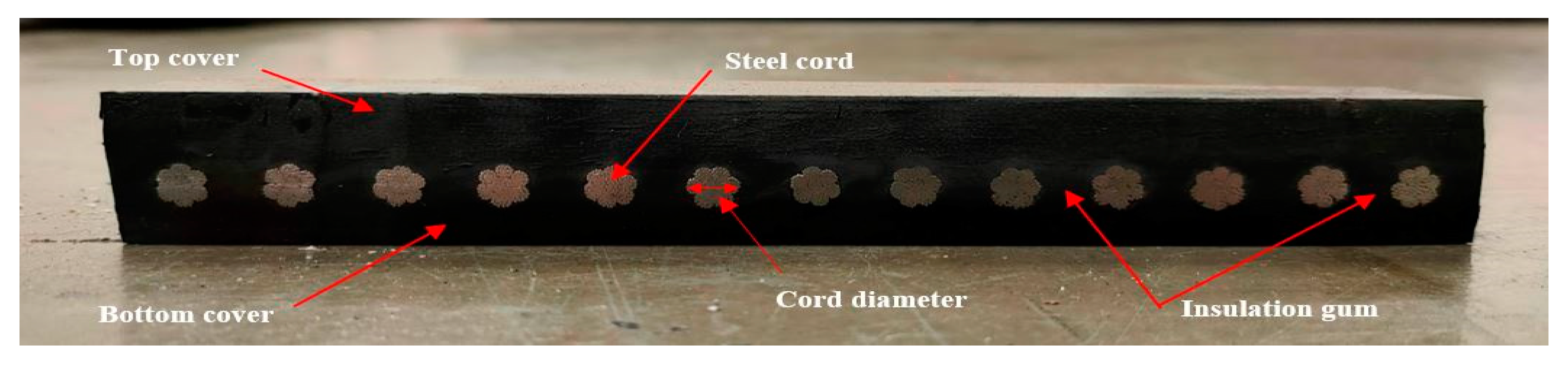
Figure 1 shows the cross-section of the example conveyor belt with steel cords.
NDT research use offers, inter alia, analysis of the magnetic field changes generated by damaged or missing cords. Research using this method has been carried out since 1970 [
3]. Since then, several researchers around the world have developed various systems to detect damage to steel cords in the belt core [
4,
5,
6]. One of the systems in use for studies is a Diagbelt magnetic system, which enables researchers to obtain two-dimensional images suitable for further analysis [
7,
8,
9]. The device detects magnetic field changes arising during the movement of cord failures beneath the measuring probe (installed across the width of the belt) which generate a discredited signal (−1, 0 or 1) corresponding to measured values of the magnetic field. The positive value of the signal measured by the device is represented in the figures presented in this paper in blue, and the signal of the negative magnetic field is represented in yellow.
For the performed comparative analysis, a reference conveyor belt containing several artificial cord failures was used. The measurements were carried out by modifying system parameters: belt speed, the distance between the measuring probe and the cord and measurement sensitivity. These parameters were selected based on previous studies [
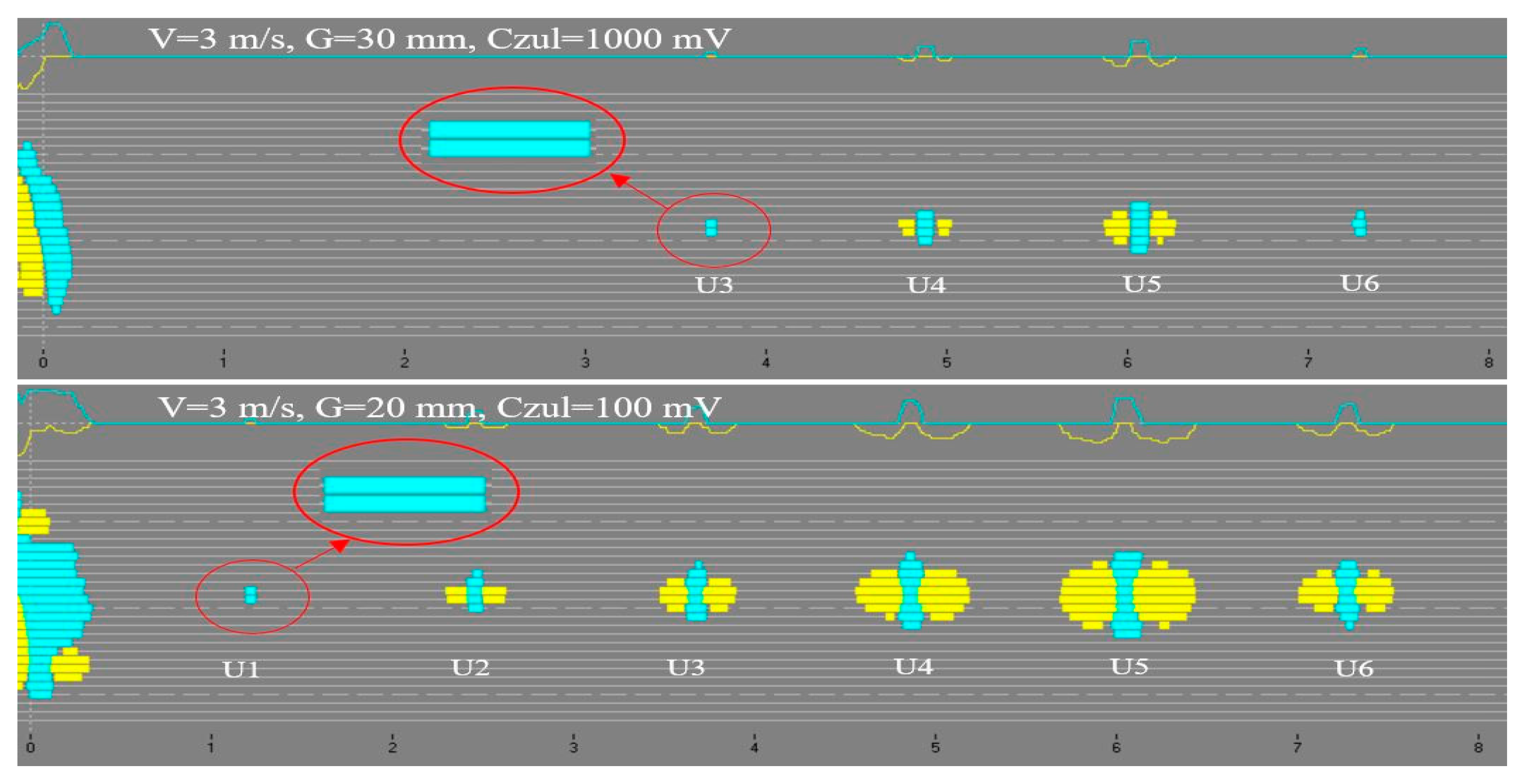
10], which have confirmed their impact on received signals. The measurements were performed for many combinations of these parameters over ten measuring cycles, of which three were selected and used for the analysis. Preliminary visual evaluation of the data indicates the relationship between failure detection signal and the above parameters. Some of the damage with the appropriate settings of parameter values generated similar signals.
Figure 2 gives an example of this situation (damage 3 and damage 1).
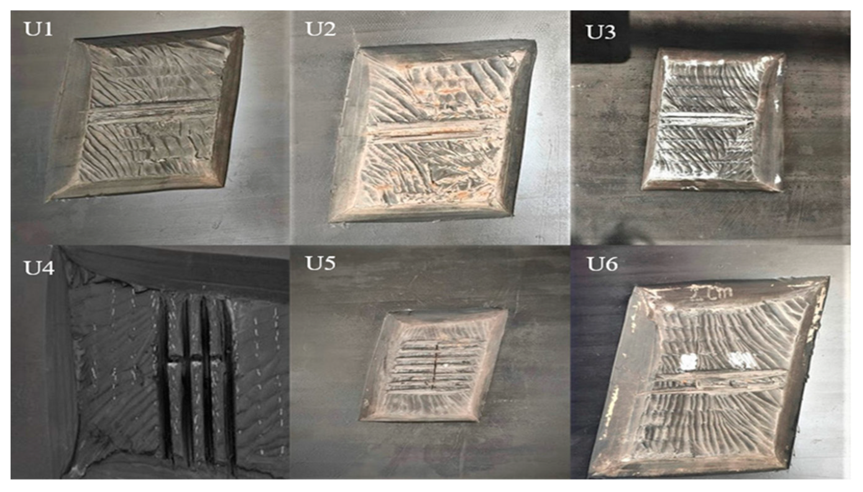
The tested failures were divided into six categories: partial cord damage (20% (U1) and 50% (U2)) in one cord, complete cut of one steel cord (U3), cut of three (U4) and six (U5) cords and resection of one cord to the length of 20 mm (U6) (
Figure 3).
2. Preparation of Data for Analysis
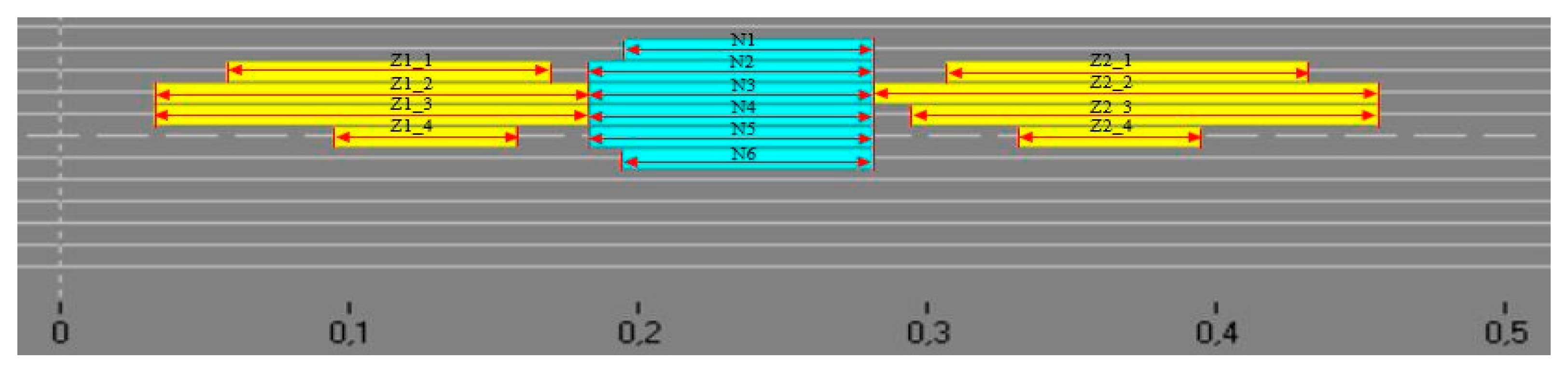
Each one of the cord failures described above generated a magnetic signal, and data were consolidated into 12 values, four for each of the sub-areas: magnetic signal surface areas, number of channels on which signal be detected, width and length of the signals. The method of calculating the size of signal for exemplary damage is shown in
Figure 4 and described by Equations (1)–(3).
where:
length of the signal detected on the
-th channel for the signal before damage,
length of the signal detected on the
-th channel for the signal of damage and
length of the signal detected on the
-th channel for the signal behind damage.
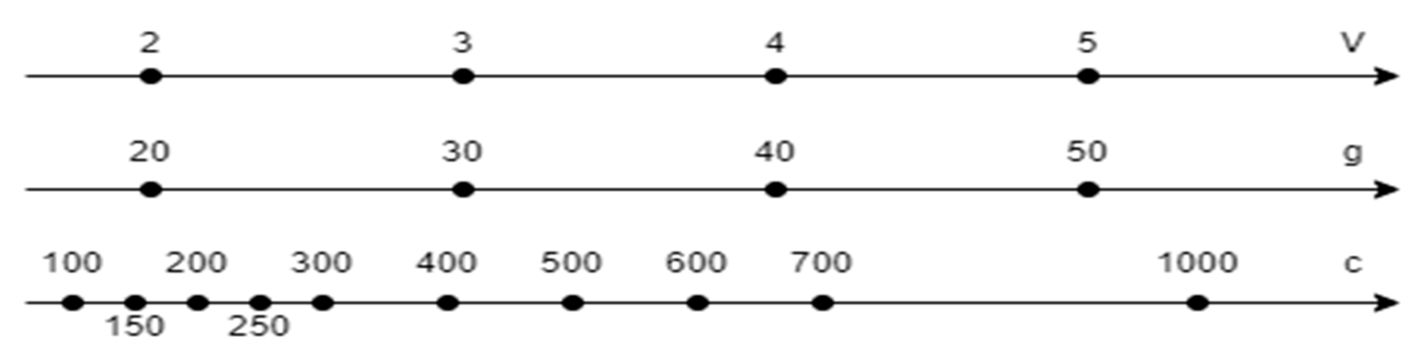
During the measurements, the belt speed (V) was increased from 2 up to 5 m/s (in increases of 1 m/s), the distance between the measuring probe and the cord (g) was changed within the range of 20–50 mm (in increases of 10 mm) and the following sensitivity levels (c) were applied: 100 mV, 150 mV, 200 mV, 250 mV, 300 mV, 400 mV, 500 mV, 600 mV, 700 mV and 1000 mV. The selection of these parameters was predicated on technical capabilities (speed of the test conveyor) and also the observation of system behaviour and its settings in numerous previous studies [
10]. The above parameter values are shown on the axis in
Figure 5.
The number of tested triple variants for given settings of the measuring system amounted to 160.
where:
—quantity of triples parameters variants,
—number of settings of sensitivity parameter,
—number of settings of belt speed and
—number of settings of distance between the measuring probe and the cord.
For each of the three measuring cycles for six defined types of damage, 2880 records describing the damage should be obtained.
where:
—theoretical number of records,
—number of measuring cycles taken into account and
—number of types of damage.
The actual amount of data was lower (2367), because magnetic field changes were not detected for less core damage in certain measurement settings.
One paper [
11] defines the most appropriate measuring system parameters, which are presented in
Table 1. For these ranges’ apparatus settings (three parameters), the number of output data sets decreased to the value of:
In reality, however, the number of records was 693 (some minor defects were not detected in specific measurement settings).
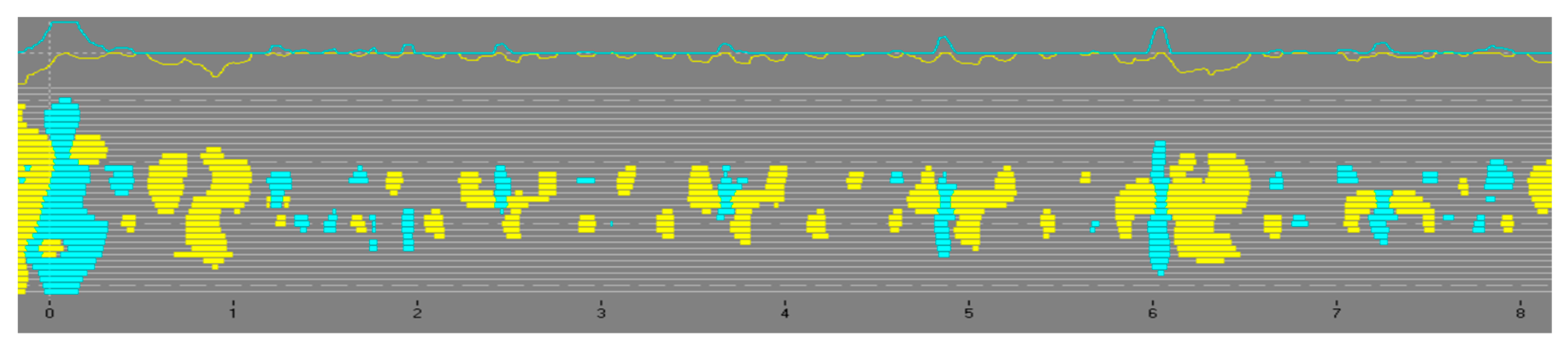
The actual sensitivities of the measuring device are inversely proportional to the parameter value called “sensitivity”. When the value of this parameter is very low (e.g., 50–100 mV), the measuring system is extremely sensitive to the slightest field changes; however, the signal produced by the device is difficult to interpret. Images of the failures fuse and also appear to measure noise (
Figure 6). Furthermore, when the value of this parameter is too large (i.e., when the system was set to be insensitive), minor damage may not have been registered, since it generates slight field changes which are outside the scope of sensitivity of the equipment.
3. Statistical Analysis
The statistical analysis was performed only for the data obtained from the optimal sets of parameters (
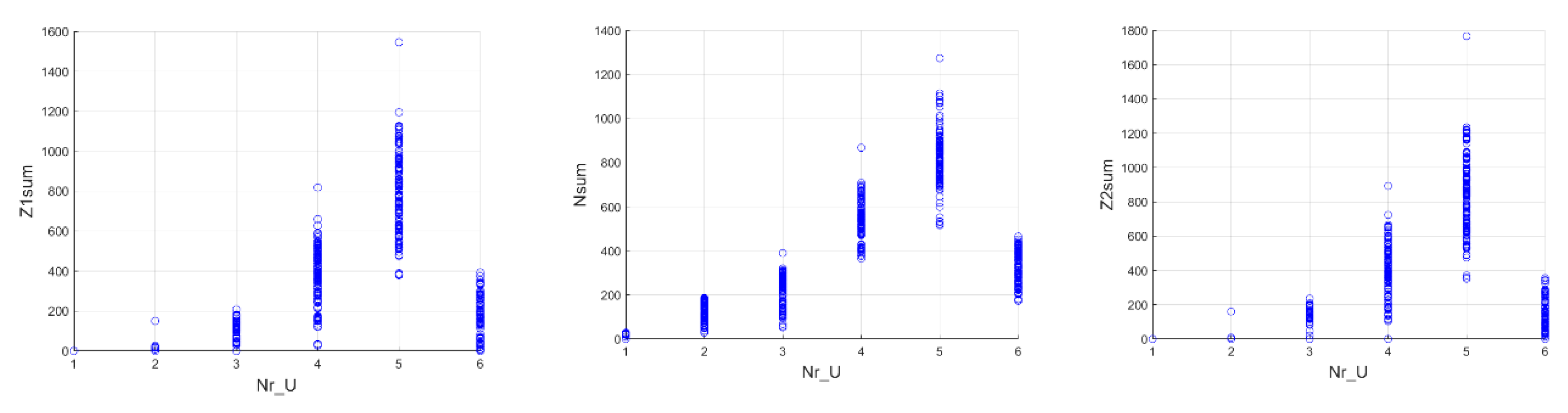
Table 2). The statistical analysis started with the verification of the obtained data to remove gross errors that may have appeared in the database, resulting, for example, from human oversight (e.g., entering incorrect data). In the next step, the correlation between the parameters taken into account in the analysis was examined. There are 13 such analysed values. They include damage number (Nr_U), number of cut cords (LL), area of damage (Pole_R), three parameters connected with the measurement system (belt speed—V, measuring probe distance—G, sensitivity—Czul), the measurement cycle taken into account (Cycle) and the failure description, including two values for each of the three damage sub-areas (yellow field before damage—Z1, blue field—N and yellow field behind the damage Z2). The measured damage parameters are the sum of the lengths of the signals recorded in the measurement channels (Z1sum, Nsum, Z2sum) and the number of channels recording the signal related to a given sub-area (Z1_LK, N_LK, Z2_LK).
Figure 7 presents charts showing the values of six measured parameters for damage depending on the class to which the damage belongs. A visual evaluation of the data helps to decide whether a given parameter affects the class differentiation or is irrelevant and can be removed.
The first part of the statistical analysis determined confidence intervals for the mean for each of the analysed measurements [
12]. Confidence intervals for the mean are given as a formula:
where:
—sample mean,
half the width of the confidence interval,
standard deviation and
number of samples.
The input base is divided into two parts: a training set and a test set. Every third value went to the test set, while the remaining samples were left in the training set. The size of the training set was 462 samples, and the size of the test set was 231.
Table 2 summarizes the calculated values that facilitate the determination of the confidence interval for each of the analysed data sets.
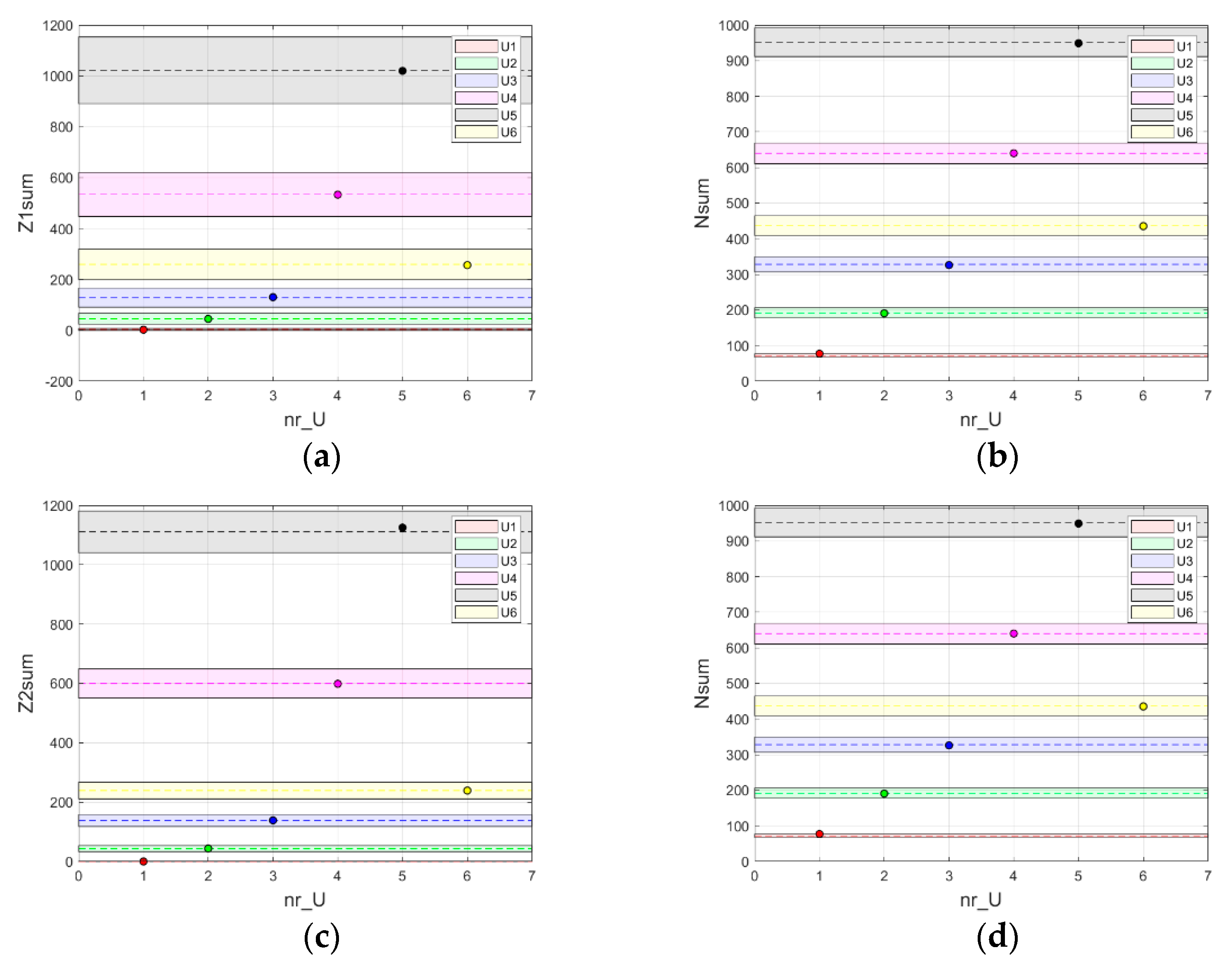
For the data from the test, the set was determined and the mean value of each of the test sets was prepared in this way. These values were placed on the graph, which also marks the widths of the determined confidence intervals (
Figure 8).
Table 3 summarizes the results obtained from a given test group. In the table, the values that fall outside the designated confidence interval are marked in red.
Therefore, it can be noticed that the problem with recognition appears only in the case of data concerning the first type of damage. The number of channels in the test sample was mean 1.00, and in the training sample was 0.88 ± 0.07.
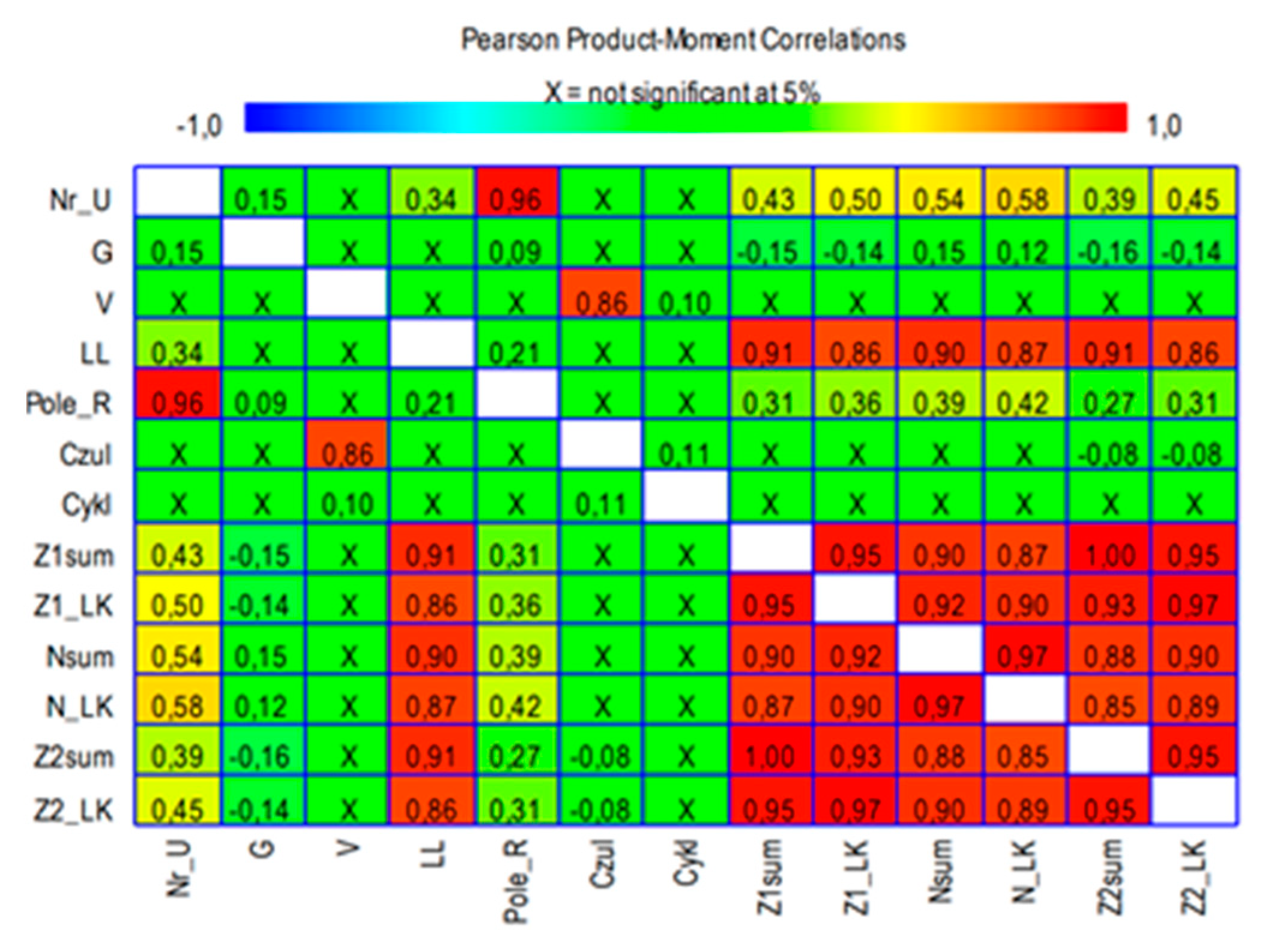
To check the influence of the analysed values on each other (their linear association), a statistical analysis was performed which determined the Pearson’s product–moment linear correlation coefficients between the setting parameters of the measurement device and the sizes of output signals for each of the analysed failures. Pearson’s correlation coefficient is a measure of linear correlation between two sets of data (the covariance of the two variables divided by the product of their standard deviations).
Figure 9 displays the estimated correlations in the form of a matrix with coloured cells. Small changes to controlled parameters and lack of outliers in results allowed us to assume the linearity of changes in results. It was applied as an initial test of linear associations for further investigations to find the physical influence of settings changes on results, to select the best settings for given working conditions of conveyor belts and to select appropriate output parameters and methods for steel cord belt failures classification.
The data in the table above (
Figure 9) are displayed using both colours and numerical values. Data marked with “X” are statistically insignificant. Coefficients define a linear relationship between two different variables. The greater the value of the correlation parameter, the greater the degree of interconnection between the pairs of variables. It is worth noting that the presented table shows that the selected parameters of the measuring system did not significantly affect the type of damage. No correlation was found between the belt speed and the measurement results (statistically insignificant correlation), there is a low correlation between the measuring head distance and the measurement results (negative or positive, depending on the area, within the range −0.16–0.15 and no significant correlation or weak negative correlation (−0.08) of the measurement results to the sensitivity of the device.
It is also worth noting that all measurement results are strongly positively correlated with each other, and the correlation between the values describing the yellow fields (Z1sum and Z2sum and Z1_LK and Z2_LK) is 1.00 and 0.97, which maintains the hypothesis about their symmetry [
1].
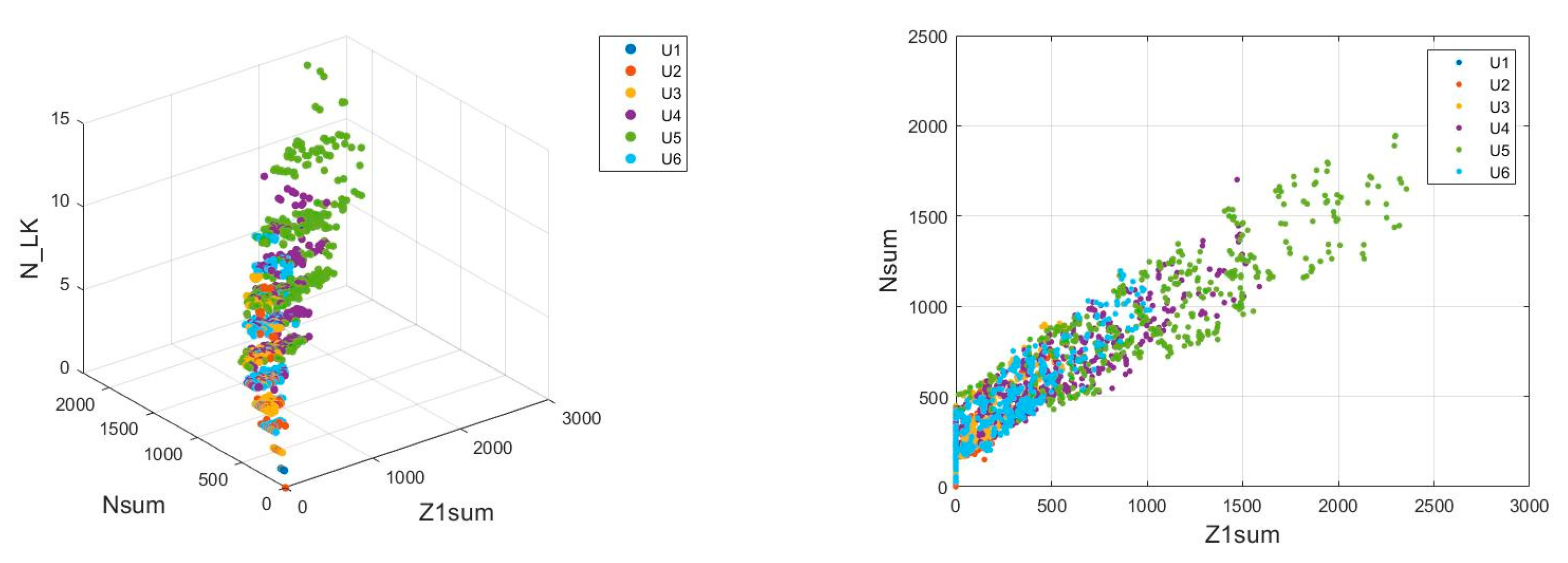
Analogical statistical analysis for the full data set was described in detail in [
13], but the results obtained there turned out to be less satisfactory than the results obtained for specific parameters of the measurement system. The distribution of the data from the complete set is shown in
Figure 10 (these graphs show the values of Z1sum, Nsum and N_LK). These results largely overlap, and it is impossible to clearly define the boundaries of clusters [
14,
15].
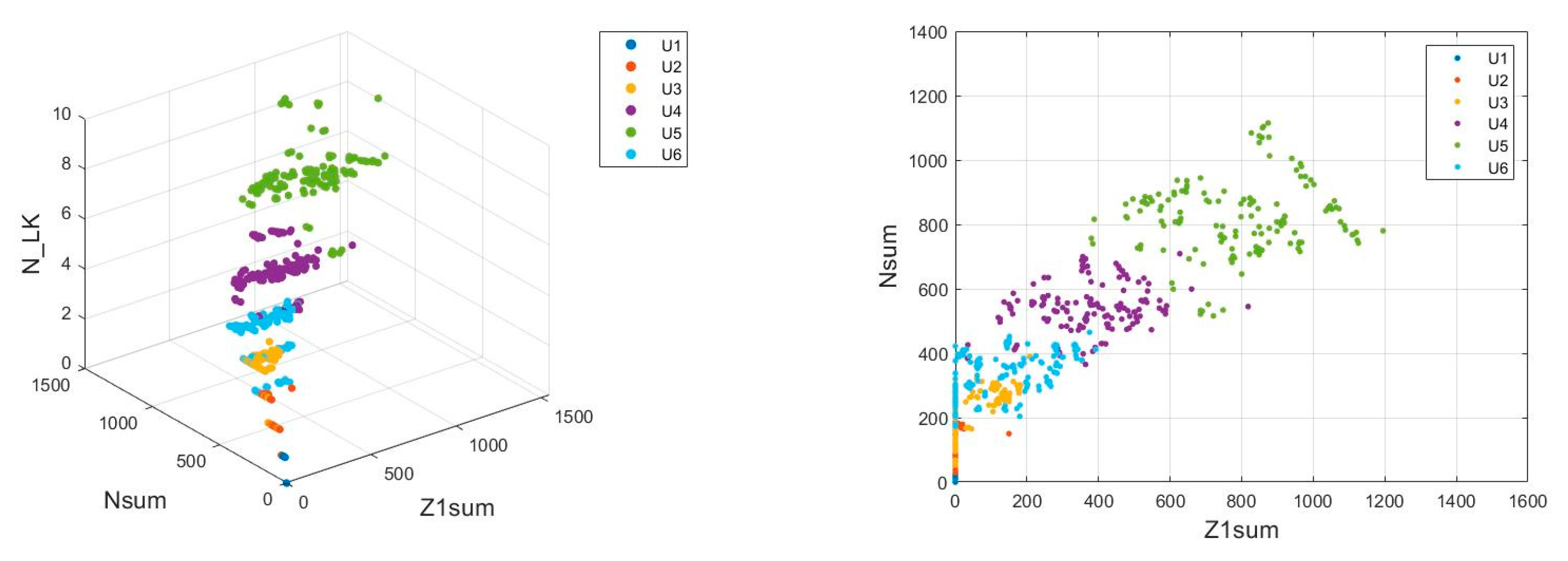
Similar graphs (
Figure 11) were also plotted for the set of parameters of the measurement system tested in this analysis. It can be noticed that, in this case, it is possible to limit the obtained data with a certain curve marking the boundary of a given cluster, although there are still areas where the belonging of the measurement result to a given cluster is ambiguous.
Optical analysis of the obtained charts shows that the measurement data are highly probable to correctly classify the type of damage, but there are areas where the classification may fail because clusters overlap [
15]. Due to this fact, another analysis was carried out using artificial neural networks.
4. Analysis with the Use of Neural Networks
The analysis of the selection of the structure and parameters of the neural network as well as the idea of its operation has been widely described in the literature. The studies [
16,
17,
18] describe in detail the rationale behind the selection of specific parameters used in this research. The MATLAB software with the Deep Learning Toolbox installed was used for the learning process of neural networks. The way of using this toolbox is described in studies [
19,
20]. This toolbox enables the creation of a multilayer neural network with a given number of neurons in each of the hidden layers, and the ability to train the neural network on a given training data set (which is automatically divided into a training and validation set). Each layer of the artificial neural network is made up of individual computing units called neurons. Neurons, stimulated by the signal fed to their input, work out the output signal using the assigned weight (
) and the added bias (
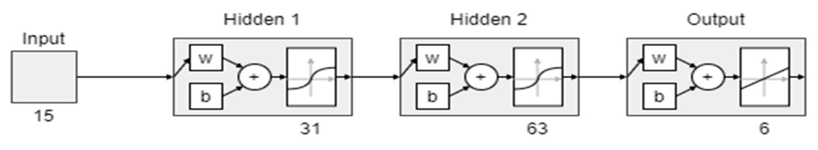
). The process of training a neural network under supervision consists of repeatedly assessing it in the process of training samples from the test set, and then updating the weight based on the error between the network response and the expected response. To use artificial neural networks to classify the conveyor belt damage, it was necessary to generate appropriate sets of training and test sets, train the network on the training set, and then test it on the test set. Since neural networks can divide the classification of space non-linearly, over the course of this research two variants of the selection and division of the input data were distinguished. In each case, the vector of input data consisted of 15 elements (and this is the number of neurons in the input layer of the neural network): 3 measurement parameters and 4 values describing each of the three sub-areas. There are 6 neurons in the output layer—one each responsible for belonging to a given class of damage. Two hidden layers consisting of 31 and 63 neurons were placed between the input and output layers. The size of these layers was determined by the Kolmogorov theorem, according to which the number of neurons in the hidden layer should be equal to the number of neurons in the previous layer multiplied by two and increased by one [
21]. The diagram of the neural network used in this study is shown in
Figure 12.
Two variants were used for the process of learning neural networks:
Each of the network learning processes in a given variant was performed three times, and the results are presented in
Table 4. The effectiveness of the diagnosis was divided depending on the type of damage that the neural network was supposed to recognize. In addition, the effectiveness of the diagnosis was also determined for the entire test set.
5. Conclusions
Many scans performed over the years using the Diagbelt system have shown that the magnetic measuring system is well suited to obtaining detailed information about the technical condition of the belt core. The idea of the system is based on the measurement of magnetic field changes at sites of core damage. The data obtained are presented on two-dimensional pictures that can be easily analysed using proposed known methodologies. The results presented in this study confirm this observation, showing the high efficiency of identification of the type of damage using the signals generated by Diagbelt.
One such method is verification based on the average of the samples. For this purpose, from the set of training data the mean value and 95% confidence interval were calculated for each damage. Then, for the test set containing the specific damage data obtained at different set values (not taken for training), the mean value was determined, which allowed for its comparison with the previously determined confidence intervals. In nearly every instance, testing set data have been included in the relevant confidence interval. The number of samples in training and testing data for selected parameter sets was 8 and 4, respectively, which could be a too-small value. It is, however, worth noting that with such a choice of analysis for automatic recognition of damage, it is necessary to execute many damage measurements for multiple sets of parameters to obtain a sample that comes from the same distribution as the training data. This solution can be cumbersome and, as the study shows, verification by the mean of the sample data is not always reliable.
An analysis of the Pearson correlation coefficient allows an assessment of the interdependence of evaluated parameters and therefore initially verifies which parameters are worth analysing with the classification of measuring damage, and which are redundant and have no correlation with the type of damage. Such an analysis does not allow for the designated similar data based on a new sample, but on its basis it is possible to construct a statistical model necessary for the assessment of future data. Creating such a model, which is a response to the analysis presented in this article, is a good direction for future research.
When the full set of data is limited to data obtained for the most appropriate system settings, better statistical analysis values are achieved. The full data set shown in the two-dimensional and three-dimensional plots (
Figure 9 and
Figure 10) indicates that these data cannot be isolated from each other and locked in separate clusters; however, for limited data, cluster analysis is possible, as areas of interdependent neighbouring clusters are slight.
The analysis based on neural networks allows the omission of the problem of non-linearity. The network containing two hidden layers allows investigators to solve almost every problem of classification, provided it has the appropriate input data. In the framework of this explanation, analysis was carried out using neural networks, both on the complete dataset and the limited dataset containing results obtained from best possible system settings. The data collected in both of these variants have shown good efficacy (above 98%) following the implementation of the testing process.
The network does not have a problem with classification of the last two types of damage (U5 and U6); however, it makes errors recognising defects 2–4. This may be due to the real size of the defect concerned. The neural network analysis, compared to the statistical analysis, allows for quick action of the entire system while maintaining high efficiency.
It is worth noting that while analysis of statistical methods has already been used in the classification of belts damage, cluster analysis and analysis using the neural networks have so far been rarely discussed and their results rarely presented. Developers of the diagnostic systems, in many cases, prefer to retain the ability to interpret measurement results for themselves, so that their services will not become unnecessary. In the Industry 4.0 era [
22], the automatic interpretation of the diagnostic signal is necessary to cope with data processing for an ever-increasing amount of data. Test results discussed in this paper are promising, and they show the direction of further action that authors are taking as part of the research project ”Integrated mobile system of automatic testing and continuous diagnostics of the condition of conveyor belts” (project number: POIR.01.01.01-00-1194/19) [
23].


