One-Dimensional Model of a Compact DHW Heat Pump with Experimental Validation

Abstract

The current work presents a computationally cost-effective numerical model that successfully simulates a heat pump water heater (HPWH) under typical working conditions of dwellings. The model’s main components are a stratified tank and the heat-pump unit. Both systems are coupled, since a good prediction of water temperature is needed to accurately predict the heat-pump performance. Ten thermocouples measured the tank wall temperature. Measurements and simulations were performed under challenging conditions of a heavy stratification. The 190 L tank stratification was successfully modeled employing a 1D model, experimentally adjusted by three tapping cycles, with 6 × 22, 6 × 33, and 3 × 33 L consumptions, covering flowrates of 4 and 6 L/min. Water temperature is obtained with an uncertainty of 2.6 $°$C while the heat-pump was ON. A black box model has been used to obtain the heat-pump performance out of the external and condenser temperatures. For the analyzed days, the COP estimation presents an uncertainty of only 5.1%. Finally, an application example is included. It was used to simulate six tapping cycles of the European standard for heat pump water heaters testing (EN 16147). The results show the possibilities for heat-pump manufacturers of applying this calibrated model to predict the performance of HPWHs under different conditions.

1. Introduction

EUDIR12018/2001/EU EUDIR22018/844/EU EUREC1E.U. Recommendation of 29 July 2016 IDAEIDAE, 2016 IDAE2007IDAE, 2007 CNMCELCNMC, 2019 CNMCGASCNMC, 2018 JCGMJCGM 100:2008

The current intense use of fossil fuels in the world is producing a progressive increase of the planet’s average temperature due to the atmospheric greenhouse effect. Thus, most countries are focusing their efforts on reducing their greenhouse gases emissions [1]. Leading such initiatives, the EU has set a binding target for 2050, which is to reduce CO${}_2$ emissions by at least 80–95% compared to 1990 levels, also setting intermediate milestones every ten years (2020, 2030 and 2040).

The International Renewable Energy Agency [2] has recently identified electrification and the power-system flexibility as key pillars for the future of energy if the Paris Agreement is to be complied. The agency has detected that, although the power sector has started changing in promising ways, other major energy-consuming sectors, such as buildings, are falling behind. Regarding that score, heat pumps are pointed out as a very appropriate solution due to their high efficiency, and an increase of their number of 10-fold is estimated to be required for 2050. In addition, the need of energy storage systems and the flexibility of the demand are considered essential in a future with a high share of renewable electricity production.

In that regard, heat-pump water heaters (HPWH) are a very fitting solution for domestic hot water (DHW) production under many weather conditions. They represent an efficient production system that uses electricity (potentially renewable) and provide flexibility to the demand due to the hot water storage system. In fact, in Europe, heat pumps can even be considered a renewable energy source if they present Seasonal Performance Ratios (SPF) higher than 2.5 (Directive 2018/2001/EU, [3]). For example, Aguilar et al. [4] obtained an SPF of 3.6 for an HPWH used to produce the domestic hot water of four family members during one year under Mediterranean climate conditions and afterwards did a techno-economic study of the annual performance of the system [5].

The performance of HPWHs depends, among other factors, on the evaporator temperature of the heat pump, which changes with the weather and climate conditions. A simulation model could then play an important role in determining performance of an HPWH device under different conditions [6], avoiding the need for experimental testing at different locations.

Another factor influencing the performance of the heat pump is the condensing temperature. Chandra and Matuska [7] made a review regarding the stratification in domestic hot water tanks, where plenty of works bring out the heavy thermal stratification occurring in the tanks and study it. For example, Wang et al. [8] and Toyoshima and Okawa [9] carried out experimental and numerical works with this aim. Other authors [10,11,12] provided solutions that favor stratification inside the tank, as this will lead to higher efficiency in hot water production. Thus, a precise simulation model shall be able to determine the tank temperature with accuracy along its operation time. Fan and Furbo [13,14,15] developed a Computational Fluid Dynamics (CFD) model to study natural convection inside a hot water tank due to heat loss. Other authors [16,17] studied the use of stratification enhancement devices using CFD. Gómez et al. [18] performed a numerical study of the thermal behaviour of a water heater tank where the heat is provided to the tank through a corrugated coil surrounding the tank wall. The aforementioned CFD works simulate the behavior of the hot water tank with precision, and in general, they study with detail the effects of high complexity. However, such models require a significant amount computing resources as they imply the resolution of the Navier–Stokes equations for three-dimensional messes.

As a consequence of their high computational requirements, CFD models are not suitable for long-period simulations of hot water tanks. Several works [7,13,15,19] stated this fact and pointed to simplified one-dimensional models as a better option to simulate real working conditions of hot water tanks. Cruickshank and Harrison [20] compared the solution of a 1D numerical model with experiments carried out for the cooling down process of a hot water tank and found a good agreement between them. Mongibello et al. [21] used one-dimensional models to obtain the temporal evolution of the temperature field inside the hot water storage tank and the temperature field of the heat transfer fluid flowing through the coil heat exchanger.

The simulation of heat pump water heaters (HPWH) is also a current research interest. Li and Hrnjak [22] studied transient heating-up of an HPWH by using CFD without water consumption. Their results also show that using a 1D model for the water tank would be appropriate. Tangwe and Simon [23] compared the operation performance of split and integrated type air source heat pump water heater via modeling and simulation and found a better performance of the split type model. Deutz et al. [24] used a dynamic gray-box thermodynamic model to simulate the heat pump components, while a zonal model allows simulating convection and thermal stratification in the tank. The authors found that the potential improvement of using a zonal model instead of a simpler 1D model is negligible. Shen et al. [25] introduce an effective calibration method in a quasi-steady-state heat pump water heater model having stratified water tank and wrapped-tank condenser. They add a bulk mixing mechanism (during water draws) to the EnergyPlus stratified tank model, which they validate using CFD.

The literature classifies heat pump modelizations into two categories [24]: fully empirical models (black box) or semi-emprical component based models (gray box). An example of both types of models was presented by Tran et al. [26] and Peng et al. [27], respectively.

The current work presents a numerical black box model that simulates a residential heat pump water heater (HPWH) with an integrated tank. This computationally cost-effective model is specifically aimed at long-period simulations. It includes the two main components: a stratified water tank and a heat pump unit. Both systems are coupled, since a good prediction of the water temperature, where the condenser is located, is needed to accurately predict the heat pump performance.

Domestic hot water temperature is measured at different vertical positions to determine the stratification produced by water draws. The tank stratification was successfully modeled by employing a 1D model, experimentally adjusted by three tapping cycles. The heat pump unit was modeled as a black box, where its performance is obtained from two temperatures: outdoor temperature and water tank where the condenser coil is located.

2. Materials and Methods

A series of experiments was carried out on a tank integrated heat pump water heater (

Table 1. Technical data of the heat pump water heater. Model MIDEA Compak KHP 15 190 (Kaysun Corporation, Manitowoc, WI, USA).

Parameter	Value	Units
Heating capacity	1500	W
Compressor electrical power	470	W
Rated Coefficient of performance (*)	3.19	-
Refrigerant	R134a	-
Evaporator fan power	30	W
Tank volume	190	L

(*) Manufacturer test conditions: Input/output water of 15 °C/55 °C. Outside wet/dry bulb of 15 °C/20 °C.

). The heat pump analyzed is an ON/OFF unit with a nominal heating capacity of $1.5$ kW (nominal $COP=3.19$), integrated in a 190 L tank.

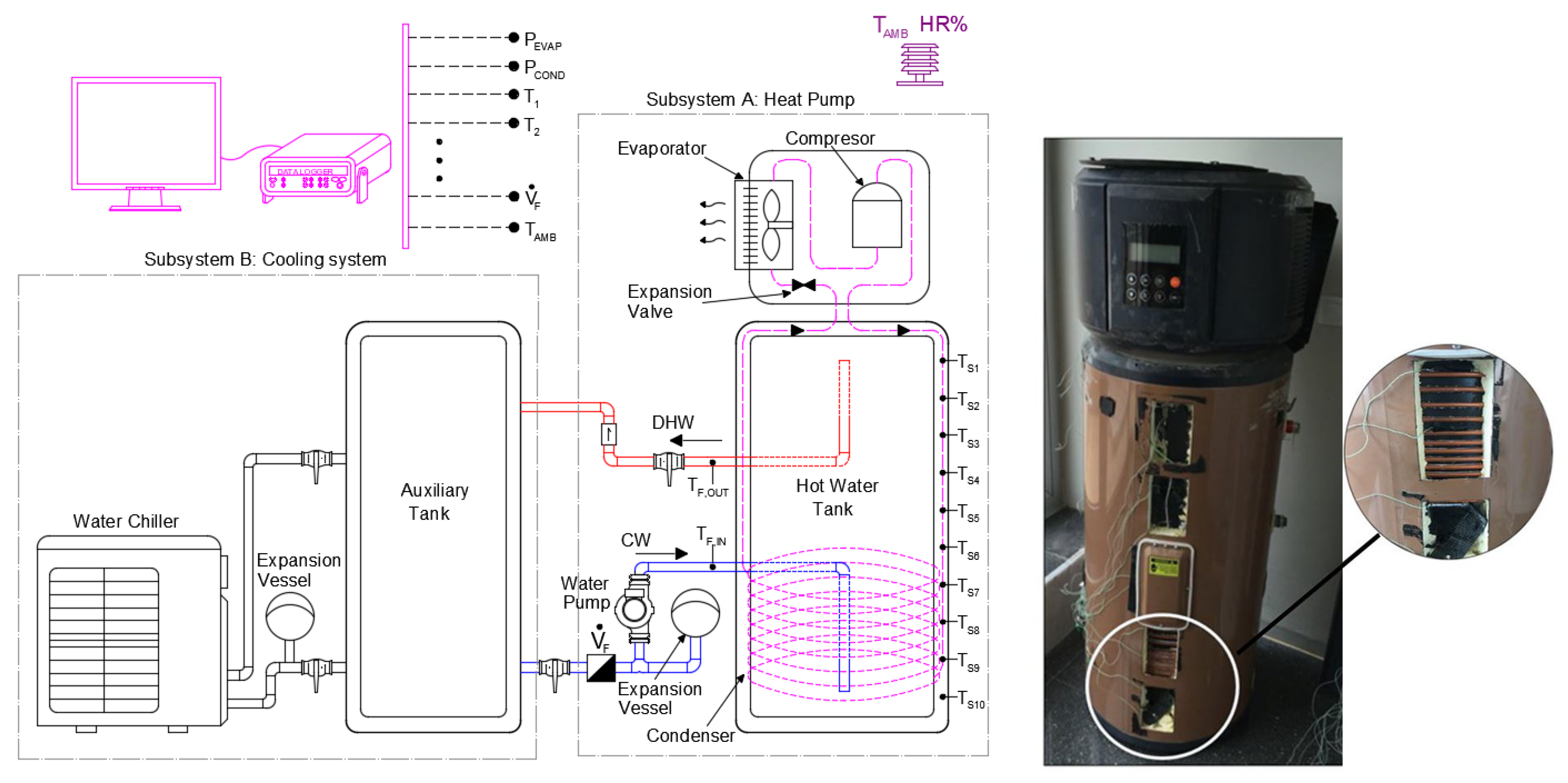
The test facility scheme is shown in Figure 1, where the tested DHW heat pump system (subsystem A), the consumption simulation system (subsystem B), and all the gauges and sensors used (temperatures, flow, consumption, etc.) are included. In addition, since the experimental set-up is located outdoors, a meteorological station was installed to monitor working conditions (temperature, humidity, wind, and solar radiation).

In subsystem A, the hot water tank has a capacity of 190 L ($Ø0.47$ m × $1.1$ m). The tank wall is made of 3 mm thick steel ($k=50$ W/mK), with a 45 mm thick external insulation layer ($k=0.04$ W/mK) protected by an aluminium film. The refrigerant cycle’s condenser coil is made of a 6 mm copper tube that loops 15 times and wraps around the outside of the bottom of the tank. A series of gauges was installed to measure, among other things, the tank inlet and outlet water temperatures and flow rate during tapping. Likewise, a total of 10 thermocouple temperature gauges were placed vertically along the tank’s metallic body on the outer wall. Figure 1 (right) shows the sensor’s installation process and a schematic representation of the sensor’s positioning. (Insulation is set back once the sensors are placed in order to prevent heat losses.) Power consumption was measured with a network analyser Chauvin Arnoux CA8332B.

Subsystem B is mainly composed of an ON/OFF water chiller and an auxiliary water tank of 200 L as well as an expansion vessel. The aim of this subsystem is to chill and store the water that has previously been heated by the heat pump. Both systems are connected by a closed loop circuit which also includes a centrifugal pump, a Siemens MAG 1100 F flow meter and an expansion vessel. This configuration allows testing to avoid waste of water. Data were recorded uninterruptedly by an HP Agilent 34,970 A data acquisition system. A programmable control system governs the heat pump’s starting and stopping times, the DHW consumption timetables, regulation and control, etc.

3. Tank Stratification Experimental Results

In order to carry out an energetic analysis of the heat pump and the water stratification inside the tank, a series of experimental tests were carried out.

For that purpose, three experimental tapping cycles were designed to observe the heat pump performance and water stratification inside the tank in the context of hot water consumption in dwellings. The design of the experiments is mainly based on the curves S and M of the international standard, [28] in terms working conditions, of energetic daily consumption, flow rate, and both on the standard and the data reported by [29] in terms of the consumption timetable. The Standard [28] describes the specific methods and conditions for testing heat pumps with electrically driven compressors connected to or including a domestic hot water storage tank.

Each tapping was programmed to last 5:30 min, following the tapping cycles shown in

Table 2. Consumption timetable for the designed tapping cycles.

Tapping Cycle	Flow Rate	7:00	8:00	9:00	13:00	19:15	20:15	Total (Litres)
TC1—6 × 22 L	4 L/min	22 L	22 L	22 L	22 L	22 L	22 L	132 L
TC2—6 × 33 L	6 L/min	33 L	33 L	33 L	33 L	33 L	33 L	198 L
TC3—3 × 33 L	6 L/min	-	33 L	-	33 L	33 L	-	99 L

. In each experiment, the heat pump is activated at 11:00 a.m. and turns off when the water reaches 55 $°$C (temperature sensor is at the bottom 1/4 height inside the tank). All the experiments were carried out for an inlet water temperature of 15 $°$C and under real external conditions. The ambient temperature was between 19 $°$C and 23 $°$C during the working time of the heat pump.

Table 3. Tank stratification experiments. Measurements taken and recorded every minute.

Description	Unit	Symbol	Accuracy
Inlet water temperature	$°$C	$T_{F,IN}$	$\pm 0.05°$C
Outlet water temperature	$°$C	$T_{F,OUT}$	$\pm 0.05°$C
Water flow rate	L/h	${\dot{V}}_F$	$\pm 1$% R.D.
Refrigerant temp. in the compressor’s inlet	$°$C	$T_1$	$\pm 1.5°$C
Refrigerant temp. in the compressor’s outlet	$°$C	$T_2$	$\pm 1.5°$C
Refrigerant temp. in the condenser’s outlet	$°$C	$T_3$	$\pm 1.5°$C
Refrigerant temp. in the evaporator’s inlet	$°$C	$T_4$	$\pm 1.5°$C
Refrigerant condensing pressure	bar	$p_C$	$\pm 0.17$%
Refrigerant evaporating pressure	bar	$p_E$	$\pm 0.14$%
Power consumption of the heat pump	W	$P_{HP}$	$\pm 0.5$%
Temperature on the surface of the tank	$°$C	$T_{F,s_1}$…$T_{F,s_{10}}$	$\pm 1.5°$C
External ambient temperature	$°$C	$T_{AMB}$	$\pm 0.3°$C

shows the parameters, which were recorded every minute. These measurements allowed us to carry out an energetic analysis of the heat pump and the water stratification inside the tank.

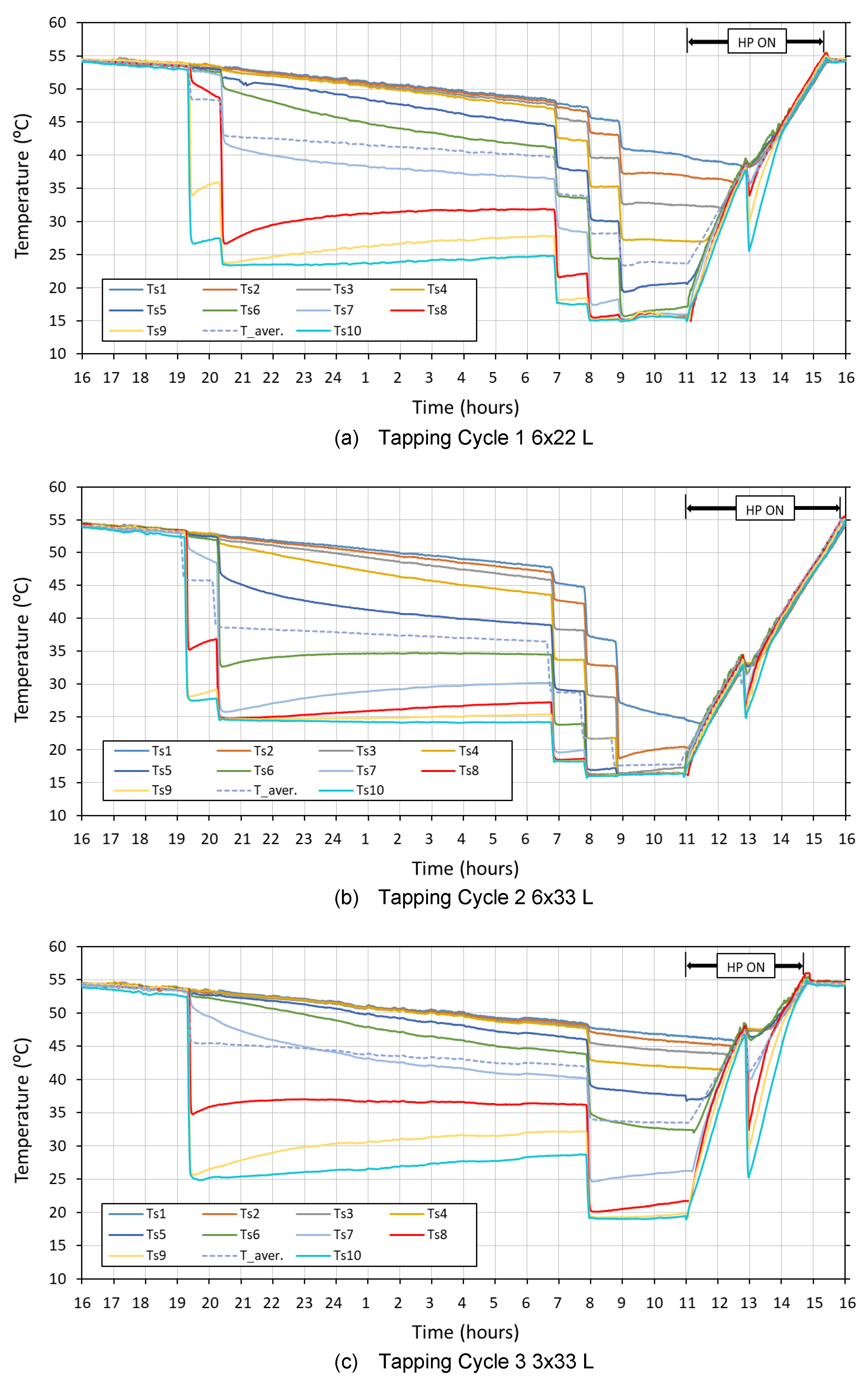
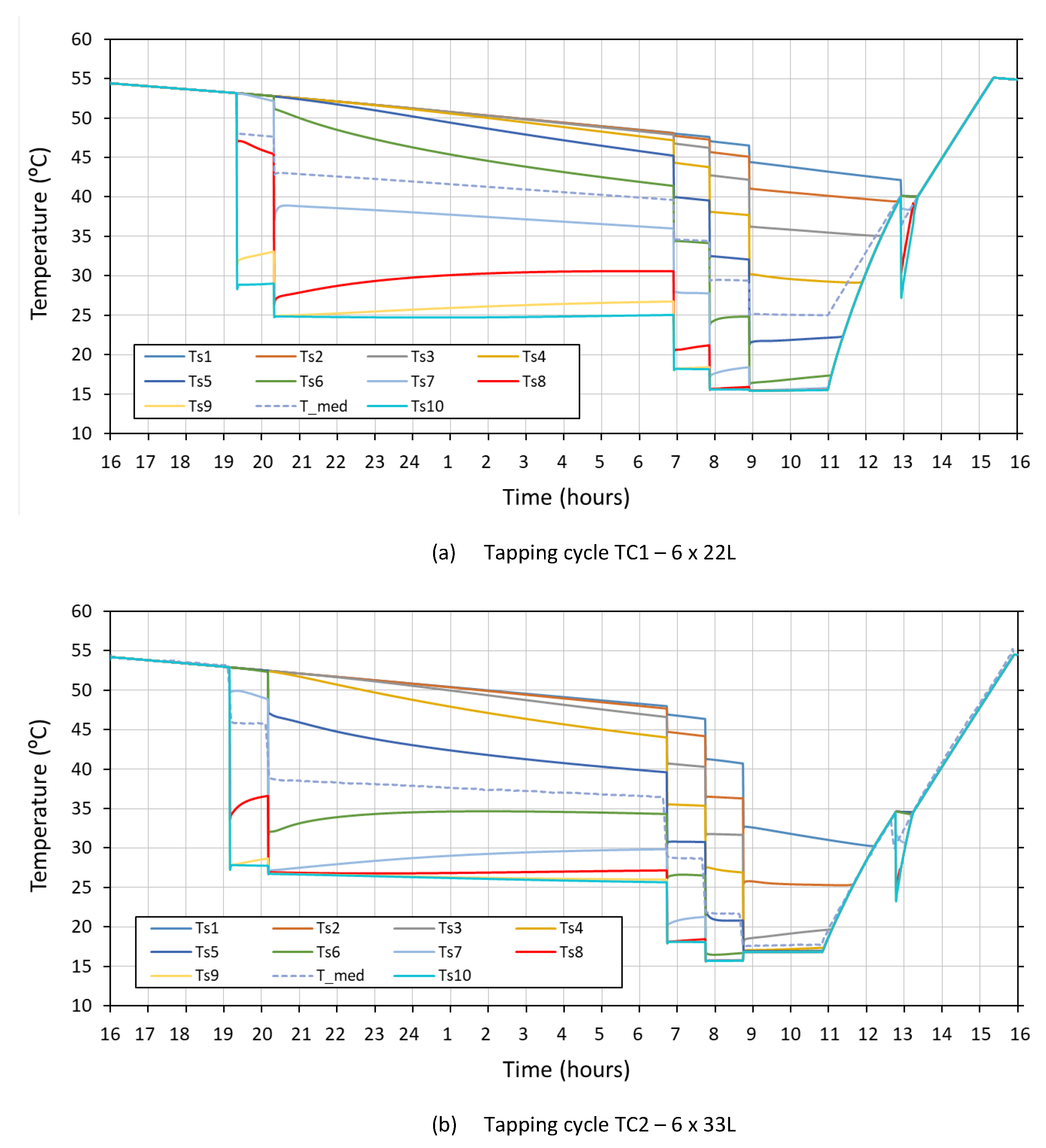
Figure 2 shows the evolution of the 10 temperatures on the surface of the tank, from (sensors $T_{s1}$ to $T_{s10}$ of Figure 1), during each experimental tapping cycle analyzed. To clarify the figure, the temperatures were plotted from 16 p.m. to 16 p.m. of the next day, because that was when the water temperatures were homogeneous at 55 $°$C. While the tank was fully charged, it was at a uniform temperature. As the tank cooled due only to heat losses (16–19 h), the effect of stratification, though present, was negligible for this period of time.

In all the experiments, after the first DHW consumption, only the three bottom sensors ($T_{F,s_8}$ to $T_{F,s_{10}}$ at Figure 1) register a significant drop in temperature. At this point, the tank is rather heavily stratified, showing significant temperature differences between the cool section at the bottom part and the hot section at the top. In addition, the post-draw water temperature at the lowest tank region was above that of the inlet water ($T_{F,IN}=15°$C). This shows that tank water had been mixed with inlet water during the water draw.

After each consecutive consumption, the tank became more and more stratified as its thermocline region crept upwards and became taller. For example, during the first draw in the TC1 experiment, sensor $T_{F,s_6}$ registered no significant temperature variation, yet after the second simulated consumption, the same sensor registered a temperature drop of 2.5 $°$C. Sensor $T_{F,s_4}$ experienced no significant temperature drops until draw 3, while sensor $T_{F,s_1}$ registered its first significant temperature drop after the fifth draw.

Another phenomenon that can be observed is that regions at the bottom of the tank tended to reheat through heat conduction in the vertical direction after the initial consumption-induced temperature drop. A similar but mirrored effect was consequently observed in the water regions directly above. At 11:00, the heat pump was activated, and the tank water began to heat up. It becomes apparent that while the heat pump was on, the tank heated up from the bottom upwards. As the heat pump was engaged in the stratified tank, it had little or no effect on the upper, warmer regions. Water at any given level did not begin to heat up until regions below it had reached its temperature. In fact, during the initial stages of the heat pump’s activation, water regions at the top of the tank continued to cool down.

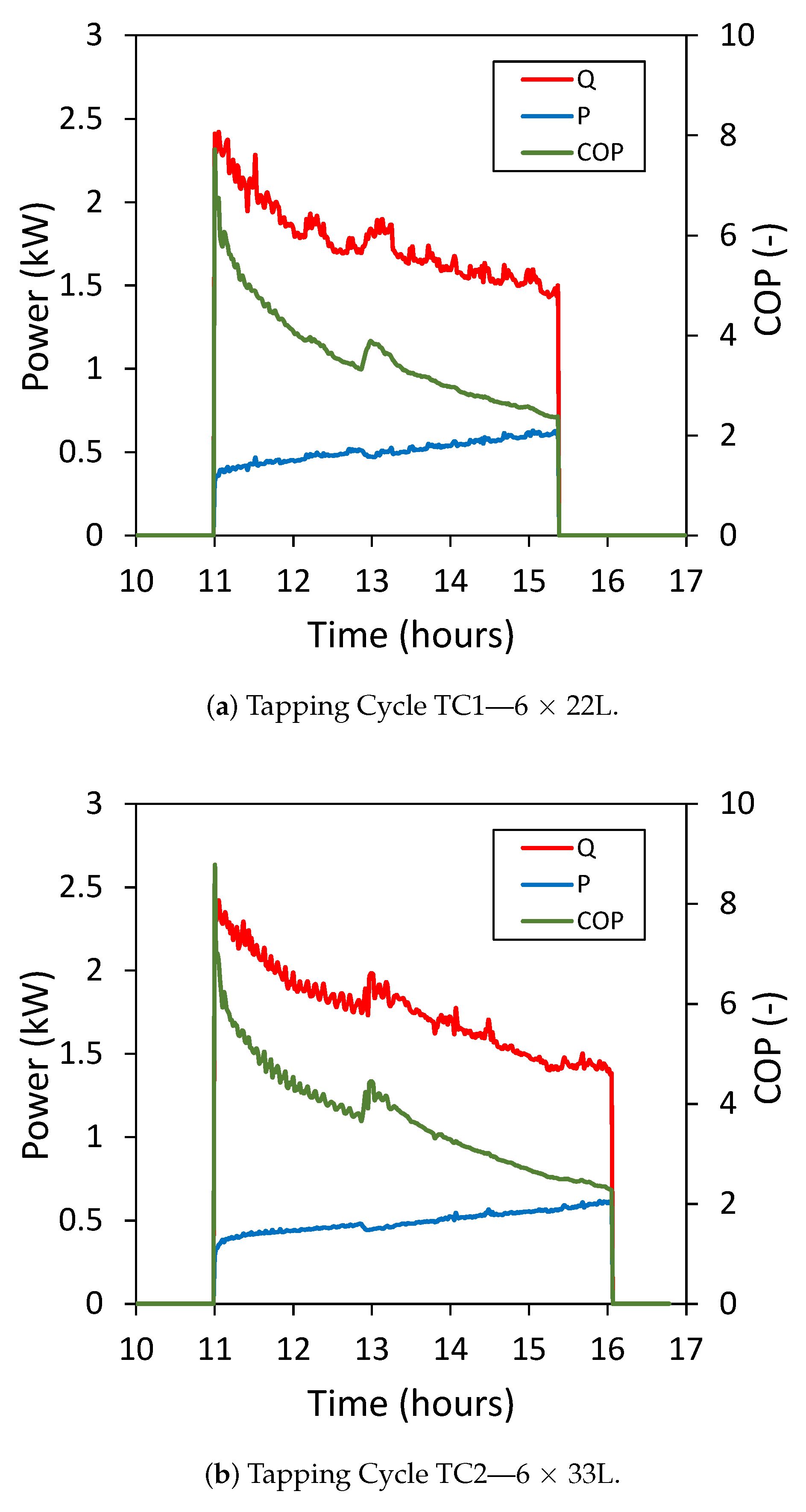
The useful heat provided to the water by the condenser ($Q_{HP}$) and the electric power consumption by the heat pump ($P_{HP}$) were obtained by using the methodology described in [4]. Both parameters and their ratio, the $CO{P}_{HP}$, are plotted at Figure 3 for the tapping cycles TC1 and TC2. The results show that as the water temperature at the condenser level ($T_{F,s_7}$ to $T_{F,s_{10}}$) increases, so does the electrical consumption while the useful heat decreases, decreasing as a result the $CO{P}_{HP}$ of the heat pump. In addition, it can be observed as the engagement time of the heat pump is longer in the TC2 than in the TC1 tests. The reason is that water consumption in TC2 is 66 L higher than in TC1. Therefore, the water tank reaches a lower temperature in TC2, and the heat pump takes longer to heat it up back to 55 $°$C.

Table 4. Heat pump performance during tank stratification experimental results for tapping cycles TC1, TC2, and TC3.

Tapping Cycle	${\mathit{Q}}_{\mathit{HP}}$	${\mathit{E}}_{\mathit{HP}}$	${\mathit{COP}}_{\mathit{HP}}$	${\mathit{T}}_{\mathit{AMB}}$	${\mathit{T}}_{\mathit{f},{\mathit{s}}_{7-10}}$	Working Time
	kWh	kWh	-	$°$C	$°$C	h
TC1—6 × 22 L	7.71	2.22	3.47	22.6	34.8	4.38
TC2—6 × 33 L	8.89	2.50	3.55	19.1	31.2	5.07
TC3—3 × 33 L	6.18	1.96	3.15	20.5	38.9	3.8

shows a summary of the main energetic parameters of the three tapping cycles experiments.

The experimental results in this section were used for the development, adjustment, and validation of the numerical model, which is described next.

4. Numerical Model of the Domestic Hot Water Heat Pump

A computational model for the simulation of the heat pump water heater system (HPWH) behavior was implemented in Matlab. The model was built in two steps.

Firstly, a numerical model of the hot water tank has been developed. Thanks to this model, the water temperature at the bottom part of the tank, where the condenser is located, could be obtained. Secondly, an analytical model of the refrigeration cycle was defined. Both models were validated using the experimental results detailed in Section 3, and the one-year experimental results described in [4].

4.1. Numerical Model of the Tank

The experimental data revealed the process physical difficulties and implications regarding the flow behavior inside the hot water tank. They also served to determine fundamental needs of the model to be put in place. As stated before, the mechanism governing the fluid behavior most of the time was very simplistic, as convection is negligible and heat transfer is mainly due to conduction. However, the fluid behavior gets more complicated during and immediately after water draws, when convection becomes significant and is influenced by a number of factors. A numerical model was created to evaluate the energy equation along the vertical axis, with the following assumptions:

• One-dimensional heat conduction in the fluid and in the tank wall: Temperature variation within the fluid and tank wall only occurs along the vertical axis ($\partial T_F/\partial r=0$ and $\partial T_F/\partial \theta =0$).
• The water inlet is at the bottom part of the tank and the outlet at the upper one.
• The condenser coil is at the bottom of the tank.
• Insulation is equally distributed around the surface of the tank.
• The transport phenomena, which is important only during short periods of time, has been considered by using the experimental correlations described in Section 4.1.1.
• Heat flux from the heat pump is modeled as a uniform heat flux at the tank wall surface at the location of the condenser coil.

With the former considerations, the energy equation is uncoupled from the momentum equation and results in

$$\rho C_P\frac{\partial T}{\partial t}=\dot{q}+k\left(\frac{{\partial }^{2}T}{\partial z^2}\right)$$

(1)

The one-dimensional multinode model was discretized into finite volumes, as shown at Figure 4. Thus, the energy equation for the fluid inside the tank and for the tank wall result in:

$${\rho }_F{V}_F{C}_{P,F}\frac{T_{F_n}^i-T_{F_n}^{i-1}}{\Delta t}={\dot{Q}}_{W{F}_n}^i-k_F{A}_F\left(\frac{T_{F_{n+1}}^i-2T_{F_n}^i+T_{F_{n-1}}^i}{\Delta z}\right)$$

(2)

$${\rho }_W{V}_W{C}_{P,W}\frac{T_{W_n}^i-T_{W_n}^{i-1}}{\Delta t}={\dot{Q}}_{W{F}_n}^i-{\dot{Q}}_{W{F}_n}^i-{\dot{Q}}_{L_n}^i-k_W{A}_W\left(\frac{T_{W_{n+1}}^i-2T_{W_n}^i+T_{W_{n-1}}^i}{\Delta z}\right)$$

(3)

The heat generated by the heat pump is defined as ${\dot{Q}}_{HP}$. This heat, generated in the condenser coil that surrounds the bottom quarter of the tank wall, is modeled as generation in the tank wall. The boundary conditions are the heat losses ${\dot{Q}}_L$ and the thermal flux from the tank wall to the fluid ${\dot{Q}}_{WF}$.

$${\dot{Q}}_L=h_{WE}{A}_{WE}(T_W-T_{AMB})$$

(4)

where the coefficient $h_{WE}$ is calculated from specific experimental measurements carried out in the tank, which allowed us to estimate its losses. That tests started with an homogeneous temperature within the tank of 55 $°$C and was left to cool down for 72 h. Finally, a value of $h_{WE}=2.2$ W/$°$C was obtained.

$${\dot{Q}}_{WF}=h_{WF}{A}_{WF}(T_W-T_F)$$

(5)

The thermo-physical properties of the fluid were considered constant and uniform within the model (${\rho }_F=1000$ kg/m${}^3$, $C_{P,F}=4180$ J/kg$°$C, and $k_F=0.6$ W/m$°$C). Similarly, the model uses the following thermo-physical properties for the steel tank wall: ${\rho }_F=8000$ kg/m${}^3$, $C_{P,F}=466$ J/kg$°$C, and $k_F=50$ W/m$°$C.

After a study of the mesh convergence, it was found that, by dividing the tank into 100 layers and iterating over 1 min timesteps, the solution converged, showing a deviation in comparison to the the solution with 500 layers lower than 0.1% (in terms of energy and temperatures).

4.1.1. Tank Model Transport Phenomena

The numerical model is based on the analysis of the energy equation without considering the convective term. To overcome that, the numerical model is complemented by a set of empirical equations that consider the effects of convection in the following two cases:

• Flow mixing during water draws. During DHW consumption, the inlet jet that enters the tank mixes with the bottom tank water.
• Natural convection. When water is heated at the bottom of the tank, buoyancy forces caused by thermal differences between fluid layers produce natural convection.

Firstly, the flow mixing that occurs during water draws is addressed. Although tank up-flow is not considered to produce significant mixing, the literature review [7] and the experimental results prove that mixing due to the water inlet is a highly influential destratifying factor. Literature suggests that several factors impact mixing due to inlet flows, such as inlet velocity and inlet configuration. Thus, the higher the inlet velocity, the greater the mixing is.

Another factor that significantly impacts destratification is the temperature difference between the inlet water and the local tank water into which the inlet water is being injected. The mixed volume of hot water inside the tank depends on the relation between the inertial forces and the buoyancy forces. If the temperature difference is low, buoyancy forces are not important and the inertial forces due to the inlet water are dominant. This results in a big mixed volume of the hot water in the tank (significant destratification). On the contrary, if the temperature difference is high, buoyancy forces are dominant, and only a small volume of water gets mixed.

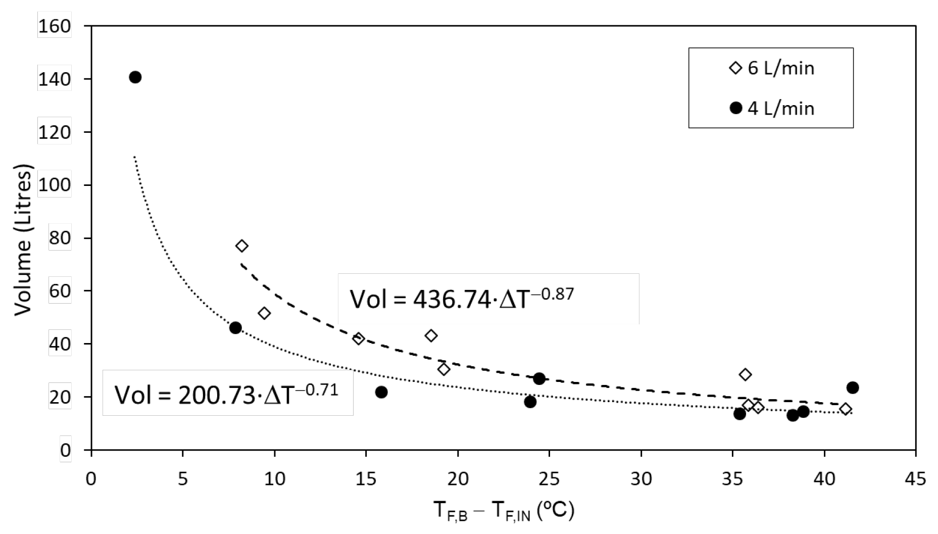
In order to incorporate this behavior into the model, results from the experimental phase of the research were re-analyzed with the specific goal of finding a relationship between relative inlet temperatures and tank mixing. The aim is to determine the volume of water that is affected by the mixing mechanism, $V_{MIX}$.

Given that inlet velocity also has a great effect on this mechanism, the experimental results were carried out for two flow rates: 4 L/min and 6 L/min. Measurement results are shown at Figure 5. For each group, a mixing empirical equation has been obtained:

$$V_{MIX}=200.73\Delta T_{F,B-F,IN}^{-0.71},\mathrm{for}{q}_{IN}=4\mathrm{L}/\min$$

(6)

$$V_{MIX}=436.74\Delta T_{F,B-F,IN}^{-0,87},\mathrm{for}{q}_{IN}=6\mathrm{L}/\min$$

(7)

where $\Delta T_{F,B-F,IN}$ is the temperature difference between the inlet fluid and the fluid at the bottom of the tank before the water consumption. The constants in Equations (6) and (7) are defined for a volume in liters and a temperature difference in Kelvin or Celsius degrees.

These equations are used in the model to find the number of layers that mix with the incoming mains water.

Secondly the natural convection mechanism inside the tank is addressed. In a stratified tank, the temperature gradient in the vertical direction (upwards) is null or positive. However, when water is heated at the bottom of the tank, the buoyancy forces caused by thermal differences between fluid layers produce natural convection.

The experimental results indicate that there is no intense flotation effect that causes water to “shoot up” the tank, thus causing a significant current and hence inducing mixing. The warmed water simply floats up the regions immediately above it, as its density fluctuation does not allow it to remain near the heat source long enough to experience a high density change. Instead, the floating effect simply limits regional temperatures, so that each region is never warmer than the one above it.

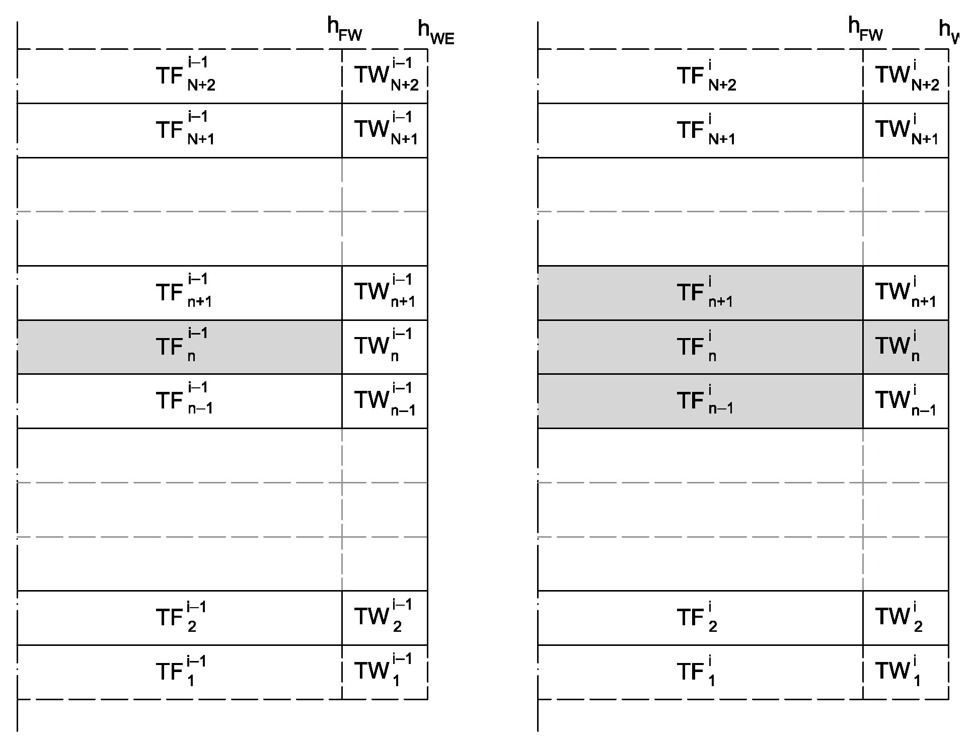
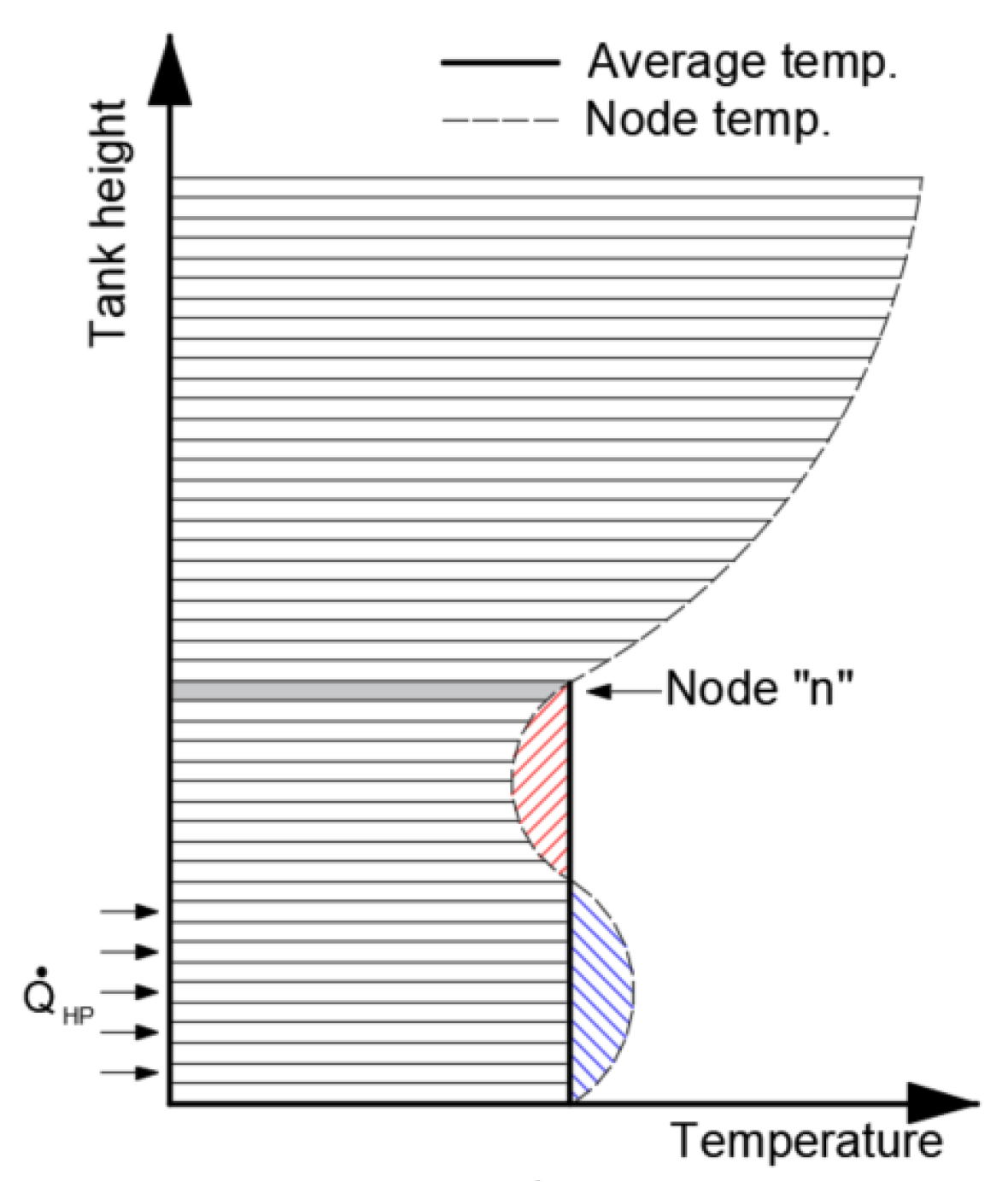
For the modelization of convection, the first step is to find the lowest control volume (CV) that is warmer than the average temperature of that CV and the ones below it (Figure 6). Then, the temperatures of all that layers are set to their average temperature in order to create a new uniform temperature profile.

The great advantage of the method described above is its extreme computational efficiency, as it requires only a few iterations. The solution also accounts for the mixing effects of the rising plume. As can be seen in Figure 6, the layers directly above the warm region are heated, while the lower, warmer region is cooled. The algorithm essentially redistributes energy without altering the total energy content of the affected layers.

This natural convection algorithm is applied once every time step (1 min) only when the heat pump is working.

4.2. Validation of the Tank Model

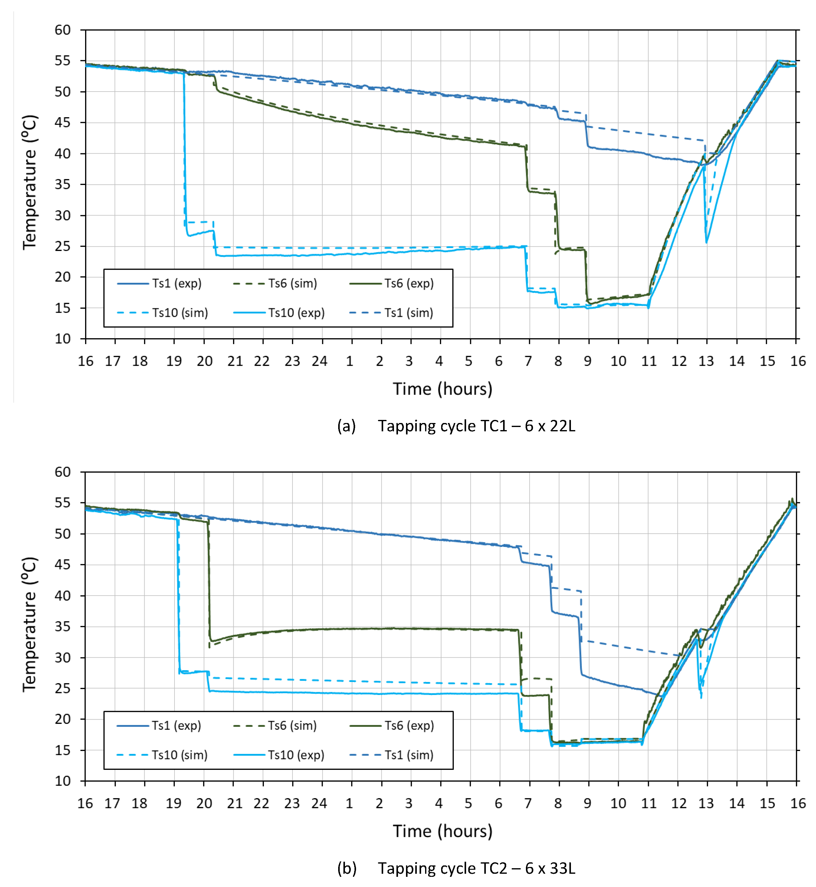
Figure 7 show the numerical results of the tank stratification for two tapping cycles TC1 and TC2. The results display the same general shape and exhibit the same characteristic features and tendencies as experimental data. For instance, even after various consumptions were replicated, both simulated and experimental data show that temperature evolution at the top of the tank was largely unaffected by inlet water.

A key advantage of stratification within the heat pump hot water heater is that the lower layers of the tank, where the condenser coil is located, tend to be cooler than they would be in a fully mixed tank. This not only increases the temperature gradient and thus aids heat transfer, it also increases the heat pump COP. It is thus highly important that the model is capable of replicating stratification and the temperature evolution in the tank, in order to properly reflect this advantageous behaviour.

A comparison between experimental and numerical results was carried out for the taping cycles TC1 to TC3, showing an error of 2.6 $°$C (95% confidence level) in the tank water temperature at the condenser location when the heat pump was working. Figure 8 shows such a comparison for TC1 and TC2 cycles. For greater clarity, only one representative sensor from each tank region is plotted: $T_{F,s_1}$, $T_{F,s_6}$, and $T_{F,s_{10}}$ for upper, middle, and low tank regions. As can be observed, the numerical results match the experimental ones closely throughout the day. Nonetheless, significant differences are observed between simulation and experimental results for $T_{s_1}$ when its value falls below $45°$C, but this situation does not occur in standard operation conditions, where a minimum hot water supply temperature must be ensured. Consequently, the validity of the model for the simulation of a plethora of scenarios with accuracy and reliability has been demonstrated. Furthermore, the results show that the model succeeds in simulating the three physical phenomena that interpose in the tank’s energy balance equations:

• Mixing that occurred during DHW consumption (experimentally modeled by Equations (6) and (7)).
• Heat conduction between regions while the tank is stratified (see temperatures between 21:00 and 6:00 in Figure 8).
• The natural convection mechanism.

4.3. Analytical Model of the Refrigerant Cycle

The heat pump water heater under study was tested for a typical DHW production of a four-member dwelling in Spain with a water consumption around 130 L per day at 55 $°$C (about 6.2 kWh/day). This project, described in-depth by the authors in [4], was carried out during more than 240 days in order to establish seasonal results. Now, some of those measurements have been used to develop the analytical model described in this section, which is capable of simulating the heat pump behavior under different working conditions.

For that purpose, a data selection and filtering process was carried out from the experimental results in order to narrow down to working points in stationary conditions and with the heat pump in operation. Thus, 10 to 15 working points for each day were found valid.

As a result, a total of more than 300 valid points were selected from the annual project, which comprise different outdoor and tank temperatures. The results in steady conditions were joined and collected in order to set an analytical model for the heat pump, based on the model of electrical heat pump equations proposed by the building energy analysis program DOE-2.

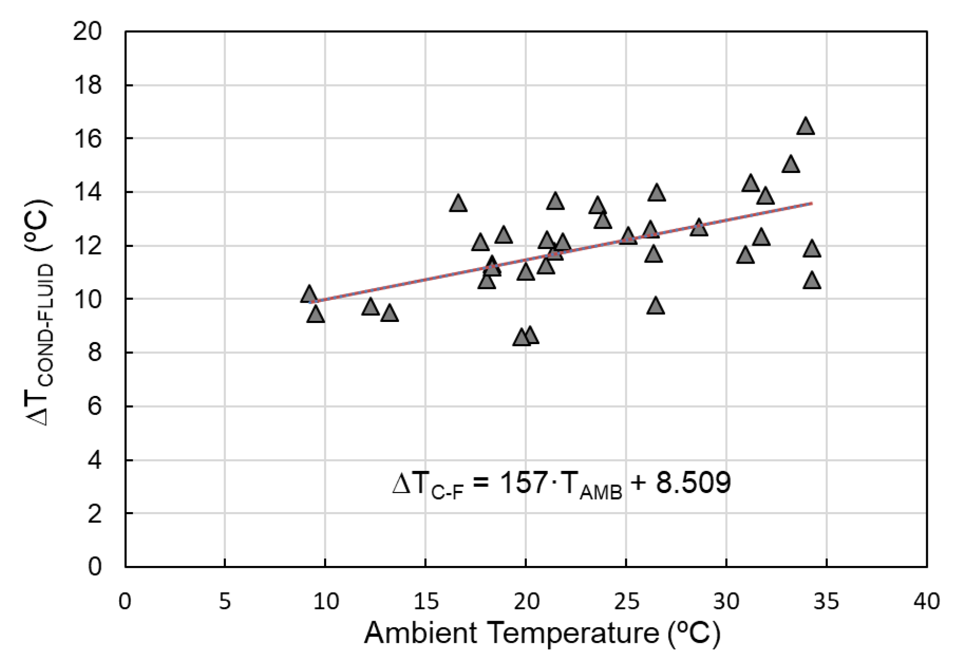
The dependencies between the different variables were analyzed. Thus, it has been stated that the evaporator ($T_E$) and condenser temperatures ($T_C$) are the main variables impacting both the electrical power consumption ($P_{HP}$) and the useful thermal power supplied by the heat pump to the water ($Q_{HP}$). In addition, both temperatures depend on the tank water temperature ($T_F$) at the coil position (see Figure 9) and the outdoor ambient temperature ($T_{AMB}$).

Experimental correlations between the former variables are presented next:

$$\Delta T_{C-F}=8.509+0.157T_{AMB}$$

(8)

$$T_E=-14.46+0.645T_{AMB}+0.230T_F$$

(9)

$$\begin{array}{cc}\hfill {\dot{Q}}_{HP}=& 3434.7+106.5T_E-66.4T_C+\hfill \\ & +0.766T_E^2+0.410T_C^2-1.026T_E{T}_C\hfill \end{array}$$

(10)

$${\dot{P}}_{HP}=310.7-0.097T_E^2+0.510T_C^2+0.097T_E{T}_C$$

(11)

The heat pump instantaneous coefficient of performance can be obtained as the ratio between the heat flux and the heat pump consumption:

$$CO{P}_{HP}=\frac{{\dot{Q}}_{HP}}{{\dot{P}}_{E,HP}}$$

(12)

4.4. Refrigerant Cycle Model Validation

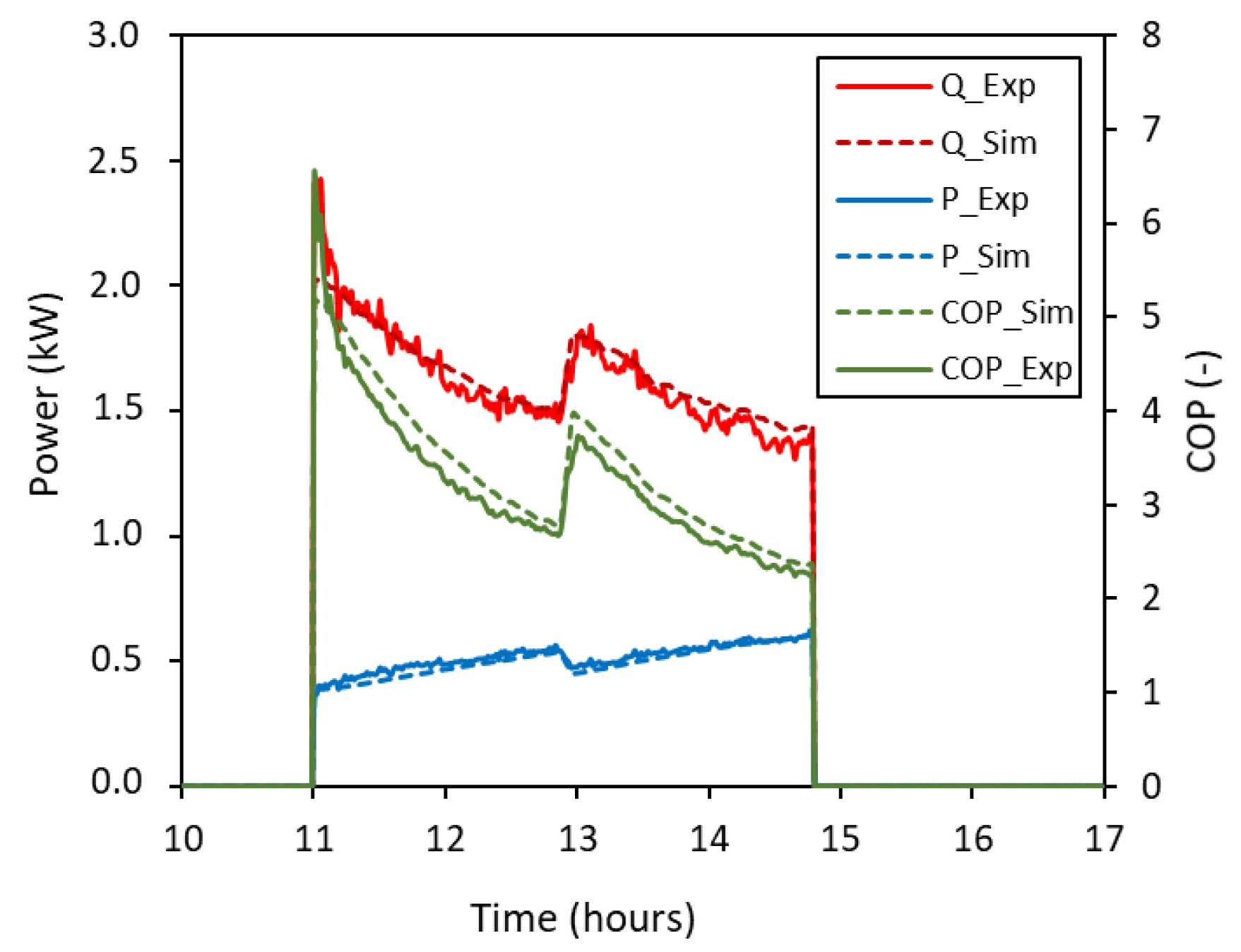
In order to validate the analytical model described in Section 4.3, the obtained equations were applied to several days of experimental work using the following input data: the water temperatures at the bottom of the tank ($T_F$) and the outdoor ambient temperature ($T_{AMB}$). Figure 10 shows a comparison of the experimental and simulation results of the energy analysis for the TC3 test, described in Section 3. In the figure, the thermal power (${\dot{Q}}_{HP}$), the power consumption ($P_{HP}$), and the heat pump efficiency ($COP$) are plotted for the test.

It can be observed that the simulation curves are quite similar to the experimental ones for all the parameters under comparison. The high accuracy reached for the power consumption estimation has to be highlighted, where the curves are almost equal. Energy results for the analyzed days show a deviation between experimental and simulation results of only 5.1% for the COP for 95% of confidence level. Therefore, it can be concluded that the analytical model has been successfully validated.

5. Application of the Model to Standard 16147

As was introduced previously, the standard [28] describes the specific methods and conditions for testing heat pumps with electrically driven compressors connected to or including a domestic hot water storage tank. A total of ten tapping cycles are described in the standard, corresponding to different quantities of hot water preparation energy consumption per day, ranging from the 3XS ($0.345$ kWh/day) to the 4XL ($93.520$ kWh/day). The tapping cycles are designed in an effort to reproduce the typical consumption occurring in the residential and commercial sectors. The standard describes tests for different temperatures of the air inlet to the evaporator ranging from $2°$C to $20°$C. For all of them, water inlet temperature is 10 $°$C and water preparation temperature is 55 $°$C, while the temperature around the hot water tank is of 20 $°$C.

The coefficient of performance for the full tapping cycle (24 h) can be obtained as:

$$CO{P}_{DHW}=\frac{Q_{DHW}}{E_{HP}}$$

(13)

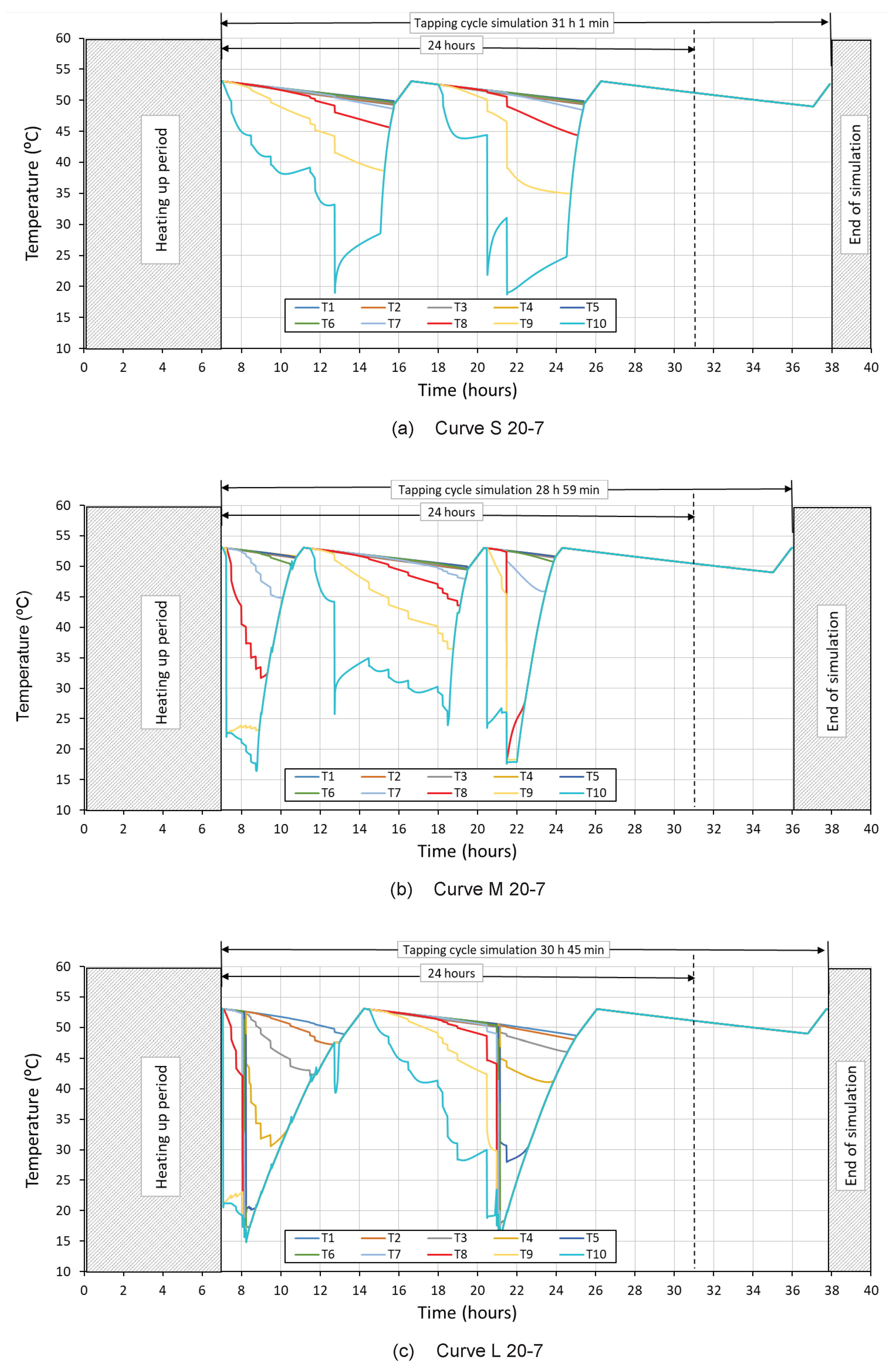
In this work, the developed numerical model has been employed to simulate the testing procedure of a heat pump water heater according to Standard EN 16147. Reference tapping cycles S, M, and L (typical of family dwellings) at two outside temperatures, 7 $°$C and 20 $°$C have been simulated.

The starting time and hourly energy consumption for the three curves are detailed in the Standard. For example, the M curve includes 23 DHW consumptions per day. This represents the typical consumption in a family dwelling: 19 small ones of 0.105 kWh, 2 for showers of 1.4 kWh, and 2 for dish washing machine of 0.315 kWh and 0.735 kWh. The previous results in a total thermal energy consumption of 5.845 kWh/day. It should be noted that this amount of energy does not include tank heat losses.

Figure 11 shows the temperature stratification evolution within the DHW tank, along the simulation for the S, M and L reference tapping cycles, where the inlet water temperature is 10 $°$C for all the tappings and the tank ambient temperature is 20 $°$C. Simulations have been carried out for air inlet temperature to the evaporator of 7 $°$C (20/7) and 20 $°$C (20/20). As before, $T_{F,s_1}$ corresponds to the temperature in the upper part of the tank and $T_{F,s_{10}}$ in the lower part.

Energy and performance simulation results are shown at

Table 5. EN 16147 simulated results of reference tapping cycles from S, M, and L. Energy and performance results for an ambient temperature of 20 $°$C and inlet air temperatures to the evaporator of 7 $°$C and 20 $°$C.

Variable	Uts.	S (20/20)	M (20/20)	L(20/20)	S (20/7)	M (20/7)	L (20/7)
$Q_{DHW}$	kWh	2.03	5.80	11.56	2.03	5.82	11.48
$Q_L$	kWh	2.49	2.31	2.26	2.57	2.38	2.34
$Q_{HP}$	kWh	4.52	8.11	13.82	4.60	8.20	13.82
$E_{HP}$	kWh	1.50	2.61	4.21	2.02	3.48	5.46
$CO{P}_{DHW}$	-	1.4	2.2	2.7	1.0	1.7	2.1
$CO{P}_{HP}$	-	3.0	3.1	3.3	2.3	2.4	2.5
$T_{f,s_{7-10}}$	$°$C	50.0	49.0	47.5	49.8	48.5	45.4

. According to the simulations for the six reference tapping cycles established at EN 16147, the $CO{P}_{HP}$ of the heat pump, calculated as the ratio of supplied thermal energy and electrical energy consumption, varies between 2.79 and 3.24 when the air supplied to the heat pump is 20 $°$C and between 2.11 and 2.49 at 7 $°$C. Both the effects of the external temperature and the tank temperature are important (Tapping cycle L produces a lower temperature in the tank than Tapping Cycle S). As shown by the results, for the same simulation conditions (20/20 or 20/7), the lower the tank water temperature at the coil ($T_{f,s_{7-10}}$), the greater the $CO{P}_{HP}$. However, according to the Standard, only the DHW useful thermal energy must be used in the calculation, resulting in very different $CO{P}_{DHW}$ depending on the DHW consumption. In fact, it can reach values from $CO{P}_{DHW}$ = 1.04 for Cycle S (20/7) to 2.76 for Cycle L (20/20).

6. Conclusions

The main objective of this work was to develop a model of a compact DHW heat pump, as well as to carry out experimental tests for the calibration and validation of the model. The novelty of this work lies mainly in the following two points. Firstly, it is a smart model with low computational cost requirements. Secondly, manufacturers could apply this model to their heat pumps, for which only a few simple experimental tests are required in order to adjust the model. (A new adjustment of the model would be required for a different device or consumption flow rates.) Once it is adjusted, it could be used to determine the performance of the heat pumps under different working conditions (tapping cycles, operation temperatures, …) quickly and straightforwardly, without complex and extensive experimental tests.

• A numerical model of a tank integrated heat pump for Domestic Hot Water production has been developed and experimentally adjusted and validated. The model accurately simulates the heavily stratified tank after several water draws and the water heating process. The computational cost of long-term simulations is low, which allows it to be used even in one year simulations (a 365 days simulation takes less than 5 h with a standard personal computer).
• The tank model uses experimental correlations to account for the complex flow mixing mechanism during water draws at 4 and 6 L/min. The numerical model simulates properly natural convection inside the water tank during and after water draws and the water heating process. It has also been proved to mimic the temperature stratification within the hot water tank with significant accuracy (deviation of 2.6 $°$C for a 95% confidence level), when using several tapping cycles and flow rates, thus providing versatility and reliability.
• The model was demonstrated to be reliable when determining the useful thermal power supply from the condenser to the water, the electrical power consumption, and the COP of the heat pump. Energy results for the analyzed days show a deviation between experimental and simulation results of only 5.1% for the COP for a 95% confidence level.
• Finally, the computational model was used to simulate six reference tapping cycles from the Standard EN 16147: tapping cycles S, M, and L, at air inlet temperatures of 20 $°$C and 7 $°$C. These results show a practical application of the model where manufacturers can see the potential of simulation models.

As mentioned before, there is a wide range of potential applications for this model. It can be used in engineering design to reveal influences of control strategies and component sizing. For example, with the objective of increasing the photovoltaic self consumption in dwellings, heat pump water heaters can be designed for this purpose.