1. Introduction
Global market competition and an increase in customers’ demands have caused global supply chains to become larger networks [
1]. The members of global supply chains include production companies (final assemblers, suppliers) and service providers. The most important service providers are the transport companies [
2,
3]. Therefore, the optimization of transport activities’ fuel supply and the minimization of the transport costs are relevant issues to address, particularly in consideration of the COVID-19 pandemic. The motivation behind and significance of our research are detailed here:
Transport companies had thus far not applied a mathematical method to address drivers’ ad-hoc decision-making and, in not doing so, had encountered financial and time losses. Based on this issue, we sought to create a new decision-supporting cost optimization method for fuel supply optimization for drivers and their transport trips. Consequently, our research topic is timely and important.
As mentioned, the primary aim of our research is to develop a new optimization method for the minimization of road freight transport costs in order to reduce the fuel costs and, correspondingly, determine the optimal filling stations and to calculate the optimal quantity of fuel for refueling. The optimization method we developed features two phases and addressed two main research questions:
In the first phase, the optimal, most cost-effective fuel station is determined based on the zone of potential fuel stations. The zone of these stations refers to the area where drivers have to refill their vehicles before the fuel level becomes critical, i.e., low and nearing ‘empty’. Specific fuel prices differ per potential fuel station, and the stations are located at different distances from the main transport way. The method we developed can support drivers’ decision-making regarding the optimal fuel station, i.e., the most cost-effective fuel station, taking into consideration both the specific fuel prices and the additional transport distances. The method can guide drivers’ decision to refuel at a farther but cheaper fuel station or at a nearer but more expensive fuel station based on which choice is more economical.
In the second phase, the optimal volume of the fuel is determined, i.e., the exact volume of fuel required, including a safe amount to cover stochastic incidents (e.g., plus consumption due to road closures or accidents etc.). The optimal amount of fuel relates to the volume necessary for the assigned transport task. The determination of the optimal fuel volume is important. In other words, if the amount of refilled fuel is less than the optimal volume, drivers have to find another fueling station and refuel their vehicles there, resulting in additional time and costs. If the amount of the refilled fuel is higher than the optimal volume, especially near the end of the transport loop, then it is also a loss, because drivers can refill with the cheapest fuel at the depot of the transport companies.
The main contribution of our optimization method is to support the drivers’ optimal decision-making. Specifically, it helps determine the optimal fuel station to use and how much fuel is needed in order to reduce the total fuel cost. Therefore, the application of the new optimization method compared to the recently applied ad-hoc decision-making of the drivers results in a significant reduction of fuel consumption and fuel costs. A case study confirmed the efficiency of our method.
Previous studies have discussed available methods for the optimization of freight transport trips [
10,
11,
12]. However, these studies have not focused on an optimization method for the minimization of fuel costs based on the fuel supply. As this is a recognizable gap in the literature, consequently, our newly elaborated optimization method is novel and valuable. Similar or equivalent optimization methods do not exist; thus, our method cannot be compared to other methods. The efficiency of our new optimization method can be only compared to the recently applied ad-hoc individual decision-making of the drivers.
2. Prior Research
Nowadays, the transport activity is the most important, most expensive, and most commonly used service activity in the global supply chain, especially in road freight transportation. Road transportation accounts for 78% of the freight transportation in Europe [
5]. Previous studies have highlighted the advantages of road freight transportation [
13,
14,
15,
16]:
Relatively cheap transport mode.
Enables short transport time.
It has a high density of road networks.
Provides door-to-door services.
It has high adaptability to customers’ needs.
Highly flexible in terms of planning for both route and time scheduling [
17,
18].
However, in addition to the above-mentioned advantages, road freight transportation causes significant environmental damage. Environmental regulations and innovative technologies have aimed to address this worldwide issue [
19,
20,
21,
22,
23,
24].
Consequently, the transport enterprises have to focus on efficiency improvement, the optimization of their transport activities, and cost reduction in order to maintain competitiveness. At the same time, these companies have to establish environmentally friendly and sustainable transportation with the minimization of fuel consumption [
25,
26,
27].
Reduced fuel consumption can result in transport routes’ efficiency and in the reduction of emission. The following ways can achieve this outcome [
28,
29,
30,
31,
32,
33]:
The application of modern vehicles (e.g., high-tech engines),
The usage of environmentally friendly fuels,
Driver competence training for drivers,
The application of combined transport modes (rail, road, water, air),
The optimization of transportation trips:
- ○
The integration of different tasks into one transport loop,
- ○
The reduction of empty runs,
- ○
The higher utilization of the loading capacity of the vehicles,
- ○
The optimization of the transport routes, etc.
One of the most important tools for efficiency improvement is route optimization. The existing literature has often discussed route optimization and optimizing transport trips and networks [
34,
35,
36,
37]. Freight transportation systems are routes between the dispatch points and the discharge stations. These systems can be formed as four basic structures: straight lines, star-shaped, round, and as a combination of straight lines, star-shaped, and round. The round structure is the most common for organizing international road transportation [
38,
39].
In addition to efficiency improvement, the other main aim is the reduction of transport costs. Many publications have addressed the general transport costs and described the main cost components of transportation [
40,
41,
42,
43,
44]. The purpose of optimizing road transportation is to minimize the specific transport cost and reduce the delivery time [
45,
46,
47,
48].
For our study, we first had to determine the total prime cost of a transport route. According to a previous research, the cost components of the total prime cost include the fuel cost, the cost of waiting time, additional costs (e.g., highway usage, parking), labor costs, and the maintenance costs of trucks. Of these identified cost components, we focused on the cost of a vehicle’s fuel consumption for fuel cost optimization. As such, we had to examine the fuel cost of the transport way with and without a useful load.
Several factors have an effect on the fuel consumption of a transport vehicle. Among these factors, we identified those we deemed the most significant and factored them into our optimization method: (1) The specific fuel consumption of the empty vehicles (depending on the characteristics of the engine of the vehicle); (2) factors for different loading conditions (meaning that every additional ton of payload results in extra fuel consumption); and (3) factors for topographical conditions (depending on the characteristics of the road, e.g., mountainous or flat).
The literature referred to other factors affecting fuel consumption [
49,
50,
51,
52]: human factors (age, medical condition, driving style, etc.,), weather conditions (effect of wind, rain, snow, etc.,), and traffic conditions (high or low; block in the traffic; traffic accident, etc.,). As human factors are unique and differ per driver, it is difficult to reach a general conclusion about them. Moreover, as weather and traffic conditions are stochastic and unpredictable factors, they cannot be taken into consideration for a generally applied optimization method. We determined that only calculable, deterministic, and expected factors are applicable for our optimization or calculation method.
In summary, the existing literature often discussed route optimization and the optimization of transport trips and networks [
53,
54,
55,
56]. Based on a review of previous studies, an optimization method for the minimization of fuel costs, based on the optimization of the fuel supply, was not considered or developed. Therefore, a similar or equivalent optimization method is not available to compare to our method. Consequently, as our optimization method is novel, it can only be compared to the ad-hoc individual decision-making of drivers. Based on this comparison, we can determine that the application of the method results in a reduction of fuel consumption, which causes significant cost savings.
3. Research Methodology
Based on the literature review, it was concluded that a gap in the literature exists because previous studies did not consider an optimization method for fuel cost minimization based on the optimization of the fuel supply. Therefore, we did not have a similar or equivalent optimization method in the literature to compare to our method.
Therefore, we are only able to compare the application of the new method to the ad-hoc individual decision-making of the drivers.
Transport companies have not yet used mathematical methods to assist the ad-hoc decision-making of drivers, which can result in losses for these companies. We considered this aspect when creating a decision-supporting cost optimization method for fuel supply optimization for transport trips.
For this research, we collaborated with transport companies in order to gain practical experience. We determined that two typical mistakes are made during the refueling process. Both problems result in losses for the companies.
The first typical problem is that the drivers do not refuel at the optimal, most cost-effective fuel station. In other words, the drivers refuel on the highway, where the fuel price is the most expensive. The drivers’ decision in this case results in extra costs for the transport company.
The second problem is that the driver refuels using a higher or lower amount of fuel than the optimal volume of fuel required for the achievement of the given transport task. If the amount of refilled fuel is less than the optimal volume, drivers have to find another fuel station and refuel again. This circumstance results in additional costs and time. Moreover, if the amount of the refilled fuel is higher than the optimal volume, especially near the end of the transport loop, it is also a loss, because drivers can refill using the cheapest fuel at the depot of the transport companies.
Based on the above-mentioned issues, we aimed to develop a mathematical method for refueling and viewed the creation of such a method as essential for transportation companies’ reduction of fuel costs. Thus, the objective of the research was to construct an optimization method for the elimination of losses and the reduction of the transportation activity’s total costs through the optimization of the refueling activity.
Our development of a new optimization method was based on two research questions: Which fuel station is optimal for refueling? What is the optimal quantity of fuel for refueling?
Therefore, the aim of our research was to elaborate a new optimization method for the minimization of road freight transport costs in order to reduce fuel cost on the one hand by selection of the optimal filling station and on the other hand calculation of the optimal quantity of fuel to be refilled.
The new optimization method has two key phases: (The optimization method will be described in more detail in
Section 4.)
Phase 1: Which fuel station is optimal for refueling?
The first step in minimizing transportation costs involves determining the location of the optimal fueling station. To do so, it is helpful to know the starting fuel level and the fuel consumption on the transport route. We worked out a calculation method for accurately determining the reduction of the fuel level, taking into account the basic fuel consumption of the vehicle, the additional consumption due to geomorphologic conditions, and the amount of the carried payload. Our method makes it possible to determine where the fuel level will drop below a certain point on the transport route as well as when the driver will have to look for a fueling station. Usually, several fueling stations with different fuel unit prices are located in this area. The task is to determine the fueling station with the lowest total cost of the route (even if this implies choosing a somewhat farther fueling station with a lower unit price).
Phase 2: What is the optimal quantity of fuel for refueling?
The method we developed is also suitable for determining the necessary amount of fuel in order for the driver to safely arrive at the destination. In our mathematical method, we made use of the fact that we knew the shortest route between two hubs, or between a hub and the fueling station. Digital maps enabled us to identify the hubs and the fueling stations; thus, these maps provided us with the coordinates of the hubs. We also received information about the geomorphologic conditions, which was valuable since consumption can differ on an uphill compared to on a flat road. One can ask for the
x,
y coordinates of the fueling station and for the current fuel price from the fuel suppliers. Digital route maps divide the road networks into short, straight sections [
47]. This solution allows one to determine the length of the shortest route between hubs on the basis of a search algorithm. There are several methods within the literature for the search of the shortest route [
57,
58,
59,
60,
61,
62,
63], and roadmap sheets (data sheets) are also available for the same purpose [
45,
51].
The A* algorithm is a heuristic algorithm that is easily implemented in a computerized framework. This algorithm is the best-known version of the best-first search. Knowing the data and the methods of searching for the shortest route, we were able to determine the shortest routes between the dispatch points, the discharge stations, and the fueling stations.
A case study confirmed the efficiency of the elaborated method. Although it was not our main goal in this article, we can mention that the problem related to the mathematical model of the problem suggested several possible solutions. In our study, we solved it using a linearized model with a comprehensive programming method, and we also solved it with several software programs using evolutionary algorithms (e.g., MATLAB). Within Excel, we tested the nonlinear branch; the results obtained did not differ significantly. Each method led to the same solution: the same petrol station and the same amount of fuel to refill. Though the case of alternative optimums differed, this outcome can be considered as the same solution in terms of a result (mathematically).
4. Data Analysis and Results
4.1. Determining the Consumption of the Transport Vehicle and the Area of the Optimal Fueling Stations
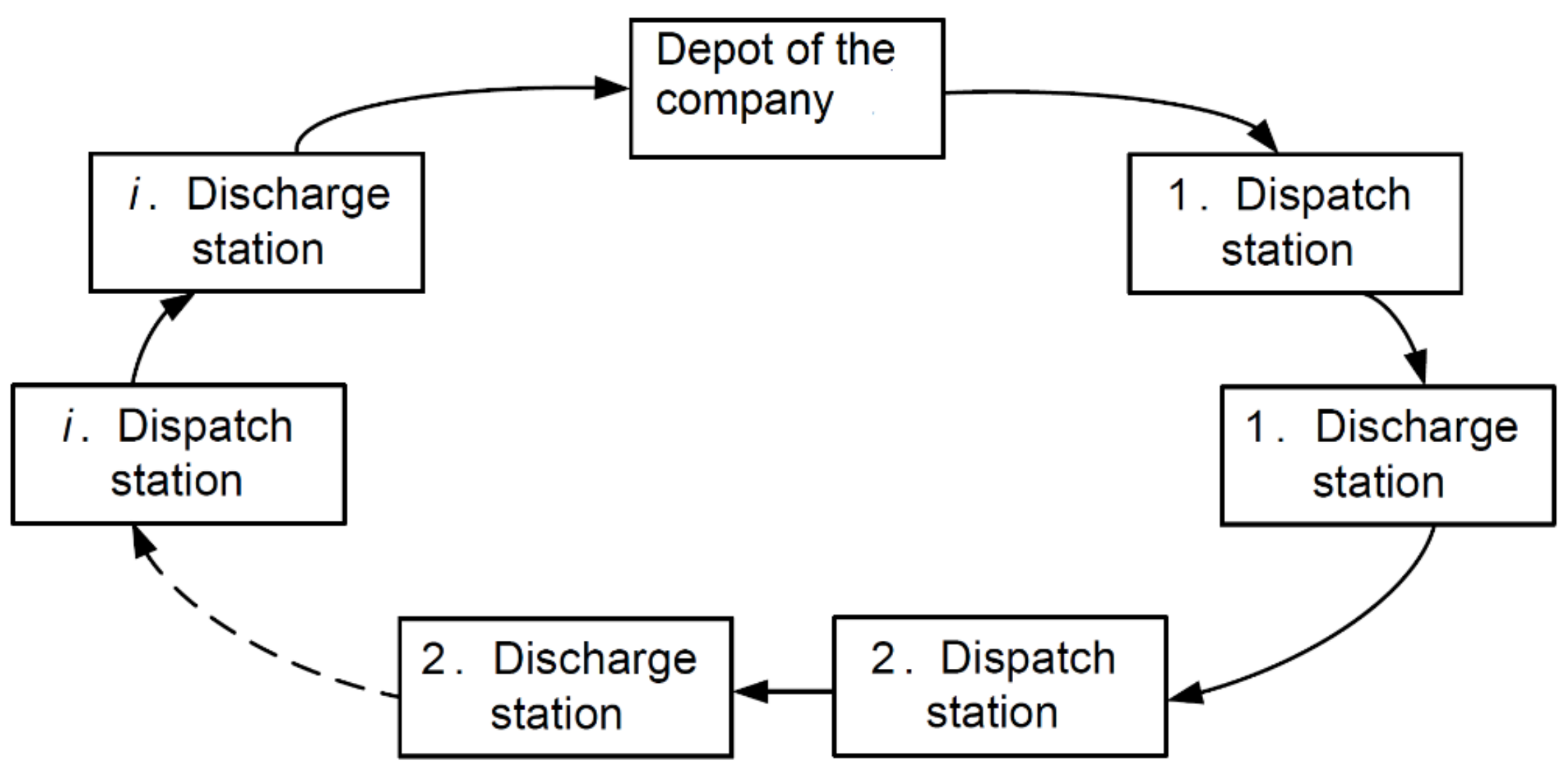
Transport loops generally start at the company depot and go on to the first product dispatch point. They then proceed to the first discharge station and go to the following dispatch and discharge points (
Figure 1).
After leaving the last discharge station, the vehicle finishes its route at the depot. The number of dispatch points/discharge stations can be arbitrarily chosen on a transport route; furthermore, any dispatch point can also be a discharge station [
30,
48].
The task was to specify a transport route for the driver from the starting point, determined by the coordinates x, y, to a given destination. It involved knowing the starting fuel level and the fuel consumption of the vehicle. Among the stations specified by the company, we determined the one fueling station where he or she should refill the tank of the vehicle. The aims were to achieve the most cost-effective transport route and to determine the necessary fuel quantity for the refill in order to safely complete the specific transport.
Due to their significant fuel consumption, most transport companies can buy fuel at a discounted price at a contracted fuel distributor. When choosing their fuel supplier, transport companies prefer companies with a Europe-wide fuel station network.
With the aid of the methods presented above, we were able to determine the shortest route between any two chosen points (e.g., between a depot and a fueling station, or between the dispatch point and the discharge station). Then, from all the qualified fueling stations, we selected those potential stations from the specified area, thus significantly reducing the number of variables within the final model.
When the transport vehicle was dispatched, we were aware of the starting point—i.e., the depot or the discharge station no.
i (
Li)—as well as the product dispatch point (
Fi+1) and the discharge station of the destination (
Li+1) (
Figure 2).
Therefore, we determined whether the vehicle was able to complete the entire transportation task with the known starting fuel level or if it had to refuel between the product dispatch points and the discharge stations. If refueling was necessary, we had to determine the ideal fueling station and the refill quantity.
During these calculations, transport routes were divided into sections, with each section representing the route between a dispatch point and a discharge station. This step was necessary since the values of the individual cost components differed during the completion of the individual sections, depending on the payload, the various road conditions, and other aspects.
The cost resulting from completing the road sections can be calculated according to the following formula:
where:
represents the route length (in kilometers) for the
-th transport of the
-th section;
is the specific cost for the -transport of the -th section ;
notes the section identifier.
Fuel consumption depends on the consumption of the unloaded vehicle, the weight of the payload, and the topographical conditions.
where:
represents the fuel unit price
; and
is the specific fuel consumption for an empty vehicle
;
is the correction factor for fuel consumption depending on topographical conditions, varying between the values 0, normal (flatland), 0.3, medium (hill areas), and 0.6, difficult (uphill);
is the correction factor for different loading conditions, since every additional ton of payload results in an extra fuel consumption of 0.5 L ; and is the vehicle payload .
The determination of the correction factors was based on previous research and on our development activity carried out for a transport company, which also included the evaluation of their transport activities.
The fuel level of the vehicle is known at the starting point (
), and the vehicle’s fuel consumption can be continuously calculated between dispatch stations and discharge stations (
Figure 2).
For the mathematical determination of the ideal refueling station, it is necessary for the vehicle to have a fuel safety reserve. This fuel reserve covers the extra consumption between points and in case of detours or if the driver loses his way, so that the road section is safely traversed. This safety fuel level can be determined as a specific quantity or as a percentage of the transport distance. The minimally required fuel amount for the vehicle to return to the company depot can be defined similarly. Let us designate this quantity as . This fuel amount ensures that the vehicle can refuel at the depot or at the station nearest to it with the necessary amount of fuel in order to start its next transport route ().
Given the above determinations and the requirements related to the safety amount level (
), we were able to calculate the distance between the current location and the first fueling station (
) (
Figure 2).
This radius arch () defines the coordinates of the potential fueling stations, from which the ideal station should be selected. The value of can be freely defined, and it refers to the distance at which a suitable fueling station has to be selected before running out of fuel.
4.2. Determination of the Optimal Fueling Station and the Amount of Fuel to Be Supplied
The optimal fueling stations were chosen from previously selected ideal fueling stations. Although this pre-selection was not necessary for the model, it considerably simplified the solution for the practical problem and also significantly reduced the size of our model. In the following section, we define the model in a more general manner than is needed for solving the practical problem presented above in order to ensure the possibility of the model’s further development. We supply the previously determined data and the variables, adapting them to the mathematical model, and thus we also specify the necessary notations.
4.2.1. The Known Data
A specific transport plan specifies those locations (dispatch points and discharge stations) considered from the perspective of freight logistics. The order of these locations is predetermined, and we used this order for identifying the dispatch points and the discharge stations. N notes the number of dispatch points and discharge stations, including the point of departure and the final destination (these two can coincide for transport loops, but we will designate them with two different indexes in this case). Each dispatch point and discharge station is noted with a natural number between 1 and N. Hereinafter, we will not differentiate between dispatch points and discharge stations; instead, we designate them generally as hubs. The original practical problem does not include dispatch points and discharge stations as such. In our model, we present these two concepts in a more general manner. In our approach, hubs can be used both for dispatching goods and for discharging goods. In the following, a hub is a dispatch point if the weight of the goods transported on the vehicle is less before arriving to the hub than after leaving it. In the opposite case, the hub will be a discharge station. The starting point is a dispatch point if the vehicle does not leave it empty, and the destination is a discharge station if the vehicle does not arrive there in an empty state.
4.2.2. Definitions
Road section. Hereinafter, a road section is the set of roads between a dispatch point or a discharge station and the next dispatch point or the discharge stations according to the transport plan. In practice, several routes can exist between two hubs, and we define these at the fueling stations. Road sections are noted using i indexes.
Consequently, we were able to easily identify the transport and, within it, the effectively existing road section with the hubs of the transport route. We also determined the identifiers of the road sections assigned to the hubs (road sections will be noted with the k index), since this identification was more appropriate for the computerized solution.
Set of fueling stations and potential road section. Let stand for the set of fueling stations between the i-th departure station and the -th destination point. In this case, designates the number of fueling stations on the i-th road section (the index of the road section corresponds to the index of its starting point). A specific route of the road section assigned to the fuel stations is called a potential road section, and it is designated with the indexes i, k. A possible road section must include only one fueling station. If there is more than one fueling station, then the model can be modified to a form in which there is, at most, one fueling station on each road section (see also the statement in Remark 4).
Notation of fueling stations: stands for fueling station k (i.e., the fueling station belonging to the k-th potential road section) on road section i.
The maximum number of fueling stations on a road section. () notes the maximum number of the petrol stations on a road section. For the i-th road section on which the number of fueling stations is less than H, we defined fictive potential road sections . The length of the potential road section should be high enough to ensure that it will not be chosen during the optimization process. This also ensures that it is indifferent within the model if we apply the analysis to the potential road section or H on a road section (the two values are interchangeable). The 0-th route (the route with the 0 index) is the road section without a fuel refill station. The vehicle does not stop on this potential road section, and there is no refueling in this case.
Topographical conditions. Two topography-related variables were assigned to the potential road sections in this model. One variable was the topographical factor assigned to the road section from the point of departure of the potential road section to the fueling station, and the other variable was the topographical factor assigned to the road section from the fueling station to the end point of the potential road section.
notes the topographical factor of the potential road section up to the k-th fueling station in the relation .
notes the topographical factor of the potential road section from the k-th fueling station in the relation .
Loading factor. notes the correction factor for different loading conditions (See also (2)).
Unit price matrix. notes the fuel unit price at the fueling station (). .
Distance matrices. Similar to topographical factors, the data related to distances were divided in two categories: data related to the length of the road section from the point of departure to the fueling station and data about the length of the road section from the fueling station to the destination point.
notes the length of the road section from the i-th departure station (with destination station ) to the k-th fueling station ().
notes the length of the road section from the i-th departure station (with destination station ) between the k-th fueling station and the destination ().
A definition of the i-th road section length was also necessary: ().
The vector of the quantities to be transported. notes the amount of load in the relation . It is 0 in case of empty runs. Thus, both loaded transports and empty runs received uniform treatment ().
Specific fuel consumption. notes specific fuel consumption (); see also at (2).
Fuel tank capacity. notes the maximum capacity of the fuel tank.
4.2.3. Remarks
Remark 1. Due to computational reasons, the indexes start from 0 and end at H in the case of the matrices L, M, S, and P.
Remark 2. For practical reasons, in the case of 0-th road, the total length assigned to l is m = 0 (, ).
Remark 3. When it is possible to refill the tank on the highway as well, which is the 0-th road, then this road must be defined again, with the indexes l and m assigned to the fueling station. In this case, two potential road sections corresponded to the highway road section, and both had the same characteristics (length and topographical conditions). Thus, choosing the road section with the 0 index means continuing the transport without refueling, while choosing the road section with an index different from 0 means refueling on the highway section. If there is more than one fueling station on the highway, the procedure described in Statement 1 below should be followed.
Remark 4. There are two possible ways to proceed from one hub to the next:
- (a)
Based on free choice, i.e., the freedom to choose among the potential road sections;
- (b)
Through mandatory proceeding, i.e., if we arrive from k-th potential road section, then the next hub must also be approached through the k-th road section. The significance of this is explained in more detail below.
4.3. The Mutual Assignment of Fuel Stations and Potential Road Sections
In practice, several fueling stations can exist on a potential road section between a dispatch point and a discharge station. For reasons associated with manageability, we assumed within the mathematical model supplied below that only one fueling station was present on every potential road section (which also made it easier to solve the practical problem). The model related to the practical problem can be converted into a model meeting the condition of one fueling station, at most, on a potential road section. The following two statements further illustrate this idea.
Statement 1. The original problem can always be converted into a task in which there is one fueling station, at most, between two hubs.
Any potential road section can be divided into many potential road sections if there are more fueling stations on the same potential road section. In the original problem, each hub is designated as freely chosen (
Figure 3).
Two cases can be distinguished from this statement.
Case 1: In the first case, let us consider those potential road sections with more than one fueling station for which it is true that any of their fueling stations can be reached from one of the fueling stations of the previous potential route sections if the vehicle’s tank was filled fully at any of these fueling stations. In practice, this means that any fueling station of the potential road section can be reached without having to resort to another fueling station on section
Let us select such a potential road section and divide it into as many road sections as there are fueling stations, similar to section (3) of the previous remark (
Figure 4). Let us implement this step for all potential road sections of this kind. Thus, we have substituted the previous potential road sections fulfilling the condition with several potential road sections corresponding to the requirements of the model.
Example 1. There are two fueling stations on a potential road section according to the conditions of Case 1.
Case 2: If Case 1 cannot be implemented, this means that the potential road section has a fueling station that is unreachable directly with a full tank from any of the fueling stations of the previous potential road section. In other words, there is a fueling station on the potential road section that can only be reached if refueling has already occurred at this potential road section. In this case, let us insert a fictional hub for the
i-th road section between the original road section in such a way that it will lie between two fueling stations of the potential road section, and that the condition of traversing the individual potential road sections is fulfilled (
Figure 5). Now, the fictional point must be designated and the potential road section must be divided for all potential road sections of the relation
. This can be any point in the relation, except a point belonging to the fueling station of the potential road section (for computational reasons). The divided road sections are indexed in such a way that the k index of the road section arriving at the fictional hub corresponds to the index of the potential road section starting from the fictional hub of the divided road section. Next, this assigned hub has to be designated as a hub for which it is mandatory to pass through (
Figure 5). If the condition remained unfulfilled, we implemented the steps described in Case 2 until the expected condition of the model was fulfilled. In other words, we implemented the steps until arriving at a road section without a fueling station that could not be traversed (nevertheless, the problem was still solvable).
The hub through which it is mandatory to pass through must be introduced because, although we divided the original road section into two potential road sections, the continuation of our route could not be freely chosen—as opposed to the previous cases—since we could only reach the second fueling station on the condition of refueling at the first fueling station. At the same time, the insertion of this hub ensured that there was one hub, at most, on a potential road section.
Example 2. Two fueling stations are on a potential road section according to the conditions of Case 2.
The starting situation is formally similar to the situation represented in
Figure 3. However, in
Figure 3, the
k and
k + 1 fueling station can be reached with a full tank from one of the fueling stations of the previous potential road section, while in the present starting situation, the
k + 1 fueling station cannot be reached from any of the fueling stations found in the previous section.
4.4. The Unknown Factors of the Model
The following matrix contains the first group of the variables. The elements of it define the amount of refilled fuel at each road section.
will note the amount of refilled fuel at the
k-th fueling station between the
i-th departure station and the
-th destination station. If
, then there is no refueling on the given section, so that the amount is a fictive quantity
. This does not cause any problems, since this 0 variable will not appear in the costs and in the fuel consumption.
We can deal with the following situation with the aid of the signum function: if we have refueled with more than 0 L of petrol, then there is refueling, represented by the value 1. If we have refueled with the quantity 0, then the value of the refueling is 0. In other words, there was no refueling. Accordingly:
i.e., one of the possible routes should be selected.
We can determine the length of the entire route using the previous formula. This is not included in the model, but it is both important and necessary for planning aspects of the transport, such as its duration, rest periods, and the number of drivers. Thus:
means the length of the road section between
i and
, if refueling at the
k-th fueling station. Based on these data and taking into account the detours necessary for refueling, the total length of the route completed by the vehicle is:
Let
denote the amount of fuel in the vehicle at hub
i.
In this case, the amount of fuel at the hub following the refueling can be defined as:
meaning that the amount of available fuel at the previous hub is reduced with the consumption depending on the load and weight, but it is increased with the amount refueled on the road section.
A further requirement is that the amount of fuel cannot drop under a minimum safety level. This minimal amount of fuel has to be available for the vehicle at the fueling station. At the current refueling station, the amount of available fuel is equal to the amount of fuel available at the last hub, reduced by the amount of fuel consumed on the route leading up to the fueling station:
The amount of refilled fuel (
) cannot exceed the capacity of the tank. This is determined by the difference between the dimensions of the fuel tank and the amount of fuel left in the tank:
Let O denote the set of the indexes of the mandatory hubs. In this case, we have to go through the same potential road section with the index k on which we arrived.
In this case, the following condition applies to the mandatory hubs:
When arriving at the destination (
), the vehicle should have a certain amount of fuel available (
) in order to be adequately prepared for the next route:
Let
denote the cost of the amount refueled for the relation
(if there was no refueling, then 0). Furthermore:
The cost of refueling at the given fueling station is:
Remark
We will use condition (9) in the following form:
In (16), the index k starts from 1, and the 0 index is emphasized. This is because there is no refueling at fueling station 0. Thus, can take on any value, and it will not influence the amount of fuel in the tank. In the objective function, it is not included among the costs because of the 0 price. Incidentally, as we described above, if there is no refueling at a given road section, then the value x of the corresponding road section 0 will be greater than 0. This is a “fictional” tanking, when fuel is not actually introduced in the fuel tank.
4.5. The Objective Function Applied during Optimization
The objective function signifies the fuel cost of the starting tank (which is a fixed cost), reducing the amount of fuel refilled on the route with the cost of the remaining fuel (variable cost):
The above formula means that the cost of the remaining fuel has to be reduced with the unit price at which we bought it, i.e., the cost at the last fueling station.
Thus, the problem can be stated as a mathematical programming task.
Remarks on the objective function (17):
During the computing solution, for practical reasons, we can start the k index from 0. This means that we can also include the routes with no fueling stations without influencing the result.
2.
can be omitted during optimization, since this is a constant and thus does not influence the optimum. Therefore, it can be signified as:
4.6. Simplifying the Model Used for Determining the Location of the Optimal Fueling Station and the Amount of Fuel to Be Refilled
During modeling, it was necessary to use the sign function, which can cause problems in the solution process. In order to eliminate these problems, let us introduce the
Convert the condition:
according to the following:
Then, the condition of the mandatory hubs can be easily converted. In the modified model, the condition:
corresponds to condition (13). Thus, condition (10) will be modified as follows:
The problem is caused by the formula of condition (25):
signifying the multiplication of two variables. In fact, if
, then
, and if
, then
. It follows that
because of Equation (23).
Consequently, condition (25) will be the following:
Thus, the condition is converted into a linear condition.
4.7. The Final Model for Determining the Location of the Optimal Fueling Station and the Amount of Fuel to Be Refilled
The set of conditions of the final model is as follows (with constants arranged to the right side):
Based on the above cost components, the following objective function can be supplied for the model:
Statement 2. As demonstrated, even if only one refueling has taken place, the vehicle will reach the depot with the specified minimum amount of fuel ().
Demonstration. The amount of fuel with which the vehicle arrives cannot be less because of condition (37). Let us suppose that this solution is optimal, but the vehicle arrives with more than the minimum amount of fuel. Now take the difference between the current amount and the safety amount (), and subtract it from the amount of the last refueling. This leads to a lower cost, which contradicts with the statement that the original solution was optimal.
Because of the statement, the remaining amount
was not necessary for the calculations, and thus was omitted. It was also possible to prevent refueling under a minimal amount at a fueling station. For this, we determined that the following condition had to be added to the model:
5. The Optimization Task and Its Solution Method—Case Study
After specifying the model, we sought to demonstrate that the task related to the model is solvable and that applications are available that can effectively solve the problem. Our ultimate goal was to develop a program module related to the dispatching system of companies. The final module was built on a data base [
64,
65,
66,
67,
68], and solves the practical problems in a similar, user-friendly way.
Hereinafter, we demonstrate the solvability of the task and the applicability of the model through an example task we solved using the MS Excel Solver. We chose the non-linear AVG method (gradient method) of Solver [
69,
70,
71,
72,
73] as the solution method. It should be noted that in addition to the solution presented, we also tested it with MATLAB and obtained the same result.
5.1. The Example Task and Its Data
In this section, we apply the mathematical model and detail the solution of the problem for an example task.
Let us consider a transport loop with four hubs. There are two fueling stations between hubs 1 and 2, three fueling station between hubs 2 and 3, and only one fueling station between hubs 4 and 1. There are no fueling stations between hubs 3 and 4. Between all neighboring hubs, there is a potential road section with no fueling station, established according to Remark 3 following the Definitions (
Figure 6). Additionally, according to this remark, there is only one fueling station on every potential road section. The destination station has its own fueling station, and the motor vehicle can thus refuel here after arrival.
Subsequently, we define the values of the individual data (the data are fictional and may, in certain cases, differ from real-life technical parameters).
.
.
Load factor: .
Safety fuel level: ].
Fuel consumption in the case of an empty vehicle:
]
“Max” is a sufficiently high value in this case. Generally, a sufficiently high value has to be chosen in order to avoid the situation in which the fictional fueling station is included among the chosen fueling stations during optimization (for example, we have set the Max value at 100,000 Euros in Excel).
Topographical conditions:
In our example task, we assumed that the possibility for refueling exists at the final destination. Thus, it is sufficient if a fuel amount corresponding to the safety level remains in the tank of the motor vehicle. In other words: .
5.2. The Solution of the Example Task Using MS Excel Solver
Due to its size, we can only present the computational model corresponding to the mathematical model of the example task in a figure. In column A of the table, we have indicated the relation of the individual conditions and the conditions of the model to which the individual rows belong. Formally and structurally, the computational model will look according to the
Appendix A.
We can include the limiting conditions in six groups according to the relations in column A1 of
Appendix A, and it is sufficient to set only one limiting condition for these groups in Solver. Condition (7) ensures the bivalence of the y variables. The other variables are not negative according to the model, which is set through checking the option “Make unconstrained variables non-negative”. We chose the non-linear AVG as the solution method.
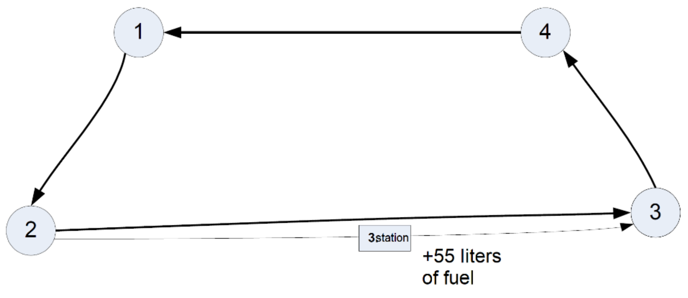
5.3. The Significance of the Result Obtained Through Optimization
Solver found an optimal (or close to optimal) solution for the task after a short run. According to the obtained result, we will refuel once, between hubs 2 and 3, with 55 L of fuel, at fueling station 3 (
Figure 7).
Without conducting a more detailed analysis, or a sensitivity analysis, we present some results on the basis of the above example, obtained through modifying the input values and the goal. The results of Solver show that if we haphazardly choose the fueling stations and the route of the transport loops or leave this choice entirely to the driver, then we will record major losses.
If we optimize on the basis of the shortest route (keeping the conditions for refueling unchanged), then the route would be reduced from 1310 km to 1250 km (to 95.4%). At the same time, the determining costs (i.e., the “reduced” cost from the objective function) will rise to 34% (from 55.44 to 74.31 Euros). If the driver chooses the shortest route, then he might reach his destination faster, but with the potential result of a significant increase in costs.
In terms of calculating the total cost, a 10% change in the fuel price in our example task would amount to a change of almost 5% compared to the total cost. In this case, it is also important to take into account that the transport is of a very special kind. If a more significant increase in fuel prices occurs, the cost of refueling will appear as a greater percentage among the transportation costs (in our example, the increase amounts to approximately 5%). Consequently, the right choice when selecting fueling stations is especially important in these cases.
If we look for the most expensive solution under the above conditions (for the depot of the company, refueling only on the highway, with the maximum amount), then our total cost would be 62.33 Euros (an increase of 12%, with only two refueling possibilities), which is already a sizeable difference. This also indicates that the conscious selection of fueling stations represents an important issue in the reduction of logistical costs.
6. Conclusions
We developed a new precise and reliable optimization method for the minimization of road freight transport costs. In doing so, we aimed to reduce fuel costs by determining the optimal fueling station and to calculate the optimal quantity of fuel to refill.
This decision-supporting mathematical method is an efficient solution for the optimal fuel supply of transport activity. The application of the new method supports drivers’ decision-making concerning the optimal fuel station at which to refuel and how much fuel is necessary for refueling in order to reduce the fuel consumption and fuel costs. However, in practice, transport companies have not used mathematical methods and have instead relied on the ad-hoc decisions of their drivers. In doing so, they have incurred cost- and time-related losses.
As discussed in this paper, our optimization method involves two key phases:
In the first phase, the optimal, most cost-effective fuel station is determined based on the zone of the potential fuel stations. The specific fuel prices differ per fuel station, and the stations are located at different distances from the main transport way. Our method can determine the optimal fuel station, i.e., the most cost-effective fuel station based on the specific fuel prices and additional transport distances. The method enables drivers to determine whether refueling at a farther but cheaper fuel station or at a nearer but more expensive fuel station is more economical.
In the second phase, the optimal volume of the fuel is calculated. In other words, this phase focuses on the exact volume of fuel needed, including an adequate amount to cover stochastic incidents (e.g., additional consumption due to road closures). The optimal amount of fuel to be refilled refers to the volume required to achieve the given transport task. The determination of the optimal fuel volume is important. Specifically, if the amount of refilled fuel is less than the optimal volume, drivers have to find another fuel station and refuel their vehicles, thus resulting in additional costs and time losses. Moreover, if the amount of the refilled fuel is higher than the optimal volume—especially near to end of the transport loop—then it is also a loss, because drivers can refill with the cheapest fuel at the depot of the transport companies.
The main contribution of our optimization method is its support to the drivers’ optimal decision-making. It enables them to determine the optimal fuel station and the amount of fuel for refueling in order to reduce the total fuel cost. Therefore, the application of the new optimization method compared to the recently applied ad-hoc decision-making of the drivers results in significant fuel cost savings.
A case study confirmed the efficiency of our optimization method. As the case study showed, the optimization of the fuel supply results in a reduction in fuel consumption and cost as well as less environmental damage.
Previous studies highlighted available methods for route optimization and the optimization of transport trips and networks. However, these studies did not focus on an optimization method for the minimization of fuel costs based on the optimization of the fuel supply. Therefore, as mentioned, we did not have a comparable method available to analyze. Because of the uniqueness of our method, we could only compare it to the drivers’ ad-hoc individual decision-making. Based on this comparison, we determined that the application of the method results in the reduction of fuel consumption and, correspondingly, significant cost savings for transport companies.
Our optimization method is applicable to sparsely populated areas where the number of fuel stations available to drivers is small. One of our future research plans is to develop a software program for planning the optimal fuel supply—based on the new optimization method—in order to minimize the fuel costs. Small- and medium-sized transport companies in particular could widely apply this software in practice.


