A Procedure for Automating Energy Analyses in the BIM Context Exploiting Artificial Neural Networks and Transfer Learning Technique

Abstract

One of the main benefits of Building Information Modelling is the capability of improving the decision-making process thanks performing what-if tests on digital twins of the building to be realized. Pairing BIM models to Building Energy Models allows designers to determine in advance the energy consumption of the building, improving sustainability of the construction. The challenge is to consider as many elements involved in the energy balance as possible and shuffling their parameters within a certain range. In this work, the automatic creation of a relevant set of design options to be analyzed for searching the optimum has been carried out. Firstly, the usual workflow that would be applied manually has been automatically followed by running scripts and codes, depending just on the initial setup given by the user. Although the procedure is very resource consuming, the main advancement relies in the reduction of the manual intervention and the possibility of creating large datasets of design options, avoiding gross errors. Secondly, Artificial Neural Networks and Transfer Learning techniques are applied to speed up the process of dataset creation. With such approach, the same dataset has been created, with about 30% of initial data and without significant loss of accuracy.

1. Introduction

Building Information Modeling (BIM) has been used to transform the Architectural Engineering Construction (AEC) industry or rather the way buildings are designed, constructed, maintained operational and even dismissed or renewed. In the whole life cycle of a building, BIM technology is also being used to provide accurate, timely and relevant information, dramatically improving the effectiveness of asset management [1]. By shifting efforts in the early stages of a project, BIM enables designers to model structures before they are built with great impact on decision-making of all involved stakeholders. In fact, by exploiting the BIM approach and related technologies, architects, engineers, and building owners can explore multiple options when planning for or manage facilities, infrastructure, and environment. By creating a virtual model and applying different techniques, materials, and designs, prior to the beginning of construction, reliable predictions can be made about cost, functionality, stability and more [2].

Today, most stakeholders understand the implications and possibilities enabled by using BIM as a tool to facilitate information flow and support better decision-making throughout the building lifecycle. Among all the aspects, sustainability has raised the profile of building lifecycle management [3]. The importance of long-term sustainable construction in our current social climate is indisputable. BIM technology is a tool that is being used to help make the AEC industry more economically and environmentally sustainable [4].

In this context, digital twins of buildings are tied to Building Energy Models (BEM) allowing designers to perform what-if tests to determine the energy consumption of the building, helping reduce waste and overall building costs. When BEM tool is integrated within the BIM application and workflow, energy analyses can occur as early as the concept stage, allowing for more informed design decisions [5]. Energy modeling tools use a range of parameters to estimate the energy performance of a building. Some of this information, e.g., building envelope, zones, rooms, structure, equipment, control scenarios, can often come directly from the BIM system. However, for comprehensive energy modeling, a more detailed level of information on energy characteristics is needed [6]. BIM model is made up of various categories of ‘objects’, which include each unit of equipment in the building. Objects can include different levels of detail, often provided by the equipment manufacturer, which needs to be in a format the specific BIM system can understand [7]. For effective energy modeling, the designer needs to include the right amount of information about each piece of equipment or component, including at the very least: power consumption, heating and cooling capacity (for HVAC equipment), thermal characteristics and behavior (for passive systems).

The challenge is to consider as many elements involved in the energy balance as possible and shuffling their parameters in a plausible and meaningful range [8]. The permutation of all considered design components and energy properties realize a set of combinations among which the optimal solution must be searched. This optimization problem can then be solved under different perspectives (e.g., minimum cost, best performance and many others) [9,10,11]. Further complicating things is the fact that BIM design typically uses multiple tools, each with a different focus, and separate BEM tools for energy modeling. This requires data to be transferred between the BIM and BEM models, which is more difficult and time-consuming when the tools are not integrated [12,13] or used through a platform that manages them jointly [14]. Standards exist that enable the extraction and sharing of data between BIM and BEM tools, including the Industry Foundation Classes (IFC) and Green Building XML (gbXML). However, these require a middleware conversion utility, and there is room for potential errors along the way or missing data during the conversion process [15,16,17,18,19].

In terms of environmental sustainability, many factors are involved when computing the energetic balance of a building, also interacting one to each other differently. Several studies analyze this aspect, exploiting BIM technology and its capability of virtualizing the design and construction process, therefore being able to perform preliminary analysis in a more exhaustive way. In [20], BIM is used to perform a parametric analysis aimed at designing the building performance parameters based on climate conditions towards energy efficiency. They studied various design standards (exterior walls material, roofs material and a set of window-to-wall ratios) in combination with building location. The researcher found through results around $15\%$ improvement in the energy consumption due to change design options such as window-to-wall ratio, disregarding the location. Piselli et al. [21] analyzed the impact of energy plant replacement for the retrofit of existing buildings. Ground source heat pump system and existing gas boiler were compared and results showed up to $73\%$ heating energy need reduction and $69\%$ CO₂ emission savings while maintaining the same operation and comfort conditions for the occupants. Taha et al. [22] performed daylight and photovoltaic panel performance analyses on a modelled two-floor educational facility. They quantified also the energy saving led by design alternatives in terms of kWh/year, experimenting the use of BIM technology for preliminary design assessments. In [23], De Gaetani et al. investigated the interdependency of main building components in terms of both costs and energy consumption. They found that depending on the expected life cycle of the building, the priority of investments on more performing technologies should be accurately analyzed, being that not obvious. Mohelníková et al. [24] analyzed several options for complex retrofits focused on building envelopes and their window/shading systems together with the installation of efficient technical systems for HVAC systems. Their analyses on heating energy demands in existing old buildings showed the importance of renovations for their energy efficiency. On the other hands, the thermal and daylight evaluation results showed that renovation improvements could be sometimes counter-productive from the indoor comfort point of view.

The aforementioned researches are based on the generation of several BIM models by differently combining factors influencing the energy analysis, carried out subsequently the BIM modeling process. The objective was not finding the optimum in absolute terms but identifying factors more affecting the energy balance or comparing different design options. The bottle-neck of such comparisons were the limited amount of investigable alternatives, due to operational and practical reasons. Among all the possible solutions there are the automation of the whole process of modeling and analysis of the building or the estimate of intermediate options so to densify the set of design alternatives. In this context, approaches using BIM include work by [25] who created a generative design system on top of Autodesk Revit [26] that manipulates window sizes and invokes the Autodesk Green Building Studio API [27] to determine the resulting energy-analysis metric. In a subsequent work [28], the authors used Autodesk Dynamo [29], a visual-programming tool, to solve a similar problem, namely that of discrete window-size optimization for reducing daylight usage and energy consumption. In [30], a framework for optimization BPOpt (BIM Performance Optimization) based on Dynamo was created, which breaks the generative design into fives phases: decision variables (input), initial random population (initial setup), fitness functions (evaluation), generation loop (decision making), and writing to CSV File (output). Depending on the problem the user plans to optimize, they could alter the input parameters and develop the appropriate fitness functions, thereby making the problem seemingly independent of the type of generative design.

However, recent advances in Information Technology have led to a new breed of computer-based tools. Artificial Neural Networks (ANNs) are one of the best and most widely utilized tools in the development of prediction models in different fields and BIM exploitation for energy analysis is one of these. Alshibani and Alshamrani [31] described the development, testing, and validation of a conceptual system to assist architects in selecting the optimum alternative design that minimizes the cost of energy consumption of residential buildings in Saudi Arabia. The proposed system incorporated BIM and ANN-based models to predict energy cost. Different ANN models with different characteristics were tested and built using real data on energy consumption collected from six cities across the eastern province of the country. In [32], Ma et al. evaluated indoor personal thermal comfort for a comfortable and green thermal environment. They proposed a BIM-ANN based system for this purpose. The system included an ANN predictive model considering three environment parameters (air temperature, air humidity, and wind speed around the person), three human state parameters (human metabolism rate, clothing thermal resistance, and the body position) and four body parameters (gender, age, height, and weight) as inputs. In [33], the research focused on developing robust ANNs for use as surrogate models for simulation by using data generated from the Simulation-Based Multi-Objective Optimization (SBMO) model developed in a previous research [34].

The outcome of this study showed that the proposed ANN models could efficiently predict the total energy consumption, life-cycle cost and life-cycle assessment for the whole building renovation scenarios considering the building envelope, HVAC, and lighting systems.

In this work, a framework for automatic creation of large datasets where searching the optimal combination of a set of given parameters of a BIM model is proposed, facing also the problem of how to speed up the whole procedure. Such approach has been implemented in two main steps. Firstly exploiting the possibility of automating the model generation and analysis given by interfacing the involved software packages with scripts and codes that replicate the human intervention avoiding gross errors and allows for managing the complete procedure from an initial setup. Secondly, Artificial Neural Networks and Transfer Learning technique has been applied, aiming at speeding up the dataset creation and increasing the parameters range resolution on the basis of a subset of available design alternatives.

2. Methodology

In this work, the automatic creation of a relevant set of design options to be analyzed for searching the optimum was carried out in two main steps. In the first step, the usual workflow that would be applied manually was followed by running scripts and codes that perform each stage (i.e., parameters setup, model creation, energy analysis, results evaluation) sequentially and depending just on the initial setup given by the user. This allowed a quick creation of design alternatives by greatly reducing the manual intervention and consequently the possibility of gross errors and loss of time. At the end of this first step a great amount of data could already be obtained but the process was time-consuming and intermediate solutions should be obtained by repeating the scripts with different setups. This aspect could be faced by exploiting the results of this first step as input for predicting (instead of computing) the desired intermediate solutions. In the second step of the proposed approach, ANNs were applied to increase the resolution of parameters range and Transfer Learning technique was applied aiming at allowing the possibility of evaluating options that were not considered in the initial setup. The following subsections focus on the description of these two main steps that are the framework of the proposed approach.

2.1. Automatic Design Options Creation

With the aim to build a framework that automates design options creation for energy analysis, a relevant dataset had to be built as a first step. At the first stage, for energy analysis, the following parameters of a building were accounted for: window-to-wall ratio (WWR), shape of the building, rotation in plan, thermal characteristics of elements such as floor, walls and roof. Each parameter had a certain range of variations, thus for a complete analysis, each combination was considered. The general workflow of this step is presented in Figure 1:

After having determined the range of parameters of interest at the first stage, each combination of these parameters was applied to an Autodesk Revit model one by one. This was done using Revit API and Python programming language: they together made it possible to interact with the authoring software through code. As combinations were applied, current state of the Revit model is saved in gbXML file format, where each gbXML file described the Revit model with a specific applied set of parameters from an energetic point of view. Therefore, the output of the second stage was a collection of gbXML files, with each file being a design option.

At the third stage, to conduct energy analyses of this collection of data, these gbXML files were uploaded to Autodesk Green Building Studio using Dynamo, which is a part of the out of the box Revit and is a visual programming tool. The Dynamo package used was “Energy Analysis for Dynamo” [35], which requires a list of gbXML files created earlier, and a Green Building Studio project ID, specified in the ProjectID node on Figure 2. The ID can be found using GetProjectsList node from the package, given that a Green Building Studio project has already been created. Other than that, for Revit to be able to recognize the user, one must have logged in in the Revit environment with valid Autodesk credentials.

After this Dynamo script was run, each file was uploaded to Green Building Studio, and the energy analyses started automatically using DOE-2 engine. This concluded the third stage of the workflow.

Upon completion of the analyses, additional design alternatives based on previous design options were created. The additional design alternatives accounted for different WWR ratios and they were accounted for by creating so-called “alternative runs” using browser automation technique (i.e., Selenium Python package). GBS offers a wide range of parameters to change in alternative runs; however in this case, advantage was taken only of assigning different WWR ratios, which added the last level complexity to the analysis. It is important to note, that windows added by GBS had a default R value of 0.5 $\frac{W}{m^{2}K}$. Analyses of added alternatives started automatically, and when completed, the results were downloaded from the website using built-in function of GBS that allowed us to download reports in Excel format. The results represented a set of Energy Use Intensity (EUI) values for each design alternative. EUI estimated how good or bad a model performed from energy consumption standpoint and was measured in $\frac{kWh}{m^{2}year}$. The obtained EUI values were the output for any given configuration considered and could be used as input to train an ANN that could then predict additional EUI values for not considered configurations.

2.2. Design Options Prediction through ANN

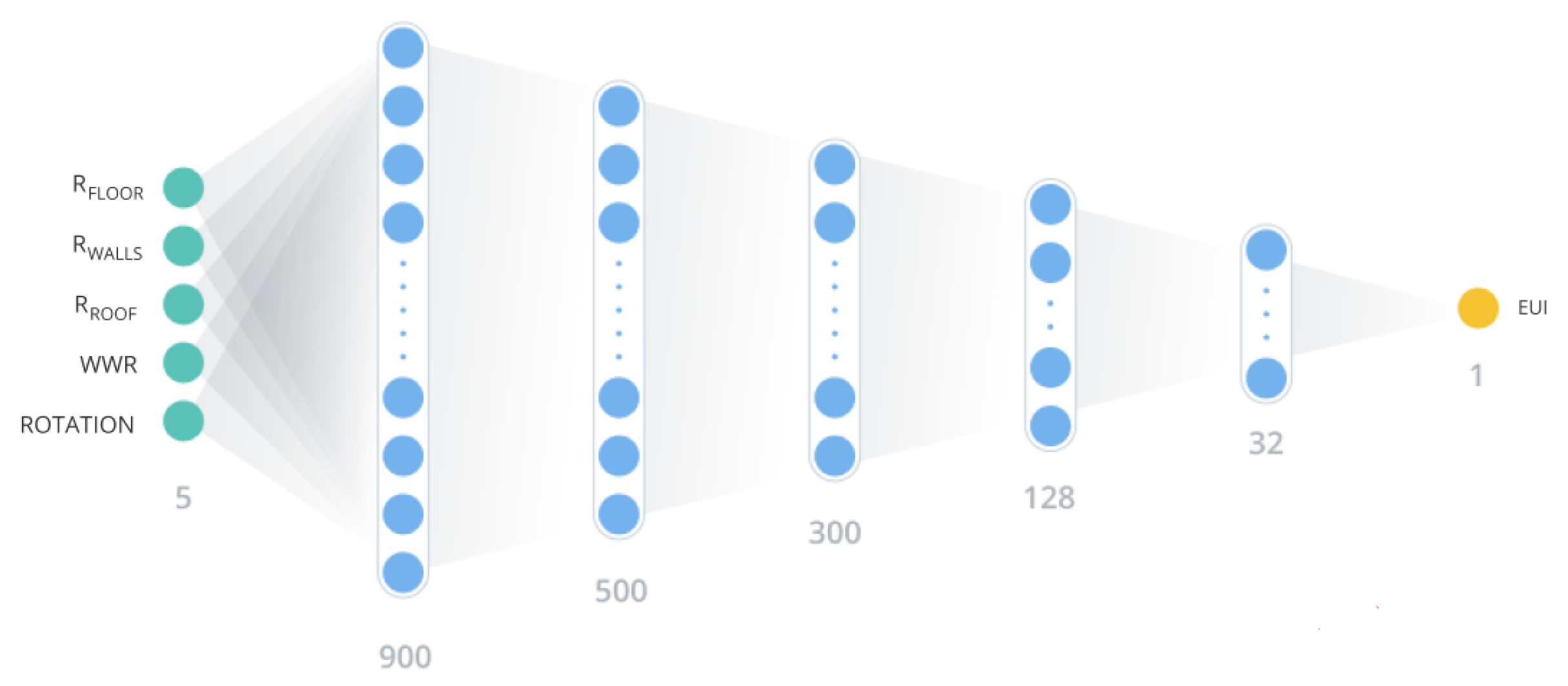
The body of an ANN can be thought of as a series of matrices with gradually decreasing size. To get a prediction of EUI, the input vector was multiplied by the first matrix, giving a vector that was in turn multiplied by the next matrix. This series of operations eventually led to a single number, which was the EUI prediction. Conceptually, just described ANN could be represented as in Figure 3:

Initially randomly generated values of the matrices got updated based on partial derivative of so-called loss function used to assess predictions after each iteration described above. This ensured that the prediction came closer to the ground truth value after each iteration. This process was called training of a neural network, where each neuron performed a weighted sum of the x values representing the input vector. By tuning the weights of the neuron w, each of of them was capable of fitting well only data with linear correlation, but if they were stuck atop each other, they formed a powerful system capable of fitting quite complex data, which was indeed this case.

Usually, out of a dataset, a big amount of available data was used for training, and small fractions—for validating, i.e., some data points were left out of training process intentionally to check how good or bad the predictions based on part of the data were. However, if an ANN trained for a similar task was available, then so-called transfer learning could be applied. Transfer learning is a technique allowing to use already trained neural network and retrain it for a new dataset. This is feasible because an already trained ANN ‘knows’ how each input influences the outcome, therefore it knows general patterns. Therefore, if a new dataset represents about the same distribution as the one for which the existing ANN is trained, then with minor shifts of weights it is possible to make the ANN fit the new data. The main benefits of using this technique is that it takes less time and data to train an ANN built on other ANNs. In fact, being able to apply transfer learning has been the key consideration behind this particular choice of ML technique. Based on this reasoning, workflow depicted on Figure 4 emerges:

According to the workflow, first, an ANN was trained on a set of data, and the ANN was reused to be a foundation of other ANN to take advantage of Transfer Learning and estimate time savings and predictions accuracy.

3. Case Study

This section is devoted to a practical implementation of the workflow previously described. The considered parameters around which design optioneering revolved were those reflected in

Table 1. Design parameters.

Parameter	Range of Values
$R_{Floor}$	0.5–1–2–3–4–5–6–7–8–9–10–12.5 $\frac{m^{2}K}{W}$
$R_{Walls}$	0.5–1–2–3–4–5–6–7–8–9–10–12.5 $\frac{m^{2}K}{W}$
$R_{Roof}$	0.5–1–2–3–4–5–6–7–8–9–10–12.5 $\frac{m^{2}K}{W}$
Rotation	0°–45°
Shape	Box–Prism (same Box wall area)–Prism (same Box volume)
WWR	0%–50%–95%

.

Regarding the shape parameter, three different geometries of the Revit model were analyzed: a box shape and two hexagonal prisms reflecting the wall surface and the volume of the box reference shape. We called them Box A, Prism B and Prism C, respectively. The reason for having two hexagonal models was the following: when evaluating an influence of a parameter on a certain outcome, it is a good practice to change the parameter not influencing other ones, but in case of different shape it is not possible (EUI refers to unitary floor surfaces), so all variations conjugated with a shape change are accounted for.

As seen in

Table 2. Characteristics of the three considered model geometries.

Model Type	Floor Area, m2	Volume, m3	External Wall Surface, m2
Box A	94	310	144
Prism B	94	337	144
Prism C	94	310	155

, all options had the same floor area to exclude influence of this factor.

From Table 1 it is seen that number of combinations was 12·12·12·3·2·3 = 31,104. This large number of combinations required automation of their creation, which was achieved using Revit Python Shell for Revit.

All Revit models were created using a build-in Revit HVAC system definition; namely, Residential 14 SEER. It was kept constant throughout the study.

3.1. Creation of the Initial Dataset

As first step, thermal resistances of the materials of which the elements were made of were subject to iterative change. Thermal resistance of an element is $R=\frac{C}{h}$, where C is the thermal conductivity of the material measured in $\frac{W}{mK}$ and h is the element thickness. Therefore, knowing thickness of an element, it was possible to set desirable thermal resistance, changing the thermal conductivity value, which was accessible in Revit through the Material Browser and could be found as attribute of the material the element was made of. Revit API was used to iteratively change the value of thermal conductivity of each individual material, going through each combination of thermal resistances. The value of thermal resistance that had to be set on each iteration was calculated, h being known, as well as the desired R. To find each relevant material’s thermal asset, which is a Revit object holding all thermal characteristics of materials, the script in Appendix A as Listing 1 was run in Revit Python Shell with a Revit model opened.

Upon completion, those objects could be used to assign thermal resistances and subsequently convert each Revit model state to a gbXML representation using Revit API. The code in Appendix A as Listing 2 did that.

After each cycle of the loop, a rotation of 45° was applied to the current model to take into account of orientation of the model.

At this point, 10368 gbXML models had been created. The last factor, WWR, was accounted for on Green Building Studio website after all gbXML files were loaded onto the GBS using Dynamo node (see Figure 2) where all paths came from parsing the directory containing just obtained gbXML files, as per Python code in Appendix A as Listing 3.

Launch of this node marked the start of uploading process, after which energy analyses of the design options started automatically using DOE-2 engine implemented in GBS. Green Building Studio was then used to assign different WWRs for walls in North, South, West and East directions. This was usually done by manually creating an alternative run with the desired WWR but considering the number of alternative runs to be done, decision was made to resort to browser automation technique. Thus, after having collected URLs of all main ran into a single txt file, Listing 4 in Appendix A was implemented to assign all WWRs.

After this, 31104 design alternatives were created and analyzed. In fact, at the end of this stage GBS dashboard contained six projects with 5184 runs each. A summary of how the dashboard looked like is presented in

Table 3. Summary of the GBS dashboard at the end of the automatic analyses.

Project Id	Shape / Orientation	No. of Runs
1	Box A/0°	5184
2	Prism B/0°	5184
3	Prism C/0°	5184
4	Box A/45°	5184
5	Prism B/45°	5184
6	Prism C/45°	5184

:

The results of the analyses can be downloaded for further analyses aiming at finding the optimal configuration or assessing which, among the considered parameters, influenced the final result more. This would be out of the scope of the presented work but with such amount of design alternatives to be compared, a preliminary assessment can be done by plotting them. This can be done by fixing three of the six considered parameters under investigation so to be able to plot the EUI values obtained as function of the remaining three parameters free to vary in their assigned range. An example is provided in Figure 5.

The cube in Figure 5 is identified by 1728 points where each point represents a single combination of thermal resistance of walls, roof, and floor of a Revit model. In particular, it refers to the Box A model results with 50% WWR and 0° rotation. Points are coloured on the basis of the correspondent obtained EUI and the EUI scale beside the cube is common for all the cubes obtainable with Box A setup. As a preliminary and qualitative assessment, such a plot revealed that among all the alternatives of the Box A model, energy demand had a range of about 365-2010 EUI. This meant that the worst configuration demands about 5.5 more energy if compared with the best one. In the provided example, no red points were present (lowest EUI of the scalebar), immediately leading to state that the best configuration could not be found with 50% WWR and 0° rotation for Box A model. Further, although it was obvious that opposite results were obtained along the edges of the cubes with lowest/highest values of $R_{Floor}$, $R_{Roof}$ and $R_{Walls}$, by navigating within the cube the designer could easily check the impact of tuning the thickness (therefore the R value) of one or two components. Although the presented qualitative analysis was out of the scope of the presented research, it described one of the possible practical applications exploiting a large number of available processed design alternatives.

3.2. Neural Networks Implementation for Dataset Resolution Increase

Conducting such a set of experiments was a very time-consuming procedure. Moreover, the data were quite complex for these five parameters already. If we should refine the above procedure, the number of factors will grow, making the data even more complex. However, with neural networks it was possible to achieve the same results spending less time and computational power and to get a scalable framework for design optioneering.

Main principles of ANNs were explained in the previous section. The implemented ANN had the architecture shown in Figure 3, and it was built using Keras framework [36]. The green circles represent the input factors expressed in numbers, and the yellow circle is the EUI value in output. Each blue circle is a single neuron. The ANN had five hidden layers with 900, 500, 300, 128 and 32 neurons respectively.

Such an architecture was a product of a trial and error process. From one side, an ANN should be complex enough to capture accurately all trends present in the data, so that it does not underfit. From the other side, an ANN should not be very complex to prevent overfitting. Therefore, an ANN model should be balanced between the two. This could be achieved in several ways, for example: manual brute force selection, uniform or random grid search available in Scikit learn Python package. Loss function, described further, served as an indication of the ANN overfitting or underfitting the data.

The loss function used to compare N predictions $\widehat{y}$ with the ground-truth y was Root Mean Squared Error ($RMSE$): it was sensitive to outliers in the data, which were not present in the dataset, since it was prepared synthetically.

$$RMSE=\sqrt{\frac{{\sum }_{i=1}^N{({\widehat{y}}_i-y_i)}^2}{N}}$$

(1)

Along with RMSE, Mean Absolute Error (MAE) was used as metrics, only to see the discrepancy between RMSE and MAE as it was a good indicator of different magnitude among the N predictions.

$$MAE=\frac{1}{N}\sum _{i=1}^N|y_i-{\widehat{y}}_i|$$

(2)

Additionally, the constant term of the last neuron was set to mean EUI value of the available training set to accelerate learning during first training loops [37], and all other weights were initialized as per Xavier [38]. The Adam optimizer [39] was used to adjust gradient descent paths, so that convergence happened smoother and faster. The learning rate of the optimizer, being the rate at which weights were updated with respect to gradients, followed a linear descent as training progressed:

$$LearningRate=3e-5*\frac{2500-epoch}{2550}$$

(3)

It was important to lower the learning rate as the predictions came closer to the convergence point in order not to overshoot the target. Finally, all except the last neurons’ outputs were fed through Selu activation function. The activation function was applied to a neuron output, so that the “activated” output was an input to the next layer. Activation added non-linearity in the process and makes the learning possible. The last neuron had a linear activation function. The Selu function was as follows [40]:

$$SELU\left(x\right)=\lambda \left\{\begin{array}{cc}x\hfill & \mathrm{if}\mathrm{x}>0\hfill \\ \alpha e^x-\alpha \hfill & \mathrm{if}\mathrm{x}\le 0\hfill \end{array}\right.$$

(4)

where:

$$\lambda \approx 1.67,\alpha \approx 1.05$$

Following the methodology and architecture described above, the NN was trained using data of the Box A Revit model: 93.75% for training, and 6.25% for validation. After training was completed, the ANN knew main patterns in the data, and how inputs influenced the output. With this just trained ANN, a use could be made of the rest of the data obtained from Prism B and Prism C models to put in evidence low amount of effort needed to predict their EUI. For this, Transfer Learning (TL) technique was applied: in just trained NN, four largest layers were frozen (their weights were set as non-trainable), and the rest of the weights were retrained using only 6.25% of available data for training, as shown in Figure 6.

The main benefit of this approach was its gain of speed and lower about of data needed: only a small fraction of the weights was updated, and thus, less data were needed when using pre-trained network. Lower level features determined general patterns in the data, and they could remain frozen given that the data on which it was retrained came from about the same distribution.

4. Results and Discussion

Predictions after training the first ANN with the Box A data are displayed in Figure 7 while their accuracy is reported in

Table 4. Box A data predictions accuracy.

	Training Set	Validation Set
RMSE [EUI]	0.5479	0.7202
MAE [EUI]	0.2711	0.3110

.

By making use of the 10368 data points obtained from the Box Revit model, 93.75% went for training, 6.25% for validation. The ANN was able to predict the real value with RMSE = 0.5479 EUI for training set and RMSE = 0.7202 EUI for validation (data the ANN had not seen). RMSE and MAE were of the same order of magnitude. This in turn put in evidence that non-linear patterns of the data could be captured along the whole range of parameters considered.

As per results of the transfer learning process, exploiting the ANN trained on the Box A model dataset and used for Prism B and Prism C models, obtained predictions are displayed in Figure 8 and summarized in

Table 5. Prism B and Prism C data predictions accuracy.

	Training Set	Validation Set
Prism B model
RMSE [EUI]	0.7135	0.9493
MAE [EUI]	0.4065	0.5292
Prism C model
RMSE [EUI]	0.5767	0.6897
MAE [EUI]	0.2983	0.3587

.

In order to apply transfer learning (i.e., retrain to match the new data) to the Prism B and Prism C datasets, the first four layers were then frozen (set as non-trainable). For this step only 6.25% of the available data were used for training. Additionally, in these cases, RMSE and MAE remained with the same order of magnitude. Prism C predictions got very similar results to the original Box A model ones for both the training and validation sets. Sligthly worse results were obtained for the Prism B model but considering the fact that the training took approximately 1–2 min compared to about 3 h for the first neural network, with the amount of training applied to those two models being exactly the same, the improvement in applying transfer learning technique was indisputable.

This point was further investigated testing the amount of Box A model data needed for applying transfer learning technique to Prism C model without loosing accuracy. For this purpose, a different amount of the available data was used for training: 5.5%, 4%, 2%, 1%, 0.5% and 0.25%. As one can see in Figure 9, the performance started degrading at about 1–2% of the available training dataset. This amount of points (approximately 150) could be obtained several times faster than the original 10,368 data points, thus taking about 10–20 min for the whole procedure if automated.

It was clearly seen that 1–2% training/validation split was the breaking point, lower than which it was hard to achieve good performance, i.e., loss function did not reach the plateau reached with a higher amount of data. At the same time, there was no need to feed more data points as it did not improve the performance. However, prediction quality of the Neural Network for different Revit models was somewhat different (Table 4 and Table 5), albeit fluctuations neutralized this effect to some extent. This implied that to train an ANN for different models would take different amount of training, but most importantly, that for different models the best approximation performance would differ. Summarizing, the neural network that was obtained was able with lower effort and time to output a large set of precise predictions of energy performance of a building in different configurations. For this, few hundreds of data points would be required (that can be obtained using the automation technique described in the previous sections) and just 1–2 min for training the original neural network.

5. Conclusions

In this work, the creation of the dataset where searching the optimal combination of a set of given parameters of a BIM model has been analyzed into two main steps.

First, a framework for automatic design options creation and analysys has been proposed, implemented and tested on a case study. Such framework exploits the possibility of replicating the usual manual workflow by means of scripts and codes. Revit API, Python programming language and the Dynamo package interacted with the BIM authoring software through code, that created and upload gbXML files to Green Building Studio for completing the design alternative setup and performing energy analyses. The test case considered several parameters (thermal characteristics of floors, walls, roofs, building orientation, windows-to-wall ratios), each of them with different range values, constituting 10,368 design alternatives for three different building shapes (31,104 options in total). Although the procedure is very time and resource consuming, the main advancement relies in the reduction of the manual intervention and the possibility of creating a very large dataset of design options, simply defining the initial desired set of parameters and avoiding gross errors. Such amount of data would have been quite difficult to be obtained manually.

The second part of the investigation aimed at speeding up the dataset creation and increasing the resolution of the considered parameters range. For this purpose, neural network and transfer learning technique were applied, tested and compared with the results obtained with the previous approach. First, a single building shape was considered and 93.75% of the 10,368 previously analyzed options was used to train a neural network and predict the remaining 6.25%. Results showed a very good agreement in the validation dataset, leading to the conclusion that with such approach, the resolution of parameters range can be increased without repeating the automatic computation process. More interesting have been the results of the application of transfer learning technique to the other two building shapes. By exploiting the neural network trained on the previous building shape, the other two datasets have been predicted by using only 6.25% of the available data, without significant loss of accuracy. This means that the complete initial dataset of 10,368 options for a given shape can be reduced down to only 648. Ablation studies also showed that this percentage is redundant, and could be further reduced down to about 1% or 100–150 design options.

It is important to note, that these 100–150 design options come from a model with slightly different settings (i.e., different shape of the envelope), which makes it possible to take another model located, for instance, in a different climate zone and conduct the same type of analyses, which may require different amount of data to predict the EUI with high accuracy; however for that more testing of the framework is required.

The use of transfer learning achieved its target of speeding up the process: the time taken was 1 day to create the initial dataset for a model (10,368 design options) and 3 hours for training the ANN; however the transfer learning part would take around 10–15 minutes to create only a fraction of that data and 2–3 minutes to re-train the ANN, which is a significant speed-up.

The framework presented serves as a proof of concept, and obviously does not account for all possible factors that influence the final EUI value. Additional input factors would be handled in one of the two ways. In case of moderate number of new factors, a new neuron should be added to the input layer for each factor, and the body of the ANN should be adjusted accordingly. However, in case of extreme number of new inputs, they would be grouped semantically to form a number of separate ANNs, output of which would be an input to the main ANN. In other words, the system would become an assembly of ANNs, where separation of concerns of each aspect is respected, and they only are mixed at the later stage in the main ANN.