FFMCP: Feed-Forward Multi-Clustering Protocol Using Fuzzy Logic for Wireless Sensor Networks (WSNs)

Abstract

The restriction on the battery life of sensors is a bottleneck for wireless sensor networks (WSNs). This paper proposes a new feed-forward multi-clustering protocol (FFMCP) to boost the network lifetime. The utilization of fuzzy logic helps to overcome the uncertainties in the value of input parameters. The proposed protocol selects the most suitable cluster heads (CHs) using the multi-clustering method. A multi-clustering technique is defined utilizing the node’s information of the previous round and a fuzzy inference system to decide the CHs. The sensor nodes spend energy due to non-uniform CH distribution and long-distance data transmission by member nodes. The main focus of the proposed protocol is to reduce the member node distance. Our proposal distributes CH nodes uniformly using unequal clustering. The simulation outcome reveals that the proposed algorithm(FFMCP) has better performance in terms of tenth node death (TND), half node death (HND), remaining energy after 800 rounds (E_800), and average energy spent per round (AVG_PR) as compared to standard clustering schemes in the past.

1. Introduction

The definition of a wireless sensor network considers many cheap nodes with limited energy and processing capability to facilitate the sensing/collection of environmental parameters. The wireless sensor network helps in the formation of IoT infrastructure and is a crucial research area.

To preserve the sensor node’s energy is the thrust part, as sensor nodes have a limited power supply. Nodes with a limited power supply will reduce the network performance; hence, designing a better routing algorithm is a challenge [1,2,3]. The different areas for better application of wireless network systems (WSNs) are environment monitoring [4,5], battle ground observation [6,7], patient monitoring [8,9], monitoring of manufacturing process [10], structural monitoring [11,12], building intelligent homes [13,14], vehicle supervision and recognition [10,15], etc. Clustering performs a key role in maintaining energy efficiency and improving network lifetime [16,17,18,19,20]. Clustering enables an extraordinary node called the cluster head (CH) to work as a leader node. The nodes joining the CHs to form clusters are cluster member (CM) nodes. The CH performs the data gathering task from CMs and then forwards it to the base station (BS), the unlimited battery power node [21,22]. The way to perform CH selection ensures performance gain, saves the node’s energy, and guarantees better communication and scalability in the network [23,24,25,26,27,28].

The multi-clustering protocol is successful because of proper input parameter selection in a particular round of algorithm execution. The contributions of the feed-forward multi-clustering protocol (FFMCP) method are:

• Definition of two different combinations of input parameters for CH selection in a round of algorithm e;xecution. Each grouping of input parameters works separately for deciding CHs;
• Network structure in a round act significant function in deciding the CHs in the forthcoming round of the algorithm execution. Proper consideration of the input parameters, so that network information propagates forward and contributes to finalizing the CHs;
• Carry out the analysis of the proposed protocol with notable clustering methods for WSNs.

2. Related Works

Clustering has been a fundamental research area in all kinds of networks, particularly for WSNs. Fuzzy logic adds extra benefits to perform clustering. This section expresses relevant protocols to perform clustering in WSNs.

The low-energy adaptive clustering hierarchy (LEACH) [29] method is the basic clustering technique using probability-based randomization for nodes. The nodes of different clusters calculate threshold value by applying the following equation:

$$T(n)=\{\begin{array}{l}\frac{p}{1-p(r \mathrm{mod}\frac{1}{p})}if n\in M\\ 0,otherwise\end{array}$$

(1)

where the letters M, n, p, r represent the group of non-cluster head (member) nodes for the previous round, node’s ID, the probability for CH, and round number, respectively. LEACH completes the task of execution in two consecutive phases. Initial processing carries out in the cluster set-up phase, and then the steady-state phase executes. Threshold computations by nodes and comparison with randomly generated numbers occur in the cluster set-up phase. Lesser is the value of a randomly generated number in comparison to the threshold value, greater will be a chance for the node to employ as a CH. Cluster formation takes place by considering the nearest CH node to form different groups. CHs carry out data transmission via a single-hop method and lose more residual energy. Cluster head selection using simple probabilistic calculation is the advantage of the LEACH protocol.

Threshold sensitive energy efficient sensor network protocol (TEEN) [30] is a data-centric protocol using a probabilistic approach. It works hierarchically and transfers data only if a particular event occurs. It works reactively, especially for applications where time is critical. It is defined as homogeneous networks. Cluster head selection executes like LEACH protocol; additionally, TEEN introduces a hard and soft threshold to minimize the transmission. The hard threshold value permits less data transmission. The TEEN protocol is not suitable for periodic data gathering.

Fuzzy energy-aware unequal clustering algorithm (EAUCF) [31] execute clustering in a distributed manner by using a technique based on fuzzy logic. The decision for a proper cluster radius ensures better savings of the node’s energy. Fuzzy logic uses nodes’ remaining energy and distance from the base station to calculate the cluster radius. The initial phase of the algorithm calculates a set of tentative CHs using the probabilistic method. Generally, the threshold value changes in algorithm execution rounds, but it is unchanging for the EAUCF algorithm. The comparison of random numbers with threshold value decides the final CHs and completes the algorithm execution task. The lower energy tentative CH in the communication range of another higher energy tentative CH quits from the election.

Fuzzy logic based energy efficient clustering hierarchy (FLECH) [32] evaluates clusters assuming a non-uniform WSN scenario. The probable value for CH considers three input parameters. It performs calculations utilizing fuzzy concepts in Matlab. The major drawback is limited fuzzy output calculation. The algorithm executes in two phases to complete the task of clustering.

Distributed unequal clustering using fuzzy logic (DUCF) [33] calculates the cluster radius of each node and defines the unequal cluster size. It uses fuzzy logic to decide the size of the cluster and perform the CH selection. It requires residual energy, distance to BS, and node degree to calculate the output (chance value) parameter. It utilizes another set of inputs (distance to BS and node degree) to generate cluster size. In contrast to other protocols that use only one output parameter, DUCF considers cluster radius and limit for the number of member nodes simultaneously to finalize CHs. It broadcasts different messages for an unusual purpose.

DUCF shows the advantage of restricting the size of each cluster in terms of the stability of the network and also the longevity of the network. DUCF restricts the number of member nodes for each cluster, which may not appropriately work for some of the clusters and result in the premature death of nodes.

Energy-efficient fuzzy-based scheme for unequal multihop clustering (EEFUC) [34] performs clustering based on fuzzy logic techniques. It utilizes a multi-hop technique to transmit data to BS. The unequal clustering is the basis to form different clusters for data aggregation. The fuzzy logic architecture performs clustering in four stages: competition radius evaluation, CH calculation, CM grouping, and determination of relay nodes. EEFUC applies fuzzy logic technique with various input parameters, such as distance to BS, distance to CH, residual energy, and delay distance at different stages.

In [35], the author proposes challenges in handling big data for WSNs. The large volume of data in WSNs introduces many challenges. Data aggregation tasks become a critical task for such a scenario. The proposed work classifies the challenges and explains many analytics tools for WSNs.

Fuzzy-based energy-efficient clustering approach (FEECA) [36] demonstrates a fuzzy logic-based clustering approach for WSNs. The proposal defines the fuzzy rules to select optimal cluster head candidates. FEECA selects the master CH node from the set of optimal CHs. The diagonal division of the area of interest reduces the cost of communication. The decision for best CH takes place based on four parameters: remaining energy, average distance, the likelihood of CH, and communication quality.

Power Efficient and Adaptive Latency (PEAL) [37] explains the multi-path clustering protocol for WSNs. It handles the trade-off between network lifetime and transmission latency. The simulation result shows that PEAL extends 47% network lifetime as compared to LEACH protocol. The protocol works in two phases: cluster set-up phase and steady-state phase.

The many state-of-the-art protocols [38,39,40,41,42] use fuzzy logic to perform clustering for WSNs.

3. Network Model

The network model describes the sensor node’s placement in the area. Consider a square area for the deployment of n sensor nodes. Nodes send data via a wireless medium. Each round of algorithm selects a certain number of cluster heads and performs clustering. Cluster size is different and per the capability of the CH. An extraordinary node called base station (BS) collects the data from different CHs in a multi-hop fashion. The BS location is in the center of the area/corner of the field and does not change. Nodes are assigned a unique ID to perform communication. The ID will remain the same for the entire duration of execution.

3.1. Assumptions

Sensor nodes have their limitations, so algorithm formulation adopts certain restrictions.

• The node location is a crucial parameter for the algorithm’s analysis and thus assumes random deployment;
• The configuration of the nodes in the network is similar;
• Assume the same initial energy for each node;
• The node’s position value is constant in each scenario of the network;
• The base station, centered in the area or positioned in the corner, has unrestricted power;
• The sink will remain stable for the entire protocol execution round;
• The ability of sensor nodes is limited in terms of liveliness;
• Received signal strength indicator (RSSI) is utilized to determine the distance value between nodes.

3.2. Energy Model

The radio energy model of [29] is the standard for most of the clustering algorithms in WSNs, so consider it for different implementation activity (Figure 1).

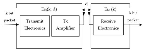
Figure 1. Radio energy model.

Equation (2) shows the energy spent in data transmission:

$$E_T (l, d) = \{\begin{array}{l}{E}_{elec} \ast l + E_{fs } \ast l \ast d^2 if d < d_0\\ E_{elec} \ast l + E_{mp} \ast l \ast d^4 if d \ge d_0\end{array}$$

(2)

where d and l are distance measurement value and data size, respectively.

Equation (3) expresses the energy spent on receiving purposes:

$$E_R = E_{elec} \ast l$$

(3)

where E_elec is the value of energy to run the electronic circuitry, and E_fs, and E_mp stand for free-space amplifier energy and multipath amplifier energy, respectively.

Equation (4) illustrates the threshold value of distance (d₀):

$$d_0 = \sqrt{\frac{E_{fs}}{E_{mp}}}$$

(4)

4. Proposed Algorithm

Clustering preserves the energy expenditure of the network. A single combination of input parameters does not decide CHs properly, resulting in network performance and lifetime degradation. The proposed protocol (FFMCP) defines and further uses a different set of parameters relevant for CH selection. FFMCP improves the performance by using multiple combinations of input parameters for CH nomination. Consider the hierarchy of two levels for data routing and assume that the first level performs CH selection and the second layer handles the task of data routing. After sensing the environmental data, member nodes send data to the CH for onward transmission to the BS. FFMCP considers the modalities of a fuzzy inference system (FIS) to define the complete working properly.

Fuzzy logic is used for the decision-making of unclear events; the results of these events can not be labeled “yes” and “no” or “true” and “false”. It mimics the decision-making of humans; there may be possible outcomes between “yes” and “no”. It primarily consists of four modules, shown in Figure 2 below:

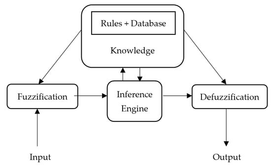
Figure 2. Fuzzy logic system.

Fuzzification: in this module, crisp input is transformed in to fuzzy sets based on linguistic terms. Each variable of linguistics is quantified by the membership function, to determine the suitable range of input.

Knowledge: this module consists of rule-based knowledge that is provided by the experts or a rigorous evaluation of the set of linguistic rules. It requires database knowledge for determining control and management rules.

Inference Engine: it has a function for determining the true value and rules to interpret the reasoning, for “if-then” logic. As an example, if the energy of the sensor node is high, then there is a strong probability for this sensor node to be the CH.

Defuzzification: the module transforms fuzzy sets acquired from the inference engine in to crisp output values, having proper weight with the center of gravity.

The execution of the protocol takes place for a predefined number of rounds. Two different combinations of input-output parameters are responsible for CH selection. Table 1 and Table 2 describe the input variables, output variables, and relationships among variables required for chance value calculations. FFMCP uses multiple chance values during the CH selection process.

Table 1. Fuzzy “if-then” mapping rule for chance 1.

Residual Energy	Count	Chance 1
Low	Low	Verylow
Medium	Low	Low
High	Low	Medium
Low	Medium	Low
Medium	Medium	Medium
High	Medium	Medium
Low	High	Medium
Medium	High	High
High	High	Veryhigh

Table 2. Fuzzy “if-then” mapping rule for chance 2.

Residual Energy	MCH	Chance 2
Low	Far	Very small (VS)
Medium	Far	Small (S)
High	Far	Rather small (RS)
Low	Medium	Mediumsmall (MS)
Medium	Medium	Medium (M)
High	Medium	Mediumlarge (ML)
Low	Close	Ratherlarge (RL)
Medium	Close	Large (L)
High	Close	Verylarge (VL)

4.1. Opening Phase

The opening phase consists of three major sections. The first phase deals with information collection and sharing, the second phase performs distance calculation, and the third phase performs degree and range calculation.

4.1.1. Information Collection and Sharing

Nodes are deployed randomly in WSNs and should share the location and other information with neighboring nodes. Sensor nodes broadcast messages to inform the location and working characteristics of the proposed protocol.

4.1.2. Distance Calculation

After the node’s deployment in the region of interest, BS broadcasts the message to evaluate the BS distance from sensor nodes. The signal strength indicator is the parameter to perform distance calculation of sensor nodes. The difference of distance from the BS gives input to calculate the distance between two sensor nodes. The following equation shows the distance evaluation:

$$d_z = \left|d_a - d_b\right|$$

(5)

where d_z is the distance between two nodes, and d_a and d_b are the maximum and minimum distances of a node from BS, respectively.

4.1.3. Degree and Range Calculation

The degree of a node tells about the neighbor density of a sensor node and has significant importance. Further range of each sensor node is as shown below:

$$C{R}_i (S_i) = (1-q \times \left(\frac{M{A}_d - DBS(S_i)}{M{A}_d -M{I}_d}\right) \times R)$$

(6)

where R = range, q = constant parameter, MI_d = the minimum distance of a sensor node from BS, MA_d = the maximum distance of a sensor node from BS, and DBS (S_i) = distance of a sensor node from BS.

4.2. Set-Up Phase

The set-up phase works in four parts. The first part is responsible for the node’s information advertisement, the second performs tentative CH selection, the third carries out final CH selection, and the fourth part handles cluster formation.

4.2.1. Advertisement Phase

The different information of a sensor node is distributed to the neighboring nodes in the advertisement phase. Each sensor node broadcasts three parameters, namely ID, competition radius, and sensor energy to other nodes in the communication range and finally decides the tentative CHs. Each sensor node maintains two separate tables for retaining network information. The first table maintains the self-information of each node while the second table keeps the information of the other neighboring nodes. Self attributes of a node are location, range, and ID of a node.

4.2.2. Tentative CH Selection Phase

We apply a fuzzy C-mean clustering approach to select the tentative CH nodes [43]. Each sensor node has some membership value in all the clusters; a sensor can belong to every group with a different membership value. For every sensor, the total sum of the membership value of all the clusters is 1. Membership value depends on the distance between cluster centroid and data point. The lesser the distance value is, the higher the membership value, and vice-versa.

C = {c₁, c₂, …… c_k} is the set of the centroids of k number of clusters, U = {µ_ij}_n*k is membership matrix and µ_ij is the membership degree to which observation i^th node p_i belongs to cluster having a centroid c_i. The aim is to minimize the objective function present in Equation (7) by FCM technique:

$$J (U, C) = {{\displaystyle \sum _{j=1}^k{\displaystyle \sum _{i=1}^n{\mu }_{ij}^m \Vert p_i - c_i\Vert }}}^2$$

(7)

where ${{\displaystyle \sum }}_{j=1}^K{\mu }_{ij}=1\forall \mathrm{i}$, m is a fuzzifier that is constant and controls the degree of fuzziness; it ranges between 1 < m < $\infty$. The degree of membership for the i^th node in j^th cluster is calculated by Equation (8).

$${\mu }_{ij} = {\left[{{\displaystyle \sum _{q=1}^K\left(\frac{\Vert p_i - c_j\Vert }{\Vert p_i - c_q\Vert }\right)}}^{\frac{2}{m-1}}\right]}^{-1}$$

(8)

The centroid point of each cluster in iteration is updated and is calculated by Equation (9).

$$\lceil {\displaystyle \sum _{i=1}^n{\mu }_{ik}^m P_k}\rceil$$

(9)

4.2.3. Final CH Selection Phase

Algorithm 1 describes the detailed working of the FFMCP method. The inputs of Algorithm 1 are the number of rounds (n_round), deployment area, probability, the position of the sink (sink_p), the initial energy of nodes (initial_e), range (c_range), number of nodes (n_nodes), and type of nodes (t_node). The outputs of Algorithm 1 are a set of CHs and a set of alive nodes. Line1 performs parameter initialization. FFMCP executes for n_round rounds. In each execution round, Algorithm 1 uses the degree and competition range for different types of evaluations. Lines 4–8 perform to check for alive nodes. The proposed algorithm utilizes two different combinations of input-output parameters for the CH chance value. Rounds 4, 7, 11, … consider residual energy and count of tentative CH nodes to calculate the chance value. Rounds 2, 5, 8, … do not perform the CH selection and uses the alive CHs of the previous round. Rounds 3, 6, 9, … use the energy and nearest CH distance to calculate the CH chance value. Nodes perform maximum energy saving since FFMCP consider energy in each round for CH chance value calculation. Initial CHs are selected using the fuzzy C-mean (FCM) clustering approach in round 1. Lines 3–25 and lines 29–46 show pseudo-code for first clustering and second clustering. In lines 26–28, data transmission takes place using previous alive CHs. The design of fuzzy inference system and defuzzification method is carried out using the Mamdani inference system. Figure 3 shows the detailed working of Algorithm 1. Each round of Algorithm 1 selects CHs based on fuzzy input parameters.

Algorithm 1: FFMCP Algorithm

Input: n_round, deployment area, p, sink_p, initial_e, c_range, n_nodes, t_node Output: R_VALUE={CHs, alive_n} 1: Initialization; 2: for r = 1 to n_round 3: if (mod(r,3) == 1) 4: for I = 1 to n 5:                  if(S(i).energy <= 0) 6:                               alive = alive − 1; 7:                   end if 8: end for 9: SAY_ HI_MESSAGE (ID, CR, SE) 10: if r = 1 11: apply FCM algorithm to select the initial tentative CHs 12: end if 13: if r > 1 14: S(i).chance1 = evalfis ([S(i).energy S(i).count_tch], z); 15: end if 16: if(S(i) = best(chance1) 17:                               S(i).t_node = TCH; 18: CONFIRM_TCH_MESSAGE (ID) 19: end if 20: if (S(i).E < S(j).E) 21: S(i).type = N; 22: end if 23: Nodes with S(i).t_node =TCH will be declared final CH 24: MEMBER_JOIN_CH_MESSAGE(ID) 25: End if 26: if (mod(r,3) == 2) and previous CHs are alive 27: transmit the date to the CH 28: else select the best chance CH 29: if (mod(r,3) == 0) 30: for I = 1 to n 31:                  if(S(i).energy <= 0) 32:                               alive = alive − 1; 33:                   end if 34: end for 35: SAY_ HI_MESSAGE (ID, CR, SE) 36: S(i).chance2 = evalfis ([S(i).energy S(i).mch], z); 37: if(S(i) = best(chance2) 38:                               S(i).t_node = TCH; 39: CONFIRM_TCH_MESSAGE (ID) 40: end if 41: if (S(i).E < S(j).E) 42: S(i).type = N; 43: end if 44: Nodes with S(i).t_node = TCH will be declared final CH 45: MEMBER_JOIN_CH_MESSAGE(ID) 46: end if 47: end for 48: Return R_VALUE

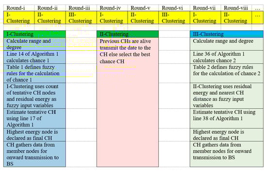
Figure 3. Detailed explanation of Algorithm 1.

Figure 4, Figure 5, Figure 6, Figure 7 and Figure 8 show the membership function of the node’s remaining energy, tentative CH count, minimum distance to CH, chance 1, and chance 2 values, respectively.

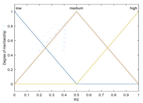
Figure 4. Membership function for residual energy.

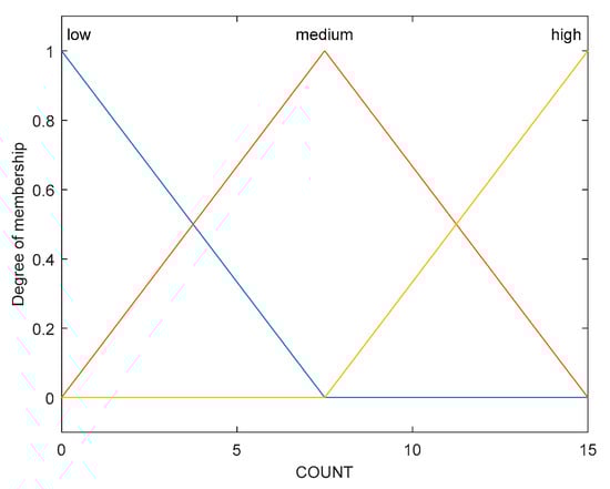
Figure 5. Membership function for count.

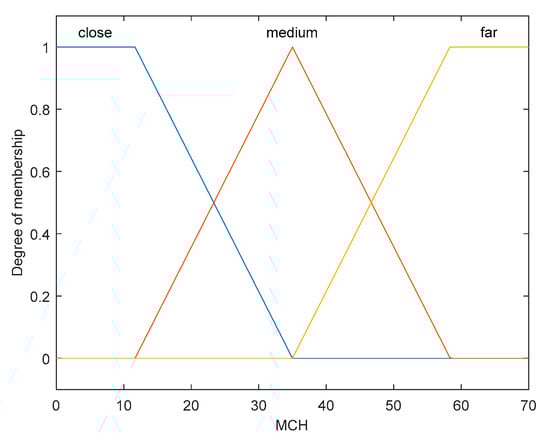
Figure 6. Membership function for min CH distance.

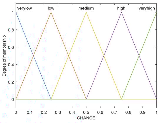
Figure 7. Membership function for chance 1.

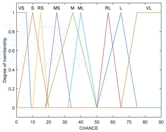
Figure 8. Membership function for chance 2.

Each node calculates chance value using the rules of Table 1 and Table 2 and further finalizes CHs with maximum chance value.

Due to uncertainty, FIS supports selecting the CHs whose fitness value is superior. FIS development took place to perform the CH selection and supervise the member nodes to join the suitable CH. The key benefit of the FIS is the low computational complexity. FFMCP selects CHs having a higher chance value in a particular round of algorithms.

The range of input variables for residual energy, count of tentative CHs, and minimum distance to CH is (0, 1), (0, 15), and (0, 70), respectively. The range of output variables for chance 1 and chance 2 is (0, 1) and (0, 100) respectively. The linguistic variables of the input values (RE, COUNT) are low, medium, and high; linguistic variables of the input value (MCH) are close, medium, and far. The linguistic variables of the output value (chance 1) are very low, low, medium, high, and very high; linguistic variables of the output value (chance 2) are very small, small, rather small, medium small, medium, medium large, rather large, large, and very large.

Inference engine based on fuzzy logic: it is complex and difficult to design a mathematical model for a changing WSN scenario. It is not easy to extend the mathematical model, which is designed for static WSN scenarios and can cater to some specific requirements. The value of environmental variables changes frequently, so the WSN deployment scenario becomes more dynamic. Energy, proximity, and inter-node distance are popular variables for controlling and monitoring different WSN scenarios. A fuzzy inference engine supports the uncertainty management of monitoring variables and enhances the accuracy of the results. Fuzzy rule-based systems are significant because of the approximate reasoning when there is a degree of uncertainty and imprecision in the data in the reasoning process. Membership functions are inputs and fuzzy rules perform decision-making for the inference engine.

Membership functions: membership functions show the truth degree of the variables (input/output) and represent quantitative measures through a set of vaguely defined values. The tuning of the membership function and reduction in system design time occurs for parameterizable functions. The optimization of parameters for proper CH selection requires time and computational cost. FFMCP performs several simulations to finalize the input parameter’s membership functions. For example, intersection points determine the peak value of the membership function. Membership function tuning takes place with the help of fuzzy results to cover the desired situation. In FFMCP, some membership functions are modified due to the uncertainty of parameters. Proposed work performs simulation rounds and considers network size and node density to tune the membership function. Triangular and trapezoidal membership functions are easy for tuning and suitable to handle network dynamism. The change in the parameter’s value is directly related to the desired changes in the two membership functions.

“If-then” rules: there is a set of linguistic rules to map the input parameters with output parameters as given by:

IF X, THEN Y, X represents a group of input parameters (energy level, degree, distance) and connections (NOT, OR, AND), and Y represents a group of output variables (chance value). We have two different combinations of input-output variables. In each group, there are two inputs and one output variable. The output variable corresponds to chance for CH. There are nine different rules in each case to control the uncertainty.

The defuzzification is based on the center of area (COA) method to calculate the crisp value.

Trapezoidal membership function (Equation (10)) is applied for boundary variables and triangular membership function (Equation (11)) for intermediate variables.

$${\mu }_A(x) = f(x) = \{\begin{array}{l}0, (x< a) \parallel (x > d)\\ \frac{x-a}{b-a} , a \le x \le b\\ 1 , b \le x \le c\\ \frac{d-x}{d-c} , c \le x \le d\end{array}$$

(10)

$${\mu }_A(x) = f(x) = \{\begin{array}{l}0, x\le a\\ \frac{x-a}{m-a} , a < x \le m\\ \frac{b-x}{b-m} , m < x <b\\ 0 , x \ge b\end{array}$$

(11)

4.2.4. Cluster Formation Phase

Each node selects the nearest CH and forms the cluster by broadcasting the message in the competition range using a non-persistent carrier sense multiple access (CSMA) MAC. The message announcement contains the ID of the CH. After receiving the message, sensor nodes finalize suitable CH for cluster formation. The smaller the communication range, the smaller the cluster size will be, saving the energy efficiently. Once the cluster formation completes, CH performs data collection from the cluster member using the TDMA schedule. TDMA execution performs with the help of members of the CH. TDMA also controls the collision during data transmission. It schedules the member nodes using the sleep-wake protocol; member nodes will save energy by going to a sleep state once the data transmission work finishes.

4.3. Data Transmission Phase

Data transmission takes place after the set-up phase finishes execution. CH uses the TDMA schedule to transmit data to the BS. Multiple communications take place during data transmission. Cluster members send data to the CH via intra-cluster communication and CHs collect the data. The data collected by the CH is further transmitted to the BS via inter-cluster communication.

Equation (12) approximates total energy usage for the cluster formation (EC_intra) and the multihop (EC_inter) transmitting to BS in one complete round.

$$E_{tot} = E{C}_{\mathrm{int}ra} +E{C}_{\mathrm{int}er}$$

(12)

The EC_intra includes the energy used in transmitting from cluster member to its CH (ECH_member), energy used to receive data at CH (ECH_receive), and also data aggregate (E_DA) from all its members for forwarding purposes. It can be shown in Equation (13) as:

$$E{C}_{\mathrm{int}ra} = EC{H}_{member} + EC{H}_{receiver} + N \times E_{DA}$$

(13)

$$EC{H}_{member} = {\displaystyle \sum _{j=1}^N{E}_{T_X} (k, C{M}_j , CH)}$$

(14)

$$EC{H}_{receiver} = N \times E_{R_X}(k)$$

(15)

The EC_inter only requires enough energy to forward information from all the CH through multiple hops to BS as in Equation (16):

$$\begin{array}{l}{EC}_{\mathrm{int}er} = E_{T_X}(k, CH,C{H}_1) + {\displaystyle \sum _{i=1}^m{E}_{T_X}}(k, C{H}_{i-1},C{H}_i) \\ + E_{T_X}(k, C{H}_m,BS) + m{E}_{R_X}\end{array}$$

(16)

Here, transmission order is from CH_i−1 to CH_i, with CH₁ as the initial CH of m intermediate CHs.

Time synchronization is an essential feature for the functioning of WSNs. Many pieces of research regarding time synchronization have been accomplished in recent years. Numerous protocols are proposed [44,45,46] for this problem. The clock of the sensor nodes should converge quickly to synchronize the different operations among sensor nodes. In [44], the author proposed three protocols for time synchronization, with a common goal of clock convergence. FFMCP protocol can use the protocol of [44] to perform the different operations in a synchronized manner; due to lesser message transmissions, this will save the energy of sensor nodes.

5. Comparative Analysis of Result and Simulation Work

Proper algorithm analysis and performance comparison in different network scenarios is the key aim of the simulation. All simulations for evaluation of performance carry out using the Matlab tool. The performance of FFMCP with that of LEACH, EAUCF, FLECH, DUCF, and EEFUC in terms of tenth node death (TND), half node death (HND), remaining energy after 800 rounds (E_800), and average energy spent per round (AVG_PR) is plotted in Figure 9, Figure 10, Figure 11 and Figure 12, respectively. Table 3, Table 4 and Table 5 show the quantitative details. Simulations perform in three different scenarios, considering the resultant value of the average of 10 different simulations in each case.

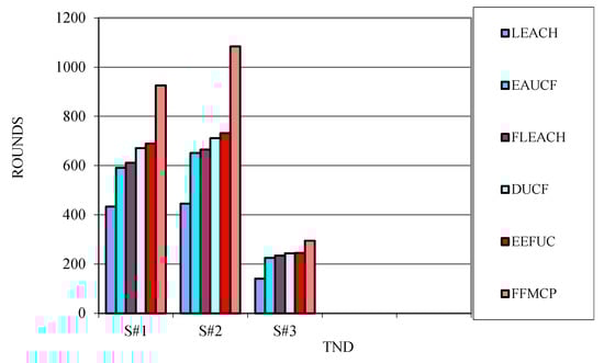
Figure 9. TND in different scenario.

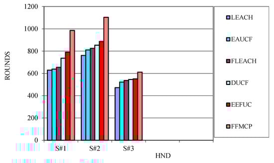
Figure 10. HND in different scenario.

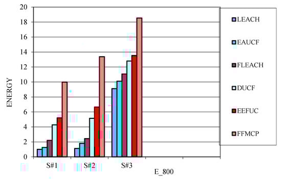
Figure 11. Residual energy after 800 round in a different scenario.

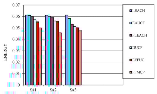
Figure 12. Average energy spent per round.

Table 3. Performance of scenario 1.

Algorithm	TND	HND	E_800	AVG_PR
LEACH	433	629	1.01	0.0612
EAUCF	591	639	1.26	0.0609
FLECH	611	665	2.21	0.0597
DUCF	671	737	4.28	0.0571
EEFUC	689	791	5.21	0.0553
FFMCP	926	985	9.98	0.0500

Table 4. Performance of scenario 2.

Algorithm	TND	HND	E_800	AVG_PR
LEACH	445	761	1.12	0.0611
EAUCF	651	811	1.81	0.0602
FLECH	665	825	2.44	0.0594
DUCF	711	854	5.15	0.0560
EEFUC	732	887	6.65	0.0559
FFMCP	1084	1103	13.38	0.0457

Table 5. Performance of scenario 3.

Algorithm	TND	HND	E_800	AVG_PR
LEACH	141	472	9.12	0.0612
EAUCF	225	522	10.11	0.0582
FLECH	234	537	11.06	0.0532
DUCF	244	546	12.8	0.0511
EEFUC	245	551	13.54	0.0501
FFMCP	295	611	18.54	0.0481

FFMCP establishes its importance and produces better results than other protocols (LEACH, EAUCF, FLECH, DUCF, and EEFUC). FFMCP discards the analysis for first node death and last node death. The network performance does not suffer much due to the death of a small number of nodes. The network performance decreases significantly after 50% of the nodes die. The simulation results analyze the effectiveness of FFMCP for the following three scenarios:

−

First scenario, S#1 (Figure 13) considers the network area of (200*200) with the base station located at (100, 100) and the initial energy of each node as 0.5 joules;

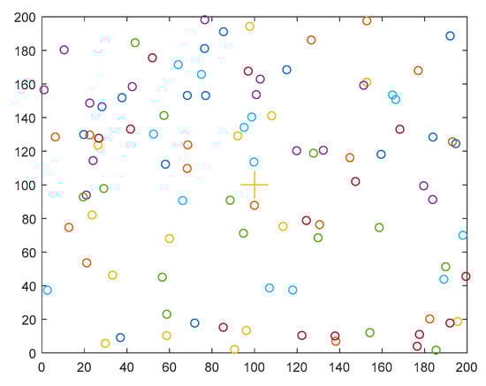Figure 13. First scenario.

−

Second scenario, S#2 (Figure 14) has an area of (100*100), base station location as (50, 50) initial energy of each node as 0.5 joules;

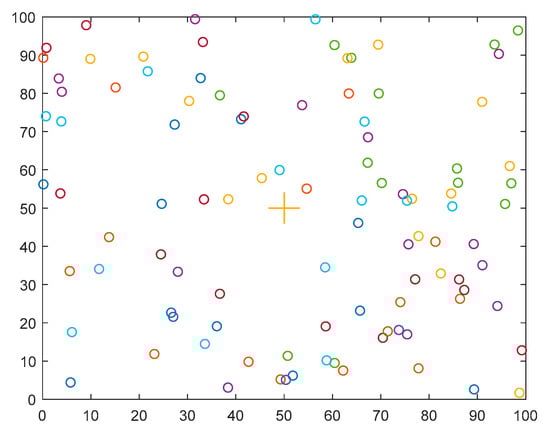Figure 14. Second scenario.

−

Third scenario, S#3 (Figure 15) has an area of (500*500), base station location as (500, 500) initial energy of each node as 5 joules.

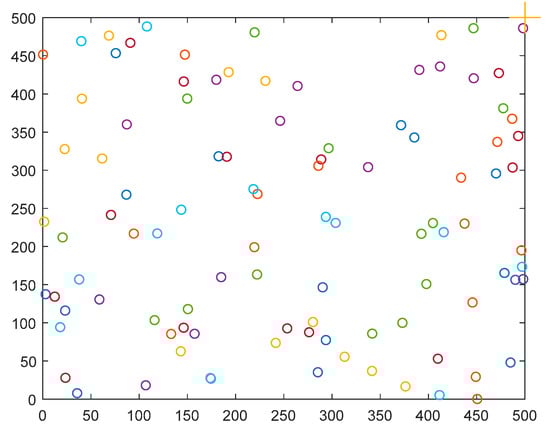Figure 15. Third scenario.

The other necessary parameters for our simulation to work in different scenarios are mentioned in Table 6. FFMCP always performs better than the other considered protocols.

Table 6. Parameters considered for simulations.

#Parameters	#Value
Nodes totality	100
Eelec	50 nJ/bit
Efs	10 pJ/bit/m2
Emp	0.0013 pJ/bit/m4
EDA	5 nJ/bit/message
Datasize	4000 bits
Control message	200 bits

Scenario 1: the deployment of 100 homogeneous (same initial energy) nodes in a large area (200*200) for reasonable comparison among protocols is considered. Table 3 demonstrates the performance of scenario1.

TND parameter is 113.9% better than LEACH, 56.7% better than EAUCF, 51.6% better than FLECH, 38% better than DUCF, and 34.4% better than EEFUC. HND parameters perform 56.6% better than LEACH, 54.1% better than EAUCF, 48.1% better than FLECH, 33.6% better than DUCF, and 24.5% better than EEFUC. The residual energy for FFMCP is eight times more than that of LEACH, seven times that of EAUCF, three times that of FLECH, twice that of DUCF, and 91.6% better than EEFUC for 800 rounds. The average energy spent per round for FFMCP is 18.3% less than LEACH, 17.9% less than EAUCF, 16.2% less than FLECH, 12.4% less than DUCF, and 9.6% less than EEFUC.

Scenario 2: its area is smaller (100*100) than scenario 1 but has the same initial energy. The purpose of this scenario is to analyze the behavior of the protocols for small area networks. The performance of the protocols is described in Table 4. FFMCP shows superiority over other protocols under consideration. Table 4 shows different performance-associated parameters in scenario 2. TND parameter is 143.6% better than LEACH, 66.5% better than EAUCF, 63% better than FLECH, 52.5% better than DUCF, and 48.1% better than EEFUC. HND parameters perform 44.9% better than LEACH, 36% better than EAUCF, 33.7% better than FLECH, 29.2% better than DUCF, and 24.4% better than EEFUC. The residual energy for FFMCP is much higher than other protocols for 800 rounds. The residual energy for FFMCP is 103.3% better than LEACH, 83.4% better than EAUCF, 67.6% better than FLECH, 44.8% better than DUCF, and 101.2% better than EEFUC. The average energy spent per round for FFMCP is 21.4% less than LEACH, 17.4% less than EAUCF, 9.6% less than FLECH, 5.9% less than DUCF, and 18.2% less than EEFUC.

Scenario 3: the area is more (500*500) as compared to scenario 1 and scenario 2. The initial energy is also larger than the other two scenarios. The purpose of this scenario is to analyze the behavior of the protocols for large area net works. The performance of the protocols exists in Table 5. FFMCP shows superiority over other protocols under consideration. Table 5 shows different performance-associated parameters in scenario 3. TND parameter is 109.2% better than LEACH, 31% better than EAUCF, 26.1% better than FLECH, 20.9% better than DUCF, and 20.4% better than EEFUC. HND parameters perform 29.5% better than LEACH, 17.1% better than EAUCF, 13.8% better than FLECH, 11.9% better than DUCF, and 10.9% better than EEFUC. The residual energy for FFMCP is much higher than other protocols for 800 rounds. The average energy spent per round for FFMCP is 25.2% less than LEACH, 24.1% less than EAUCF, 23.1% less than FLECH, 18.4% less than DUCF, and 3.9% less than EEFUC.

The simulation work reveals that the FFMCP protocol performs better than other protocols for tenth node death (TND), half node death (HND), and remaining energy after 800 rounds (E_800), and average energy spent per round (AVG_PR). The parameters used for the performance evaluation are popular for WSN clustering. The network performance decreases as the node’s energy reduces below a threshold limit. After 10% of nodes die, the network performance hampers significantly. Data collection and aggregation suffer a lot after 50% of nodes die. The higher the value of remaining energy after a certain round of algorithm execution, the more useful is the protocol for the real-time scenario. Table 1 and Table 2 define fuzzy rules for cluster head selection. Each rule considers energy as one parameter. The rule-based fuzzy system controls the energy expenditure of sensor nodes; as a result, the average energy spent per round is the lowest for the proposed protocol. The FFMCP protocol shows a better scalability feature, as it shows significant performance gain in a large-scale scenario.

FFMCP runs a pre-defined number of rounds to draw a box plot. Figure 16, Figure 17 and Figure 18 show the box plot of the proposed protocol for three different scenarios (S#1, S#2, S#3). The box plots represent the energy distribution of 100 sensor nodes.

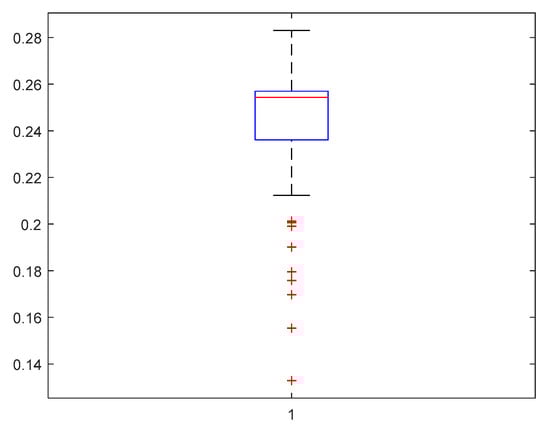
Figure 16. Box plot of node’s energy distribution in S#1.

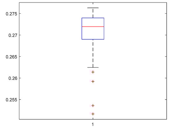
Figure 17. Box plot of node’s energy distribution in S#2.

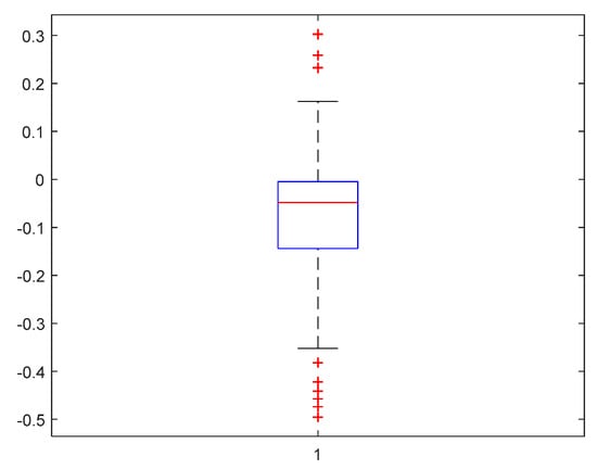
Figure 18. Box plot of node’s energy distribution in S#3.

6. Conclusions and Future Works

Network information of the previous round helps in predicting the better CH for the next round. The proposal (FFMCP algorithm) is a feed-forward multi-clustering protocol. FFMCP uses a fuzzy inference system to overcome the uncertainties in the value of input parameters. The proposed protocol calculates chance value by using two different sets of input parameters. FFMCP performance is better than the other protocols, as it considers the information of the previous round to calculate the chance value. Residual energy, tentative CH count, and minimum distance to CH facilitate to calculate output parameters. FFMCP shows enhanced performance than LEACH, EAUCF, FLECH, DUCF, and EEFUC in each case.

In the future, an analysis of the performance assuming some extraordinary energy harvesting nodes is probable research scope. Node deployment is in a square area; another deployment pattern is also possible. Simulations run for the stable sink, so controlled or pre-determined mobility can also be a future work. More discussions can take place on the number of mobile sensor nodes and their positions.

References

- Chen, Y.-C.; Wen, C.-Y. Distributed Clustering With Directional Antennas for Wireless Sensor Networks. IEEE Sens. J. 2013, 13, 2166–2180. [Google Scholar] [CrossRef]
- Babaie, S.; Zadeh, A.K.; Amiri, M.G. The New Clustering Algorithm with Cluster Members bounds for energy dissipation avoidance in wireless sensor network. In Proceedings of the 2010 International Conference On Computer Design and Applications, Qinhuangdao, China, 25–27 June 2010; Volume 2, pp. V2-613–V2-617. [Google Scholar]
- Mishra, P.K.; Verma, S.K. A survey on clustering in wireless sensor network. In Proceedings of the 2020 11th International Conferenceon Computing, Communication and Networking Technologies (ICCCNT), Kharagpur, India, 1–3 July 2020; pp. 1–5. [Google Scholar]
- Kaur, R.; Sharma, M. An approach to design habitat monitoring system using sensor networks. Int. J. Soft Comput. Eng. 2011, 1, 5–8. [Google Scholar]
- Suzuki, M.; Saruwatari, S.; Kurata, N.; Morikawa, H. A high-density earth quake monitoring system using wireless sensor networks. In Proceedings of the 5th International Conference on Bioinformatics and Computational Biology; Association for Computing Machinery: New York, NY, USA, 2007; pp. 373–374. [Google Scholar]
- Winkler, M.; Street, M.; Tuchs, K.D.; Wrona, K. Wireless sensor networks for military purposes. In Autonomous Sensor Networks; Springer: Berlin/Heidelberg, Germany, 2012; pp. 365–394. [Google Scholar]
- Winkler, M.; Tuchs, K.D.; Hughes, K.; Barclay, G. Theoretical and practical aspects of military wireless sensor networks. J. Telecommun. Inf. Technol. 2008, 2, 37–45. [Google Scholar]
- Ko, J.; Lim, J.H.; Chen, Y.; Musvaloiu, E.R.; Terzis, A.; Masson, G.M. MEDiSN:Medical emergency detection in sensor networks. Acm Trans. Embed. Comput. Syst. 2010, 10, 11. [Google Scholar] [CrossRef]
- Woznowski, P.; Burrows, A.; Diethe, T.; Fafoutis, X.; Hall, J.; Hannuna, S.; Camplani, M.; Twomey, N.; Kozlowski, M.; Tan, B.; et al. SPHERE: A Sensor Platform for Health care in a Residential Environment. In Designing, Developing, and Facilitating Smart Cities; Springer Science and Business Media LLC: Berlin/Heidelberg, Germany, 2016; pp. 315–333. [Google Scholar]
- Rashid, B.; Rehmani, M.H. Applications of wireless sensor networks for urban areas: A survey. J. Netw. Comput. Appl. 2016, 60, 192–219. [Google Scholar] [CrossRef]
- Ceriotti, M.; Mottola, L.; Picco, G.P.; Murphy, A.L.; Guna, S.; Corra, M. Monitoring heritage buildings with wireless sensor networks: The torreaquila deployment. In Proceedings of the 2009 International Conference on Information Processing in Sensor Networks, San Francisco, CA, USA, 13–16 April 2009; pp. 277–288. [Google Scholar]
- Dong, Q.; Yu, L.; Lu, H.; Hong, Z.; Chen, Y. Design of Building Monitoring Systems Based on Wireless Sensor Networks. Wirel. Sens. Netw. 2010, 2, 703–709. [Google Scholar] [CrossRef]
- Stojkoska, B.L.R.; Trivodaliev, K.V. A review of Internet of Things for smart home: Challenges and solutions. J. Clean. Prod. 2017, 140, 1454–1464. [Google Scholar] [CrossRef]
- Suryadevara, N.K. Wireless sensor sequence data model for smart home and IoT data analytics. In Proceedings of the First International Conference on Computational Intelligence and Informatics; Springer: Berlin/Heidelberg, Germany, 2017; pp. 441–447. [Google Scholar]
- Kafi, M.A.; Challal, Y.; Djenouri, D.; Doudou, M.; Bouabdallah, A.; Badache, N. A Study of Wireless Sensor Networks for Urban Traffic Monitoring: Applications and Architectures. Procedia Comput. Sci. 2013, 19, 617–626. [Google Scholar] [CrossRef]
- Liu, X.-Y.; Zhu, Y.; Kong, L.; Liu, C.; Gu, Y.; Vasilakos, A.V.; Wu, M.-Y. CDC: Compressive Data Collection for Wireless Sensor Networks. IEEE Trans. Parallel Distrib. Syst. 2014, 26, 2188–2197. [Google Scholar] [CrossRef]
- Heinzelman, W.B.; Chandrakasan, A.P.; Balakrishnan, H. An application-specific protocol architecture for wireless microsensor networks. IEEE Trans. Wirel. Commun. 2002, 1, 660–670. [Google Scholar] [CrossRef]
- Zahedi, A.; Arghavani, M.; Parandin, F.; Arghavani, A. Energy Efficient Reservation-Based Cluster Head Selection in WSNs. Wirel. Pers. Commun. 2018, 100, 667–679. [Google Scholar] [CrossRef]
- Deepa, C.; Latha, B. HHSRP: A cluster based hybrid hierarchical secure routing protocol for wireless sensor networks. Clust. Comput. 2017, 2, 1–17. [Google Scholar] [CrossRef]
- Huang, J.; Hong, Y.; Zhao, Z.; Yuan, Y. An energy-efficient multi-hop routing protocol based on grid clustering for wireless sensor networks. Clust. Comput. 2017, 20, 3071–3083. [Google Scholar] [CrossRef]
- Maddali, B.K. Core network supported multicast routing protocol for wireless sensor networks. IET Wirel. Sens. Syst. 2015, 5, 175–182. [Google Scholar] [CrossRef]
- Mohammed, T.; Kemal, E.T.; Sasan, A.; Shervin, E. Survey of multi path routing protocols for mobile adhoc networks. J. Netw. Comput. Appl. 2009, 32, 1125–1143. [Google Scholar]
- Du, R.; Chen, C.; Yang, B.; Lu, N.; Guan, X.; Shen, X. Effective Urban Traffic Monitoring by Vehicular Sensor Networks. IEEE Trans. Veh. Technol. 2015, 64, 273–286. [Google Scholar] [CrossRef]
- Younis, O.; Fahmy, S. HEED: A hybrid energy-efficient, distributed clustering approach for adhoc sensor networks. IEEE Trans. Mob. Comput. 2004, 3, 366–379. [Google Scholar] [CrossRef]
- Hoang, D.C.; Yadav, P.; Kumar, R.; Panda, S.K. Real-Time Implementation of a Harmony Search Algorithm-Based Clustering Protocol for Energy-Efficient Wireless Sensor Networks. IEEE Trans. Ind. Inform. 2013, 10, 774–783. [Google Scholar] [CrossRef]
- Demigha, O.; Hidouci, W.-K.; Ahmed, T. On Energy Efficiency in Collaborative Target Tracking in Wireless Sensor Network: A Review. IEEE Commun. Surv. Tutor. 2012, 15, 1210–1222. [Google Scholar] [CrossRef]
- Zhou, H.; Liu, B.; Luan, T.H.; Hou, F.; Gui, L.; Li, Y.; Yu, Q.; Shen, X. Chain Cluster: Engineering a Cooperative Content Distribution Framework for Highway Vehicular Communications. IEEE Trans. Intell. Transp. Syst. 2014, 15, 2644–2657. [Google Scholar] [CrossRef]
- Xu, Z.; Chen, L.; Chen, C.; Guan, X. Joint Clustering and Routing Design for Reliable and Efficient Data Collection in Large-Scale Wireless Sensor Networks. IEEE Internet Things J. 2015, 3, 520–532. [Google Scholar] [CrossRef]
- Heinzelman, W.R.; Chandrakasan, A.; Balakrishnan, H. Energy-efficient communication protocol for wireless micro sensor networks. In Proceedings of the 33rd Annual Hawaii International Conference on System Sciences, Maui, HI, USA, 7 January 2000; p. 8020. [Google Scholar]
- Manjeshwar, A.; Agrawal, D. TEEN: A routing protocol for enhanced efficiency in wireless sensor networks. In Proceedings of the 15th International Parallel and Distributed Processing Symposium, San Francisco, CA, USA, 23–27 April 2001; pp. 2009–2015. [Google Scholar]
- Bagci, H.; Yazici, A. An energy aware fuzzy approach to unequal clustering in wireless sensor networks. Appl. Soft Comput. 2013, 13, 1741–1749. [Google Scholar] [CrossRef]
- Balakrishnan, B.; Balachandran, S. FLECH: Fuzzy logic based energy efficient clustering hierarchy for non-uniform wireless sensor networks. Wirel. Commun. Mob. Comput. 2017, 1214720. [Google Scholar] [CrossRef]
- Baranidharan, B.; Santhi, B. DUCF: Distributed load balancing Unequal Clustering in wireless sensor networks using Fuzzy approach. Appl. Soft Comput. 2016, 40, 495–506. [Google Scholar] [CrossRef]
- Phoemphon, S.; So-In, C.; Aimtongkham, P.; Nguyen, T.G. An energy-efficient fuzzy-based scheme for unequal multi hop clustering in wireless sensor networks. J. Ambient. Intell. Hum. Comput. 2021, 12, 873–895. [Google Scholar] [CrossRef]
- Boubiche, S.; Boubiche, D.E.; Bilami, A.; Toral-Cruz, H. Big Data Challenges and Data Aggregation Strategies in Wireless Sensor Networks. IEEE Access 2018, 6, 20558–20571. [Google Scholar] [CrossRef]
- Dwivedi, A.; Sharma, A. FEECA: Fuzzy based Energy Efficient Clustering Approach in Wireless Sensor Network. ICST Trans. Scalable Inf. Syst. 2018, 7. [Google Scholar] [CrossRef]
- Hidoussi, F.; Toral-Cruz, H.; Boubiche, D.E.; Martínez-Peláez, R.; Velarde-Alvarado, P.; Barbosa, R.; Chan, F. PEAL: Power Efficient and Adaptive Latency Hierarchical Routing Protocol for Cluster-Based WSN. Wirel. Pers. Commun. 2017, 96, 4929–4945. [Google Scholar] [CrossRef]
- Sert, S.A.; Alchihabi, A.; Yazici, A. A Two-Tier Distributed Fuzzy Logic Based Protocol for Efficient Data Aggregation in Multihop Wireless Sensor Networks. IEEE Trans. Fuzzy Syst. 2018, 26, 3615–3629. [Google Scholar] [CrossRef]
- Lee, J.-S.; Teng, C.-L. An Enhanced Hierarchical Clustering Approach for Mobile Sensor Networks Using Fuzzy Inference Systems. IEEE Internet Things J. 2017, 4, 1095–1103. [Google Scholar] [CrossRef]
- ElAlami, H.; Najid, A. ECH: An Enhanced Clustering Hierarchy Approach to Maximize Lifetime of Wireless Sensor Networks. IEEE Access 2019, 7, 107142–107153. [Google Scholar] [CrossRef]
- ElAlami, H.; Najid, A. Energy-efficient fuzzy logic cluster head selection in wireless sensor networks. In Proceedings of the 2016 International Conference on Information Technology for Organizations Development (IT4OD), Fez, Morocco, 30 March–1 April 2016; pp. 1–7. [Google Scholar]
- Lee, J.-S.; Cheng, W.-L. Fuzzy-Logic-Based Clustering Approach for Wireless Sensor Networks using Energy Predication. IEEE Sens. J. 2012, 12, 2891–2897. [Google Scholar] [CrossRef]
- Su, S.; Zhao, S. An optimal clustering mechanism based on Fuzzy-C means for wireless sensor networks. Sustain. Comput. Inform. Syst. 2018, 18, 127–134. [Google Scholar] [CrossRef]
- Bruscato, L.T.; Heimfarth, T.; DeFreitas, E.P. Enhancing Time Synchronization Support in Wireless Sensor Networks. Sensors 2017, 17, 2956. [Google Scholar] [CrossRef] [PubMed]
- Zhang, D.; Yuan, Y.; Bi, Y. A Design of a Time Synchronization Protocol Based on Dynamic Route and Forwarding Certification. Sensors 2020, 20, 5061. [Google Scholar] [CrossRef]
- Wang, Z.; Zeng, P.; Zhou, M.; Li, D.; Wang, J. Cluster-Based Maximum Consensus Time Synchronization for Industrial Wireless Sensor Networks. Sensors 2017, 17, 141. [Google Scholar] [CrossRef] [PubMed]
Short Biography of Authors