Increased Internal Combustion Engine Efficiency with Optimized Valve Timings in Extended Stroke Operation

Abstract

Spark-ignited internal combustion engines are known to exhibit a decreased brake efficiency in part-load operation. Similarly to cylinder deactivation, the x-stroke operation presented in this paper is an adjustable form of skip-cycle operation. It is an effective measure to increase the efficiency of an internal combustion engine, which has to be equipped with a variable valve train to enable this feature. This paper presents an optimization procedure for the exhaust valve timings applicable to any valid stroke operation number greater than four. In the first part, the gas spring operation, during which all gas exchange valves are closed, is explained, as well as how it affects the indicated efficiency and the blow-by mass flow. In the second part, a simulation model with variable valve timings, parameterized with measurement data obtained on the engine test, is used to find the optimal valve timings. We show that in 12-stroke operation and with a cylinder load of 5 Nm, an indicated efficiency of 34.3% is achieved. Preloading the gas spring with residual gas prevents oil suction and thus helps to reduce hydrocarbon emissions. Measurements of load variations in 4-, 8-, and 12-stroke operations show that by applying an x-stroke operation, the indicated efficiency remains high and the center of combustion remains optimal in the range of significantly lower torque outputs.

1. Introduction

The automotive industry is under high political pressure to decrease its fleet average ${\mathrm{CO}}_2$ emissions. Effective as of the year 2020, the emission limit for new passenger cars is set by the European parliament to 95 $\mathrm{g}{\mathrm{CO}}_2$/$\mathrm{km}$, which corresponds to a gasoline consumption of 4.06 L/$100\mathrm{km}$. If the limit, averaged over the manufacturer’s complete fleet, is exceeded, sanctions must be paid. Similar measures are also applied to light- and heavy-duty commercial vehicles. In the future, these restrictions are tightened even further in order to achieve ${\mathrm{CO}}_2$ emission neutrality by 2050 [1,2,3,4]. A historical analysis of European emission limits is provided in [5]. The limitations currently in effect require novel solutions, since a modern passenger vehicle with a conventional internal combustion engine drive train is not capable of meeting the requirements [6].

Today, the majority of cars produced still relies on conventional internal combustion engines (ICE). Although hybridization of various degrees is becoming the new standard, neglecting technological advancement for ICEs would have a severe environmental impact. This is true especially when its importance for long-distance and heavy-duty applications is considered. For ICEs, it is crucial to maximize the thermal efficiency across their relevant operating range. Generally helpful for that purpose are any efforts to reduce the friction and weight of moving/rotating parts [7,8]. An increase of the compression ratio helps in improving the thermal efficiency, but is often limited by knock in the case of spark-ignited engines. Therefore, measures that reduce knock, such as direct injection or water injection, are useful [9,10,11]. In addition, the reduction of wall heat losses is beneficial, which can be achieved by innovative approaches, such as thermal swing coating of combustion chamber surfaces [12,13]. For passenger car applications with spark-ignited engines, many investigations focus on the part-load operating points, where the engine is operated often but the efficiency is usually poor if no special measures are taken. By applying Miller valve timings [14] (intake valves close early, that is, before bottom dead center) or Atkinson valve timings [15] (intake valves close late, that is, after bottom dead center) to control the cylinder charge instead of the conventional throttle, pumping losses are reduced [16]. Thus, the thermal efficiency is increased due to the extended expansion stroke relative to the compression stroke [17]. If a suitable exhaust aftertreatment system is used, lean combustion concepts with pre-chamber or pilot ignition lead to a significant increase of the thermal efficiency [18,19] and efficiency levels of above 45% are achievable for passenger car size engines [20]. Cooled exhaust gas recirculation in combination with variable compression ratios allows for improvement of the thermal efficiency, while the formation of emissions such as nitrogen-oxides (${\mathrm{NO}}_{\mathrm{x}}$) and hydrocarbons (HC) are decreased [21]. Another state-of-the-art method to increase part-load efficiency is cylinder deactivation, where a certain number of cylinders is disabled while the remaining cylinders continue operation at a higher load and, hence, at a higher thermal efficiency [22,23,24,25]. Measures that have been implemented for some time are downsizing and supercharging or electric boosting, which lead to a higher power density and increased efficiency [26,27,28,29]. Fuel efficiency further improves by use of start-stop systems, which have become standard equipment in the automotive sector [30]. Furthermore, with an electric motor present in the power train, a shift of the operating point is possible, leading to improved fuel economy [31,32]. As internal combustion engines are very likely to play an important role in future mobility, especially in long-distance applications, the decarbonization of fuel plays an important role. This can be done by biogenic or synthetic fuels. As the availability of renewable fuels is likely to be a challenge and the costs are expected to be higher than for fossil fuels, the future efforts for efficiency improvement will be driven by economic, rather than ecological reasons [33,34,35].

Another method to improve part-load efficiency is the skip-cycle strategy, also known as the skip-fire strategy, as investigated in [36,37,38,39]. With that method, one or more additional engine revolutions are executed after the regular four strokes, which leads to a lower frequency, but an increased load for each combustion instance. In [40], a skipped cycle is implemented after one or two consecutive fired cycles, which leads to a brake-specific fuel consumption reduction of 4.3% at a brake mean effective pressure of 1 bar. A reduction of fuel consumption by implementing one skipped cycle after each fired cycle is reported in [36], while a corresponding valve timing adaptation leads to a decrease in emissions. By applying the skip-cycle strategy together with an early intake valve opening, ${\mathrm{NO}}_{\mathrm{x}}$ emissions are reduced by up to 40% and, with a late exhaust valve opening, a reduction of HC emissions by up to 55% is achieved. In [41,42,43,44] skipped cycles are implemented dynamically, where it is decided on a cycle-by-cycle basis if a cylinder is fired or not. This also leads to an engine fuel consumption reduction, however, a sophisticated control algorithm is required to minimize vibrations induced by the uneven firing order. With the addition of an electric motor to the power train, vibrations induced by dynamic skip fire are reduced by almost 50%, as reported in [45]. Another benefit of the skip-cycle strategy is the increased exhaust gas temperature, which supports the exhaust aftertreatment system to reach and keep optimal operating conditions in situations such as cold-start or elongated low-load operations.

In this paper, we introduce a skip-cycle strategy where the conventional four-stroke cycle is extended by one or more additional engine revolutions. The choice of this number leads to new operation strategies as 6-, 8-, 10- or, as named in this paper in general, an x-stroke operation. These new strategies are compared to a strategy with cylinder deactivation using measurements obtained on the same engine. Similarly to cylinder deactivation, in x-stroke operation, the load of a single combustion is increased, but in contrast, all cylinders remain active. With an increasing number of strokes, the firing frequency is reduced. Thus, a low engine load is achieved with a high stroke number, which leads to a high specific cylinder charge for each combustion with high thermal efficiency. In contrast to the skip-cycle operations described above, the x-stroke operation runs steadily on all cylinders, and the cycle length is extendable such that even very low engine loads are realized at high thermal efficiency. In x-stroke operation, running the engine with deactivated valves results in a gas spring operation during the additional strokes. The transition from the conventional strokes into the gas spring operation and back has an impact on the indicated mean effective pressure (IMEP). However, it is not a priori clear how to actuate the gas exchange valves optimally such that the indicated efficiency is maximized. Furthermore, not only pumping losses have to be considered, but also a possible oil intake over the piston rings has to be minimized. In this paper, we show the effects of various exhaust valve timings during the x-stroke operation, similarly as in [46]. However, here, we analyze the gas spring operation during the additional strokes in detail, and we introduce a search routine to find the exhaust valve timings, which lead to the optimal indicated efficiency. A zero-dimensional model is used to gather data over a wide operating range for numerical optimization. An SI engine test bench, which is equipped with the fully variable valve train named FlexWork introduced in [47,48], is used to validate this model and the optimization procedure.

2. Setup of the Experiments

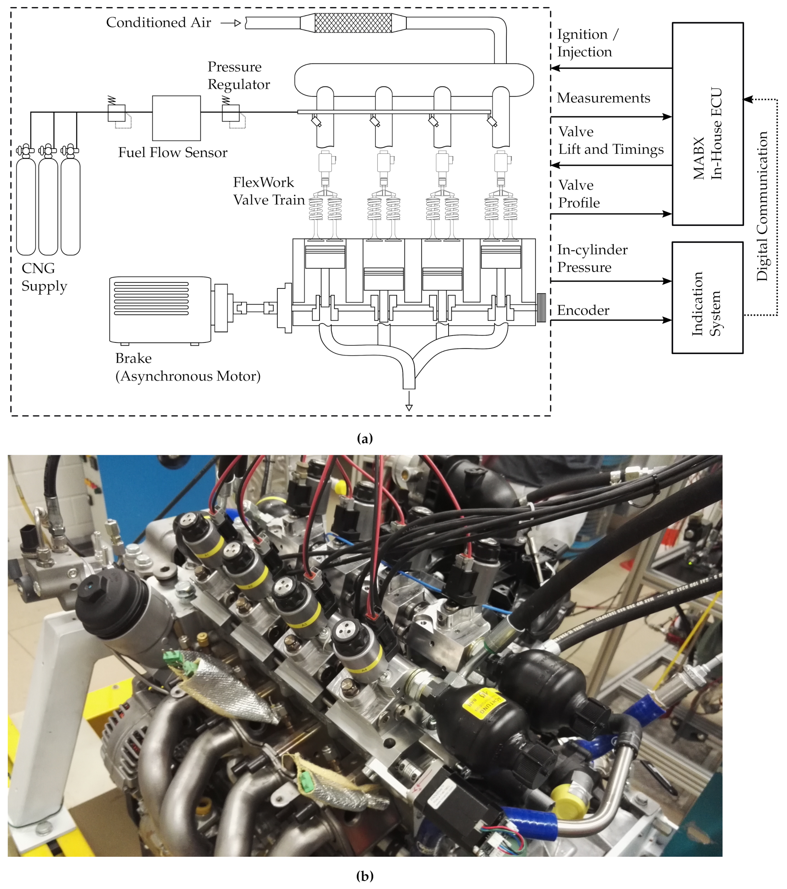
The engine used in this project is a 1.4 L Volkswagen spark-ignited engine of the type EA111. Originally, the engine is twin-charged with a mechanical compressor and a turbocharger. The engine control software is fully developed in-house and runs on a MicroAutoBoxII (MABX), which is a rapid prototyping system from dSPACE (Paderborn, Germany). The fuel used is natural gas with port-injectors, while the exhaust manifold is equipped with four lambda sensors to ensure the cylinder-individual feedback control for stoichiometric combustion. Furthermore, each cylinder is equipped with pressure transducers which are evaluated in real-time on the MABX such that the center of combustion (COC) is closed-loop controlled to be at 8 ${}^{\circ }$ crank angle (CA) after the top dead center (TDC). The original valve train—including intake and exhaust camshafts, gears, chains, and timing adjusters—was replaced by a fully variable electro-hydraulic valve train system called FlexWork. Our engine control software allows setting the valve timings of each cylinder individually. A detailed description of the equipment used is found in

Table 1. Details of the equipment used on the engine test bench.

Equipment	Details
Engine basis	Volkswagen EA111
Displacement	1.4 L, 4 cylinders
Bore/stroke	76.5 mm /75.6 mm
Compression ratio	10
Fueling	Port-injected CNG, NGI2 injectors (Bosch)
Valve train	FlexWork (internally developed)
Valve lift measurement	Linear encoders (Elgo Electronics)
Valve lift variability	1–9 mm, exhaust and intake
Valve timing variability	individual on all valve pairs
Engine control unit	MicroAutoBoxII (dSPACE)
Stoichiometry sensors	Wide band, LSU 4.9 (Bosch)
Fuel flow measurement	Coriolis sensor, RHM015 (Rheonik)
Combustion air flow measurement	Sensyflow P (ABB)
Blow-by measurement	Blow-by meter 4140/150 (AVL)
Torque measurement	HBM T40 torque transducer
Flywheel/gearbox	Standard dual mass/no gearbox

. An overview of the setup is shown in Figure 1.

FlexWork is a spring-mass system [49] which is hydraulically actuated and controlled by an electric solenoid valve. The two intake valves and the two exhaust valves of each cylinder are mechanically linked. Each cylinder is equipped with two solenoid valves. Hence, each valve pair can be actuated individually. Distinctive features are FlexWork’s low energy demand due to the automated hydraulic recuperation and its simplicity in design and control.

A detailed system description is presented in [17,48,50], and results of a fired engine operation are found in [16,47]. For the investigation in this paper, the following three features are relevant:

• For the intake and exhaust sides, the valve lift can be varied individually.
• For each valve pair on each cylinder, the valve timings can be set individually.
• For each engine cycle, the valve timings can be set individually.

These features allow the actuation of the intake valves and the number of openings of the exhaust valves to be adapted to the requested stroke number operation and optimal gas exchange. At a small valve lift, the valves can be opened while the piston is at TDC, which extends the range of possible valve actuation strategies.

3. Setup of the Simulation

A zero-dimensional process simulation serves to analyze the influence of different valve timings on the pressure progression inside the cylinder. The pressure and temperature in the intake manifold, exhaust manifold, and crankcase are kept constant. Furthermore, the intake manifold is assumed to be filled with a homogeneous, stoichiometric fuel/air mixture while the exhaust manifold contains only a homogeneous mixture of burned gas. To model the mass flow over the intake valves, exhaust valves, and piston rings the equations for compressible flows are used. All properties of the gases implemented, namely natural gas, air, and burned gas, are temperature-dependent and computed with NASA polynomials [51]. The heat released during combustion is described by the Vibe equation [52,53,54], while wall heat losses are accounted for by the Woschni correlation [54,55]. Coefficients for the Vibe function and the blow-by mass flow are validated by measurement data from the test bench.

3.1. Engine Parameters

In the simulation, the geometrical parameters of the VW EA111 engine are implemented according to Table 1. The focus of this paper lies in the influence of the exhaust valve timings on the IMEP. Cross-coupling effects between cylinders due to gas dynamics in the intake and exhaust manifolds are not considered. Hence, in this simulation, only one cylinder is modeled, which significantly reduces the computational effort.

Table 2. Constants applied in the process simulation.

Description	Unit	Value
Resolution	${}^{\circ }$CA	0.125
Ambient pressure	bar	$0.94$
Intake manifold pressure	bar	$0.94$
Exhaust manifold pressure	bar	$0.96$
Crankcase pressure	bar	$0.94$
Intake manifold temperature	K	300
Exhaust manifold temperature	K	600
Cylinder wall temperature	K	530
Intake valve lift	mm	1.9
Exhaust valve lift	mm	2.2
Blow-by area	${\mathrm{mm}}^2$	1.695
Stoichiometric air/fuel ratio	-	17.19
Lower heating value CNG	$\mathrm{MJ}$/$\mathrm{kg}$	48.529

shows an overview of the assumed constants.

The resolution is chosen to be as coarse as possible to increase computational performance, and as fine as required to prevent infeasible pressure oscillations in the Matlab solver. Pressure and temperature levels are average values obtained by measurements. The cylinder wall temperature is fitted such that the pressure progression during the gas-spring operation corresponds to the experimental data. The lift of the intake and exhaust valves corresponds to the settings used in the experiments. Since all experiments are conducted at a rather low rotational engine speed of 2000 rpm, the small valve lift is sufficient for the gas exchange. Furthermore, at such a small lift the valves can remain open even while the piston passes TDC. The blow-by area is fitted with blow-by measurement data obtained from a combination of supercharged, fired operation, and motored operation. The stoichiometric air/fuel ratio and the exact lower heating value for compressed natural gas (CNG) are determined by gas-phase chromatography.

3.2. Mass Flow

The mass flow in $(\mathrm{kg}/\mathrm{s})$ through the engine is controlled mainly by the timings of the intake and exhaust valves. Here the equation for compressible flows [56] is applied,

$$\dot{m}\left(t\right)=c_{\mathrm{d}}\left(t\right)·A\left(t\right)·\frac{p_{\mathrm{in}}\left(t\right)}{\sqrt{R·{\vartheta }_{\mathrm{in}}\left(t\right)}}·\Psi \left(\frac{p_{\mathrm{out}}\left(t\right)}{p_{\mathrm{in}}\left(t\right)}\right),$$

(1)

where, $\dot{m}$ is the mass flow, $c_{\mathrm{d}}$ is the valve’s discharge coefficient, and A is the geometrical area. The latter two both are depending on the valve lift, the variables $p_{\mathrm{in}}$ and $p_{\mathrm{out}}$ are the pressure upstream and downstream, respectively, while R is the specific gas constant, $\vartheta$ is the temperature, and $\Psi$ is the flow function, which is defined as

$$\Psi \left(\frac{p_{\mathrm{out}}\left(t\right)}{p_{\mathrm{in}}\left(t\right)}\right)=\{\begin{array}{cc}\sqrt{\kappa {\left[\frac{2}{\kappa +1}\right]}^{\frac{\kappa +1}{\kappa -1}}}\hfill & \mathrm{for}{p}_{\mathrm{out}}<p_{\mathrm{cr}},\\ {\left[\frac{p_{\mathrm{out}}}{p_{\mathrm{in}}}\right]}^{\frac{1}{\kappa }}·\sqrt{\frac{2·\kappa }{\kappa -1}·\left[1-{\left(\frac{p_{\mathrm{out}}}{p_{\mathrm{in}}}\right)}^{\frac{\kappa -1}{\kappa }}\right]}\hfill & \mathrm{for}{p}_{\mathrm{out}}\ge p_{\mathrm{cr}}.\end{array}$$

(2)

The variable $\kappa$ thus stands for the ratio of specific heats and $p_{\mathrm{cr}}$ is the critical pressure at which the flow reaches sonic conditions in the narrowest part, defined as

$$p_{\mathrm{cr}}={\left[\frac{2}{\kappa +1}\right]}^{\frac{\kappa }{\kappa -1}}·p_{\mathrm{in}}.$$

(3)

In the simulation the following two gas compositions are considered:

• Fresh mixture consisting of air (21% ${\mathrm{O}}_2$ and 79% ${\mathrm{N}}_2$) and ${\mathrm{CH}}_4$ at a stoichiometric ratio.
• Burned gas consisting of ${\mathrm{N}}_2$, ${\mathrm{CO}}_2$, and ${\mathrm{H}}_2\mathrm{O}$.

The gas fractions are computed depending on the inflow and outflow from and to both manifolds, blow-by losses, and the progression of the combustion. The intake manifold is assumed to be filled with a stoichiometric mixture of air and methane. However, if at the Intake Valve Opening (IVO), burned gas flows into the intake manifold, the burned gas is inducted back into the cylinder during the induction stroke before any fresh mixture enters the cylinder.

By design, piston rings create several small volumes to seal the cylinder from the crankcase against blow-by losses. To prevent the necessity of modeling the gas flow over each piston ring, the following procedure is applied: The engine is operated at a supercharged load point such that the cylinder pressure at all times is larger than the crankcase pressure, which leads to a constant positive blow-by mass flow, that is, from the cylinder into the crankcase. With (1) and the obtained measurement data, the blow-by area given in Table 2 is determined. Subsequently, the reverse flow, that is, from the crankcase into the cylinder, is analyzed. All valves are closed after the piston reaches TDC and the combustion chamber is approximately at ambient pressure. While the piston moves towards the bottom dead center (BDC), the pressure drops below ambient pressure and gas flows from the crankcase into the cylinder. The resulting in-cylinder pressure at BDC depends on the mass inducted from the crankcase. With these experiments, it is possible to fit a multiplicative correction factor $B{B}_{\mathrm{corr}}$ for the blow-by area, which is found to be

$$B{B}_{\mathrm{corr}}=\begin{array}{cc}0.26\hfill & \mathrm{for}{p}_{\mathrm{cyl}}<p_{\mathrm{crank}},\\ 1\hfill & \mathrm{for}{p}_{\mathrm{cyl}}\ge p_{\mathrm{crank}}.\end{array}$$

(4)

As described in [57], it is not a priori clear which gases are trapped between the piston rings and inside the crankcase. For simplicity, it is assumed that any fresh mixture which exits the cylinder through blow-by is lost and cannot be retrieved. Furthermore, it is also reasonable to consider gas passing from the crankcase to the cylinder to be burned gas only.

3.3. Heat Release

To compute the heat release, a Vibe function [52,53,54] is implemented. With the Vibe function, the progress of the combustion $x_{\mathrm{b}}$ is parameterized as follows:

$$x_{\mathrm{b}}=1-\exp \left\{-a_{\mathrm{v}}·{\left(\frac{\phi -{\phi }_0}{{\phi }_{\mathrm{d}}}\right)}^{m+1}\right\},$$

(5)

where $\phi$ is the crank angle, ${\phi }_0$ indicates the crank angle at combustion start, and ${\phi }_{\mathrm{d}}$ is the combustion duration. The parameters $a_{\mathrm{v}}$ and m define the shape of the pressure rise curve during the combustion. Experiments with varying load levels, varying engine speeds, and varying negative valve overlaps have been conducted on our test bench to identify the three parameters ${\phi }_{\mathrm{d}}$, $a_{\mathrm{v}}$, and m. These parameters are then stored for interpolation in lookup-tables with the inputs: Fraction of residual gases at the point of ignition, the ignition crank angle, and the rotational engine speed.

In order to compute the heat release rate over the crank angle in $(J/{}^{\circ }\mathrm{CA})$, the combustion progress shown in (5) is differentiated with respect to the crank angle $\phi$ and multiplied with the fuel’s lower heating value (LHV) and the amount of fuel present in the cylinder at the point of ignition $m_{\mathrm{fuel},\mathrm{cyl}}$, which leads to

$$\frac{\mathrm{d}{Q}_{\mathrm{b}}}{\mathrm{d}\phi }=\frac{\mathrm{d}{x}_{\mathrm{b}}}{\mathrm{d}\phi }·\mathrm{LHV}·m_{\mathrm{fuel},\mathrm{cyl}}.$$

(6)

3.4. Wall Heat Losses

The Woschni correlation [54,55] serves to simulate the wall heat losses. The heat transfer coefficient in $(\mathrm{W}/{\mathrm{m}}^2\mathrm{K})$ thus is defined as

$${\alpha }_{\mathrm{W}}=130·B^{-0.2}·p_{\mathrm{cyl}}^{0.8}·{\vartheta }_{\mathrm{cyl}}^{-0.53}·{(C_1·\nu )}^{0.8},$$

(7)

with

$$\nu ={\nu }_{\mathrm{cm}}·\left[1+2·{\left(\frac{V_{\mathrm{c}}}{V}\right)}^2·p_{\mathrm{mi}}^{-0.2}\right],$$

(8)

and

$$C_1=\begin{array}{cc}2.28\hfill & \mathrm{for}\mathrm{the}\mathrm{high-pressure}\mathrm{cycle},\hfill \\ 6.18\hfill & \mathrm{for}\mathrm{the}\mathrm{gas}\mathrm{exchange}\mathrm{cycle}.\hfill \end{array}$$

(9)

Here, B is the engine bore in (m), $p_{\mathrm{cyl}}$ is the in-cylinder pressure in (bar), ${\vartheta }_{\mathrm{cyl}}$ is the gas temperature in (K), $C_1$ is a constant which is defined differently for the high-pressure cycle and the low-pressure cycle, as specified in (9), and $\nu$ is the characteristic velocity defined in (8). Hence, the variable ${\nu }_{\mathrm{cm}}$ is the mean piston speed in (m/s), $V_{\mathrm{c}}$ is the clearance volume, V is the actual cylinder volume, both in (${\mathrm{m}}^3$), and $p_{\mathrm{mi}}$ is the mean indicated pressure in (bar), whereby a lower boundary of 1 bar has to be set.

3.5. Cylinder Conditions

The in-cylinder pressure is computed with the ideal gas law,

$$p_{\mathrm{cyl}}=\frac{m_{\mathrm{cyl}}·R·{\vartheta }_{\mathrm{cyl}}}{V}.$$

(10)

The trapped mass $m_{\mathrm{cyl}}$ thus is a balance over the intake valves, exhaust valves, and blow-by losses, R is the specific gas constant depending on temperature and gas composition, ${\vartheta }_{\mathrm{cyl}}$ the gas temperature, and V the actual cylinder volume. The gas temperature is computed as

$${\vartheta }_{\mathrm{cyl}}=\int \frac{{\dot{Q}}_{\mathrm{b}}-{\dot{Q}}_{\mathrm{w}}-p_{\mathrm{cyl}}·\dot{V}+{\dot{H}}_{\mathrm{IV}}-{\dot{H}}_{\mathrm{EV}}-c_v·{\vartheta }_{\mathrm{cyl}}·{\dot{m}}_{\mathrm{cyl}}}{c_v·m_{\mathrm{cyl}}}dt.$$

(11)

Here, ${\dot{Q}}_{\mathrm{b}}$ is the heat release rate from the combustion, ${\dot{Q}}_{\mathrm{w}}$ is the heat loss rate over the cylinder wall, $\dot{V}$ is the derivative of the volume, ${\dot{H}}_{\mathrm{IV}}$ and ${\dot{H}}_{\mathrm{EV}}$ are the enthalpy flows over the intake and exhaust valves, respectively, $c_v$ is the specific heat constant for a constant volume, $m_{\mathrm{cyl}}$ is the total mass trapped inside the cylinder, and ${\dot{m}}_{\mathrm{cyl}}$ is its derivative.

With the cylinder pressure $p_{\mathrm{cyl}}$ as derived in (10), the derivative of the volume $\dot{V}$, and the displacement volume $V_{\mathrm{d}}$, the mean indicated pressure $p_{\mathrm{mi}}$ is calculated as

$$p_{\mathrm{mi}}=\underset{\mathrm{cycle}}{\oint }\frac{p_{\mathrm{cyl}}·\dot{V}}{V_{\mathrm{d}}}dt.$$

(12)

The integration range of (12) is equal to the cycle length $C_{\mathrm{L}}$, which depends on the chosen stroke number N and is expressed by,

$$C_{\mathrm{L}}=\pi ·N.$$

(13)

To compare the same operating points in different stroke modes the mean indicated torque is calculated with the $p_{\mathrm{mi}}$ of (12) and the cycle length of (13) as

$$T_{\mathrm{mi}}=\frac{p_{\mathrm{mi}}·V_{\mathrm{d}}}{C_{\mathrm{L}}}.$$

(14)

4. x-Stroke Operation and Optimization of the Exhaust Valve Timings

The number of strokes, that is, the count of half revolutions of the engine, defines the engine’s cycle length. A 4-stroke engine executes four strokes (induction, compression, expansion, and exhaust) to complete a cycle. However, a fully variable valve train permits the addition of an arbitrary number of additional engine revolutions and thus the adaptation of the cycle duration. A 2-stroke operation thus is the shortest possible cycle, and any stroke number increase must be a multiple of two due to the reciprocating nature of a piston-driven internal combustion engine. There are various methods to exploit operation modes with more than four strokes, for instance as secondary combustion [39], as dual-fuel operation [38], and as heat recovery with water injection [58]. In this paper, we focus on engine cycles with a single combustion event only, as described in [36]. This method is known as skip-cycle or skip-fire strategy, since the additional strokes are used to reduce the combustion frequency, that is, to skip a certain number of combustion events. In theory, it would be possible to ignite the inducted fresh mixture at any TDC of the additional strokes after the gas exchange. However, our experiments have shown that with our setup a reliable ignition of the fresh mixture is achieved only if the ignition TDC occurs directly after the induction stroke. The ignitability of a fresh mixture improves by increasing the amount of turbulent kinetic energy before ignition, as described in [59]. Thus, it is reasonable to assume, that too much turbulence dissipates if the ignition TDC is delayed. Hence, in this paper, we compare different steadily running cycle lengths, where the combustion takes place directly after the first compression stroke. In the term ‘x-stroke operation’ the ‘x’ stands for any even number greater than four. The main goal of an x-stroke operation is to increase the part-load efficiency by using fewer combustion events, each occurring at a higher specific load. Thus, the fuel consumption is reduced for low-load operating points, while the combustion remains very stable despite the low torque output.

4.1. Gas Spring Options

After the four conventional strokes, all valves are closed and the cylinder enters the so-called gas spring operation. The pressure levels of the gas spring operation strongly depend on the amount of residual gas trapped, which is determined by the choice of the valve timings. However, it is not a priori clear how these pressure levels influence the indicated efficiency and the blow-by mass flow. In

Table 3. Nomenclature relevant to valve timings.

Variable	Description
GTDC	Gas exchange top dead center @0 ${}^{\circ }$CA
ITDC	Ignition top dead center @360 ${}^{\circ }$CA
IVO	Intake valve opening
IVC	Intake valve closing
${\mathrm{EVO}}_1$	First exhaust valve opening aITDC
${\mathrm{EVC}}_1$	First exhaust valve closing aITDC
${\mathrm{EVO}}_2$	Second exhaust valve opening aITDC
${\mathrm{EVC}}_2$	Second exhaust valve closing aITDC

we introduce a list of events to clarify the nomenclature used in the sections following. For the top dead centers, the prefix a for after and the prefix b for before are used.

Figure 2 shows the feasible options to transit into and out of the gas spring for the case of a 12-stroke operation. However, the methodology presented in this paper is applicable to any valid stroke number greater than four. To estimate the theoretical potential, idealized cases are investigated where the valves open and close instantly and the valve lift is not physically restricted by the piston. In Section 5 the results of the same methodology, as applied to the test bench, are compared to the theoretical optimum results found by simulation. For all options shown in Figure 2, IVO is always at TDC and IVC is kept at 100 ${}^{\circ }$CA aGTDC, an arbitrarily chosen part-load operating point. Only the influence of the exhaust valve timings on the gas spring is of interest. The gas spring operating region dependent on the valve timings is indicated by the semi-transparent blue rectangle. In this paper, we consider only strategies with maximally two exhaust valve actuations: One actuation for the transition into the gas spring, and one actuation for the transition back to the gas exchange. Each additional gas exchange valve actuation significantly increases the valve train’s energy demand such that more actuations do not necessarily lead to any improvement of efficiency.

To maximize the indicated efficiency in x-stroke operation, the losses during the additional engine revolutions must be minimized. During gas spring operation, heat is exchanged with the cylinder walls and gases flow as blow-by over the piston rings. When the temperature and the mass in the combustion chamber, averaged over the additional engine revolutions, remain unchanged, the pressure levels converge to a steady state, and the gas spring losses are minimized. The heat exchange with the cylinder walls thus converges close to its equilibrium in a few strokes, while the trapped mass reaches a steady state only after dozens of engine revolutions. The steady-state point of the gas spring thus cannot be reached in a time frame relevant to an x-stroke operation. Hence, it is not possible to reach the gas spring’s steady-state point. However, the goal of this investigation is to find valve timings that maximize the indicated efficiency for the given stroke operation.

Table 4. Summary of the various gas spring options shown in Figure 2.

	EV Timings	Notes	Losses ${\mathit{p}}_{\mathbf{mi}}\left(\mathbf{540}–\mathbf{2160}{}^{\mathbf{\circ }}\mathbf{CA}\right)$
Option 1	$\mathrm{EVO}=540{}^{\circ }\mathrm{CA}$ $\mathrm{EVC}=720{}^{\circ }\mathrm{CA}$	After a complete exhaust stroke the piston is in gas spring operation, resulting in a low-pressure level.	−0.073 bar
Option 2	$\mathrm{EVO}=1980{}^{\circ }\mathrm{CA}$ $\mathrm{EVC}=2160{}^{\circ }\mathrm{CA}$	The exhaust valves do not open directly after the expansion stroke, resulting in a high-pressure level.	−3.569 bar
Option 3	$\mathrm{EVO}=540{}^{\circ }\mathrm{CA}$ $\mathrm{EVC}=2160{}^{\circ }\mathrm{CA}$	The exhaust valves are open during the additional strokes, no gas spring operation, the pressure remains around exhaust manifold pressure.	−0.267 bar
Option 4	${\mathrm{EVO}}_1=540{}^{\circ }\mathrm{CA}$ ${\mathrm{EVC}}_1=685{}^{\circ }\mathrm{CA}$ ${\mathrm{EVO}}_2=2140{}^{\circ }\mathrm{CA}$ ${\mathrm{EVC}}_2=2160{}^{\circ }\mathrm{CA}$	${\mathrm{EVO}}_1$ influences the transition to the gas spring, ${\mathrm{EVO}}_2$ influences the transition back to the gas exchange.	−0.097 bar

summarizes the analyzed gas spring options. The losses shown in Column 4 are integrated from 180 ${}^{\circ }$CA aITDC, that is, after the expansion stroke, to the end of the cycle. That range includes the losses induced by gas spring operation and gas exchange with the exhaust manifold. With the strategy of Option 1, the least losses are induced with a value of –7300 Pa. The wall heat losses induced by the strategy of Option 2 are higher by magnitudes than those of any other option; it, thus, is discarded from any further investigations. With Option 3, significantly larger losses than with Options 1 and 4 are induced. Additionally, Option 3 is not applicable on our test bench for the following reasons: First, the solenoid drivers are not capable of maintaining the electric current for the long time period required in Option 3. Second, the physical collision constraints with the piston do not allow such a high valve lift as the one simulated here. Theoretically, it would be possible to realize Option 3 with lower valve lifts; however, this increases the losses even further due to throttling. Thus, Option 3 is discarded as well. In Option 4, similarly small losses as in Option 1 are induced. Furthermore, only with Option 4 is it possible to vary the position of the gas spring, that is, the size of the semi-transparent rectangle shown in Figure 2, without affecting the rate of internal exhaust gas recirculation (EGR) during combustion of the subsequent cycle. Hence, in Section 4.2 an optimization procedure for Option 4 is presented, which in Section 5 is evaluated on the test bench.

4.2. Grid Search for Optimal Exhaust Valve Timings for Option 4

Due to the highly dynamic behavior of wall heat and blow-by losses, a grid-search approach [60] is used to find the valve timings which maximize the indicated efficiency for a given engine load. In this analysis the engine rotational speed is fixed at 2000 rpm, the desired indicated torque is set to 5 Nm per cylinder, and the COC is set at $8{}^{\circ }\mathrm{CA}\mathrm{aITDC}$. Fixed timings are IVO at $0{}^{\circ }\mathrm{CA}$ and ${\mathrm{EVO}}_1$ at $180{}^{\circ }\mathrm{CA}\mathrm{aITDC}$, maximizing the expansion stroke. The values of IVC, ${\mathrm{EVC}}_1$, ${\mathrm{EVO}}_2$, and ${\mathrm{EVC}}_2$ remain subject to optimization. As explained in Algorithm 1 below, we iterate over a set of exhaust valve closing instances. In an outer loop, we iterate ${\mathrm{EVC}}_2$ values in the range of 0 to $60{}^{\circ }\mathrm{CA}\mathrm{aGTDC}$, that is, at the end of the cycle. In an inner loop, we iterate over ${\mathrm{EVC}}_1$ values in the range of 240 to $480{}^{\circ }\mathrm{CA}\mathrm{aITDC}$, that is, the beginning of the gas spring operation. For each operating point, ${\mathrm{EVO}}_2$ thus is set such that the transition losses from the gas spring to the gas exchange operation are minimized. In a final step, IVC is adapted to reach the desired indicated torque of 5 Nm.

4.2.1. Outer Loop

The upper limit of ${\mathrm{EVC}}_2$ is set to $60{}^{\circ }\mathrm{CA}\mathrm{aGTDC}$. For values above this limit, the amount of residual gas exceeds the experimentally validated range of the lookup tables introduced in Section 3.3, which renders the simulation infeasible. An initial IVC value is found iteratively for the current ${\mathrm{EVC}}_2$ preceding the inner loop, such that the influence of the IVC on the optimization procedure of ${\mathrm{EVO}}_2$ in the inner loop is minimized. The gas spring region thus is initialized arbitrarily.

4.2.2. Inner Loop

The timing ${\mathrm{EVO}}_2$ defines the transition point from gas spring to gas exchange operation and is restricted to take place on the last stroke, that is, from 1 to $180{}^{\circ }\mathrm{CA}\mathrm{bGTDC}$. The lower limit is set to $1{}^{\circ }\mathrm{CA}\mathrm{bGTDC}$ to avoid any numerical instabilities by opening exhaust and intake valves simultaneously and instantaneously. To decrease the grid search effort, ${\mathrm{EVO}}_2$ is initially set to the crank angle where the cylinder pressure ${\mathrm{p}}_{\mathrm{cyl}}$ corresponds to the exhaust manifold pressure ${\mathrm{p}}_{\mathrm{em}}$. Subsequently, the points around the approximation are evaluated with a step size of $1{}^{\circ }\mathrm{CA}$. The search grid is expanded until that value of ${\mathrm{EVO}}_2$ is found that minimizes the ${\mathrm{p}}_{\mathrm{mi}}$ of the last stroke and that is not on the edge of the grid.

Algorithm 1: Search for Valve Timings Maximizing the Efficiency

define $T_{\mathrm{i}},\mathrm{des}=5\mathrm{Nm}$                    ▹ Define desired indicated torque define ${\mathrm{EVC}}_{1,\mathrm{var}}=240-480{}^{\circ }\mathrm{CA}\mathrm{aITDC}$              ▹ Define inner loop range define ${\mathrm{EVC}}_{2,\mathrm{var}}=0-60{}^{\circ }\mathrm{CA}\mathrm{aGTDC}$               ▹ Define outer loop range define ${\mathrm{EVO}}_{2,\lim }=1-180{}^{\circ }\mathrm{CA}\mathrm{bGTDC}$         ▹ Define last stroke as limits for ${\mathrm{EVO}}_2$ for${\mathrm{EVC}}_{2,\mathrm{var}}$do                                 ▹ Outer loop     ${\mathrm{EVC}}_1=240{}^{\circ }\mathrm{CA}\mathrm{aITDC},{\mathrm{EVO}}_2=1{}^{\circ }\mathrm{CA}\mathrm{bGTDC}$ ▹ Initialization with arbitrary gas spring     IVC $\leftarrow arg\left[T_{\mathrm{i}}=T_{\mathrm{i}},\mathrm{des}\right]$                         ▹ Find initial IVC     for ${\mathrm{EVC}}_{1,\mathrm{var}}$ do                               ▹ Inner loop         ${\mathrm{EVO}}_{2,\mathrm{approx}}\leftarrow arg\left[p_{\mathrm{cyl}}=p_{\mathrm{em}}\right]$                ▹ Analytical approximation         ${\mathrm{EVO}}_{2,\mathrm{opt}}\leftarrow argmin\left[p_{\mathrm{mi}}(1-180{}^{\circ }\mathrm{CA}\mathrm{bGTDC})\right]$             ▹ Grid search     end for     IVC $\leftarrow arg\left[T_{\mathrm{i}}=T_{\mathrm{i}},\mathrm{des}\right]$                  ▹ Find IVC with final EV timings end for optimal valve timings$\leftarrow argmax\left[{\eta }_{\mathrm{ind}}\right]$                   ▹ End of algorithm

4.2.3. Results

Figure 3 shows the results of the grid search for a 12-stroke operation. Each line corresponds to a fixed ${\mathrm{EVC}}_2$ timing, the transition point from one cycle to the next one. All subplots are plotted over ${\mathrm{EVC}}_1$, the starting point of the gas spring operation. The value of ${\mathrm{EVC}}_1=360{}^{\circ }\mathrm{CA}\mathrm{aITDC}$ thus corresponds to the complete exhaust stroke of $180{}^{\circ }\mathrm{CA}\mathrm{aITDC}$ that leads to a gas spring operation at low-pressure levels. Both decreasing and increasing values of ${\mathrm{EVC}}_1$ relatively to $360{}^{\circ }\mathrm{CA}\mathrm{aITDC}$ yield an increased amount of residual gas inside the combustion chamber during gas spring operation and thus lead to increased pressure levels. The top subplot shows the optimal ${\mathrm{EVO}}_2$ valve timing in ${}^{\circ }\mathrm{CA}\mathrm{bGTDC}$, the middle subplot shows the resulting indicated efficiency in %, and the bottom subplot shows the blow-by mass flow integrated over the range of the additional strokes, that is, from $540{}^{\circ }\mathrm{CA}$ to $2160{}^{\circ }\mathrm{CA}$. The asterisk indicates the highest efficiency level for the corresponding ${\mathrm{EVC}}_2$ timing.

The top subplot of Figure 3 shows that ${\mathrm{EVO}}_2$, the optimal endpoint of the gas-spring operation, strongly depends on ${\mathrm{EVC}}_1$. The plateau results from the lower limit ($1{}^{\circ }\mathrm{CA}\mathrm{bGTDC}$). Lifting this restriction does not lead to an improvement in efficiency since with the given amount of residual gas in the plateau region the gas spring’s pressure levels are too low to reach the pressure in the exhaust manifold. The middle subplot shows that the efficiency peak is very flat in the region of ${\mathrm{EVC}}_1\approx 340$ to $360{}^{\circ }\mathrm{CA}\mathrm{aITDC}$. By setting ${\mathrm{EVC}}_2$ to later, the efficiency over the whole range of ${\mathrm{EVC}}_1$ is increased significantly. The bottom subplot shows that the blow-by mass is mainly dependent on ${\mathrm{EVC}}_1$, that is, the trapped amount of residual gas during the additional strokes. By moving away from ${\mathrm{EVC}}_1\approx 360{}^{\circ }\mathrm{CA}\mathrm{aITDC}$ the gas spring’s pressure levels are increased, causing negative blow-by, that is, from the crankcase into the combustion chamber, to be reduced. This helps to avoid oil suction and any ensuing increase in HC emissions. Especially if an x-stroke operation is applied for an extended time, it might be recommendable to avoid negative blow-by. Only very little efficiency thus is sacrificed due to the very flat curve at the efficiency peak.

The cause of the efficiency increase with a later ${\mathrm{EVC}}_2$ is visualized in Figure 4. A longer opening of the exhaust valves before transitioning to the induction stroke causes an increase in the internal EGR rate. Hence, IVC occurs later such that the charge is sufficient to achieve the desired 5 Nm of indicated torque. A later IVC increases the effective compression ratio, as displayed in the lower subplot. Thus, the peak pressure of the combustion is increased, as shown in the upper subplot, which is advantageous for the combustion.

5. Experimental Verification

To verify the simulation results, we adapted our ECU such that an x-stroke operation is possible with the FlexWork valve train. In Section 5.1 we show the results of the optimization procedure for a 12-stroke operation. Nevertheless, the methodology used is applicable for any other stroke operation which uses gas spring phases. Subsequently, in Section 5.2, 4-, 8-, and 12-stroke operations are compared. During all measurements conducted, each cylinder is closed-loop controlled individually in stoichiometry, the center of combustion, and load such that the requested torque is achieved. Data from the fuel flow sensor, together with data from the in-cylinder pressure transducers, is used to compute the indicated efficiency.

Compared to a four-stroke operation, in an eight-stroke operation, one engine cycle equals 1440 ${}^{\circ }$CA, that is, two additional engine revolutions, while in a 12-stroke operation one engine cycle equals 2160 ${}^{\circ }$CA, that is, four additional engine revolutions. For 4-, 8-, and 12-stroke operations, a combustion event occurs on the average every 180 ${}^{\circ }$CA, 360 ${}^{\circ }$CA, and 540 ${}^{\circ }$CA, respectively. However, due to the flat-plane crankshaft, a regular combustion interval of 360 ${}^{\circ }$CA is not possible. Thus, an eight-stroke operation is realized with an uneven firing interval. In contrast, a 12-stroke operation exhibits an even firing interval but requires an adaption of the firing order due to electric restrictions of the solenoid drivers. The firing orders and intervals for all stroke modes implemented are summarized in

Table 5. Firing orders and intervals for different stroke operations.

Stroke	Firing Cylinder	Firing Instance
Number	Order	in ${}^{\circ }$CA
4	1–3–4–2	0${}^{\circ }$–180${}^{\circ }$–360${}^{\circ }$–540${}^{\circ }$–720/0${}^{\circ }$
8	1–3–2–4	0${}^{\circ }$–180${}^{\circ }$–540${}^{\circ }$–1080${}^{\circ }$–1440/0${}^{\circ }$
12	1–2–4–3	0${}^{\circ }$–540${}^{\circ }$–1080${}^{\circ }$–1620${}^{\circ }$–2160/0${}^{\circ }$

. One consequence of the uneven firing interval during an eight-stroke operation is high oscillations occurring in the brake’s torque signal and in the intake manifold, which turn the cylinder-specific load control difficult on an engine without an adapted flywheel design, especially at lower engine rotational speeds. Hence, this study is conducted at 2000 rpm only.

5.1. Grid Search on the Test Bench for a 12-Stroke Operation

Figure 5 shows simulated and corresponding experimental results of the 12-stroke valve timing grid search. Numbering from top to bottom, the first plot shows the measured and simulated indicated efficiency, the second plot shows the simulated blow-by mass integrated over the additional strokes, that is, from $540{}^{\circ }\mathrm{CA}$ to $2160{}^{\circ }\mathrm{CA}$, and the third and fourth plots show measured HC and ${\mathrm{NO}}_{\mathrm{x}}$ raw emissions, respectively. Similarly to the procedure described in Section 4.2, ${\mathrm{EVC}}_1$ is varied between $330{}^{\circ }\mathrm{CA}\mathrm{aITDC}$ and $450{}^{\circ }\mathrm{CA}\mathrm{aITDC}$. This variation is conducted for two measurement series, once with ${\mathrm{EVC}}_2=10{}^{\circ }\mathrm{CA}\mathrm{aGTDC}$ (short: ${\mathrm{EVC}}_{2,10}$) and once with ${\mathrm{EVC}}_2=40{}^{\circ }\mathrm{CA}\mathrm{aGTDC}$ (short: ${\mathrm{EVC}}_{2,40}$). In contrast to the simulation shown in Figure 3, on the test bench, the cylinder charge does not ignite properly if ${\mathrm{EVC}}_2$ is set later than $40{}^{\circ }\mathrm{CA}\mathrm{aGTDC}$ and thus no further delay is analyzed. The experimental data plotted is created at an engine speed of 2000 rpm and a controlled load of 5 Nm, or approximately 5.4 bar ${\mathrm{p}}_{\mathrm{mi}}$, for each cylinder. The value of 5.4 bar ${\mathrm{p}}_{\mathrm{mi}}$ corresponds to a cycle length of twelve strokes. The center of combustion and the stoichiometry are set at $8{}^{\circ }\mathrm{CA}\mathrm{aITDC}$ and at $\lambda =1$, respectively. The minimal open duration for the exhaust valves on our test bench, defined by the hydraulic system design of the valve train, is $85{}^{\circ }\mathrm{CA}$ at the engine speed of 2000 rpm. Considering the ideal valve timings shown in Figure 3, this minimal duration is too long for all points in ${\mathrm{EVC}}_{2,10}$ and most points in ${\mathrm{EVC}}_{2,40}$. Hence, the results shown, obtained with the second exhaust valve opening fixed in duration to $85{}^{\circ }\mathrm{CA}$, are sub-optimal due to technical restrictions.

The simulation predicts the efficiency progression well with a root mean square error of 0.19% for the ${\mathrm{EVC}}_{2,10}$ series and 0.17% for the ${\mathrm{EVC}}_{2,40}$ series. Furthermore, the calibration certificate states that the accuracy of the fuel flow sensor is approximately 0.1%. As shown in Section 4.2, delaying the ${\mathrm{EVC}}_2$ leads to an increase of internal EGR and a higher compression ratio, which results in an averaged indicated efficiency increase of 0.7 percentage points. For both the ${\mathrm{EVC}}_{2,10}$ and the ${\mathrm{EVC}}_{2,40}$ series, the most indicative difference between the ideal and the real case study is the drop in efficiency centered around ${\mathrm{EVC}}_1=360{}^{\circ }\mathrm{CA}\mathrm{aITDC}$. This behavior is caused by the minimal open duration restriction with the following consequences: Around ${\mathrm{EVC}}_1=360{}^{\circ }\mathrm{CA}\mathrm{aITDC}$ only a small amount of residual gas is trapped inside the cylinder during the additional strokes, thus the gas spring pressure levels are low. Due to the minimal open duration restriction, the exhaust valves are opened early, such that the transition from gas spring to gas exchange operation induces pumping losses. Hence, for both measurement series the efficiency peaks to the left and to the right side of ${\mathrm{EVC}}_1=360{}^{\circ }\mathrm{CA}\mathrm{aITDC}$, where an optimum is found between wall heat losses due to the gas spring’s pressure levels and the pumping losses induced by the minimal open duration restriction. These efficiency peaks are less distinctive for the ${\mathrm{EVC}}_{2,40}$ than for the ${\mathrm{EVC}}_{2,10}$ series since here ${\mathrm{EVO}}_2$ is closer to the optimal timings despite the minimal open duration restriction.

In Section 4.2 the simulation results are obtained with ideal valve lift profiles. Here, realistic valve lift profiles are applied in the simulation. However, the valve profile has only a marginal influence on the blow-by losses since the results are very similar for the two simulation cases. Furthermore, as the choice of ${\mathrm{EVC}}_2$, that is, the amount of EGR, does not significantly influence the blow-by losses, the results for the ${\mathrm{EVC}}_{2,10}$ and the ${\mathrm{EVC}}_{2,40}$ series are almost identical. For both measurement series, the HC emissions are peaking in the region where the blow-by mass is negative, that is, where a gas flow from the crankcase into the combustion chamber occurs and where the indicated efficiency drops towards both the low and the high values of ${\mathrm{EVC}}_1$. One cause for these peaks is the additional amount of burned fuel, required to overcome the increased gas spring losses to attain the desired torque. Another cause for the HC emission peak around ${\mathrm{EVC}}_1=360{}^{\circ }\mathrm{CA}\mathrm{aITDC}$ is the suction of oil and its subsequent combustion, which occurs with negative blow-by caused by the gas spring operating at low-pressure levels. We conclude, that with the optimization of the exhaust valve timings, the HC emissions are reduced. The reduction of HC emissions is particularly important for low-load operating points due to the worse conversion efficiency of the three-way catalyst at lower temperatures. According to the simulation data, the combustion temperature peaks around ${\mathrm{EVC}}_1=360{}^{\circ }\mathrm{CA}\mathrm{aITDC}$, which explains the peak of ${\mathrm{NO}}_{\mathrm{x}}$ emissions in the same place for both measurement series.

Comparing the ideal cases introduced in Section 4.2 with the measured indicated efficiency shown in Figure 5, the findings can be summarized as follows: For the ${\mathrm{EVC}}_{2,10}$ series with ideal valve lift profiles a maximal efficiency of 35.0% is achieved, whereas on the test bench the maximal efficiency is found at ${\mathrm{EVC}}_1=420{}^{\circ }\mathrm{CA}\mathrm{aITDC}$ with a value of 33.7%. This corresponds to a decrease of 3.7% due to smaller valve lift, slower valve movement, and to the minimal open duration restriction. For the ${\mathrm{EVC}}_{2,40}$ series with ideal valve timings a maximal efficiency of 35.5% is achieved, whereas on the test bench the maximal efficiency of 34.3% is found at ${\mathrm{EVC}}_1=390{}^{\circ }\mathrm{CA}\mathrm{aITDC}$. This is a decrease of 3.4% compared to the ideal case. The value of 34.5% at ${\mathrm{EVC}}_1=315{}^{\circ }\mathrm{CA}\mathrm{aITDC}$ is considered to be an measurement outlier.

Figure 3 shows that with ideal valve lift profiles the optimal ${\mathrm{EVO}}_2$ is at $0{}^{\circ }\mathrm{CA}\mathrm{bGTDC}$ for the range of ${\mathrm{EVC}}_1$ from approximately $340{}^{\circ }\mathrm{CA}\mathrm{aITDC}$ to $370{}^{\circ }\mathrm{CA}\mathrm{aITDC}$. This corresponds to a minimal open duration of $10{}^{\circ }\mathrm{CA}$ for ${\mathrm{EVC}}_2=10{}^{\circ }\mathrm{CA}\mathrm{aGTDC}$ and $40{}^{\circ }\mathrm{CA}$ for ${\mathrm{EVC}}_2=40{}^{\circ }\mathrm{CA}\mathrm{aGTDC}$. However, as mentioned above, the minimal open duration of the valve train developed is limited to $85{}^{\circ }\mathrm{CA}$ at an engine speed of 2000 rpm. Hence, the ${\mathrm{EVC}}_{2,40}$ measurement series is closer to the results obtained by the ideal simulation than the ${\mathrm{EVC}}_{2,10}$ series since the valve timings realized are closer to the theoretical optimum.

Figure 6 shows experimental data from the ${\mathrm{EVC}}_{2,40}$ series at the operating point of ${\mathrm{EVC}}_1=390{}^{\circ }\mathrm{CA}\mathrm{aITDC}$. The left subplot shows the double-logarithmic pV diagram of one fired cycle in a 12-stroke operation. The right subplot shows the corresponding measured intake and exhaust valve lift profiles.

5.2. Comparison of Different x-Stroke Operations and Two-Cylinder Operation

In this section 4-, 8-, 12-stroke four-cylinder operations and a four-stroke two-cylinder operation are compared for various engine loads. The engine speed is set to 2000 rpm for all operating strategies and the air-to-fuel ratio is set at $\lambda =1$. The valve timings applied to generate the results shown are listed in

Table 6. Valve timings for load variation with different stroke strategies.

Valve Timing	4-Stroke	8-Stroke & 12-Stroke
IVO	$10{}^{\circ }\mathrm{CA}\mathrm{bGTDC}$
IVC	varied Miller timings to achieve desired load
${\mathrm{EVO}}_1$	$170{}^{\circ }\mathrm{CA}\mathrm{aITDC}$
${\mathrm{EVC}}_1$	$10{}^{\circ }\mathrm{CA}\mathrm{aGTDC}$	$320{}^{\circ }\mathrm{CA}\mathrm{aITDC}$
${\mathrm{EVO}}_2$	–	$75{}^{\circ }\mathrm{CA}\mathrm{bGTDC}$
${\mathrm{EVC}}_2$	–	$10{}^{\circ }\mathrm{CA}\mathrm{aGTDC}$

. In the case of the two-cylinder operation, Cylinder 2 and Cylinder 3 are deactivated with their valves remaining closed. The IVC timings are controlled independently, such that each cylinder achieves the desired torque.

Figure 7 shows the results of the load variation obtained with Miller valve timings for various stroke operations. The top plot shows the resulting indicated efficiency, the middle plot shows the corresponding COC, while the bottom plot shows the IMEP-dependent coefficient of variance (COV) on a logarithmic y axis. Wherever possible, the COC is kept at $8{}^{\circ }\mathrm{CA}\mathrm{aITDC}$. However, at very low engine loads the COC has to be delayed such that the mixture ignites reliably. When torque ripples are observed visually, the COC is delayed until the torque curve is stabilized. The COC then is advanced step-wise towards $8{}^{\circ }\mathrm{CA}\mathrm{aITDC}$ as far as the torque curve remains stable. Naturally aspirated, each cylinder reaches maximally 24 Nm (≈$8.7\mathrm{bar}{p}_{\mathrm{mi}}$), 11.2 Nm (≈$4.1\mathrm{bar}{p}_{\mathrm{mi}}$), and 7.7 Nm (≈$2.8\mathrm{bar}{p}_{\mathrm{mi}}$) in 4-, 8-, and 12-stroke operations, respectively. These maximum levels are set such that each cylinder can reach them in a controllable manner. The power output may be increased slightly if an equalization of the cylinders is not required.

5.2.1. Comparing the Various x-Stroke Operations

The top plot in Figure 7 shows that every operating point which is reachable in the corresponding stroke mode runs at a higher efficiency than the identical operating point of a shorter engine cycle. This effect is caused by the reduced combustion frequency, which allows the extended stroke modes to significantly increase the intensity of the specific combustion events at low loads, as described in Section 4. Furthermore, the x-stroke operation allows more stable combustion towards lower torque levels which is observable in the reduced COV for higher stroke operations. Thus, for a four-stroke operation the COC is kept at an optimal $8{}^{\circ }\mathrm{CA}\mathrm{aITDC}$ down to ≈7 Nm, for an eight-stroke operation down to ≈5 Nm, and for a 12-stroke operation down to ≈4 Nm. Hence, in a 12-stroke operation, it is possible to achieve an output of 1 Nm of indicated torque per cylinder, whereas in a four-stroke operation below 3 Nm the mixture no longer properly ignites. This improved stability and efficiency in the low-torque region improves the part-load efficiency of the engine and reduces the number of unburned hydrocarbons in situations, such as idling or cold-start.

5.2.2. Comparing the Two-Cylinder Operation with the Various x-Stroke Operations

To compare the x-stroke operations with a state-of-the-art efficiency improvement measure for part-load operating points, we analyze the load variation in the four-stroke two-cylinder operation. The indicated torque for two-cylinder operation is computed by averaging over the IMEP of all cylinders, firing and deactivated. The plotted data of the indicated efficiency is calculated as the average efficiency of Cylinders 1 and 4. To include the losses induced by the deactivated cylinders, the negative IMEP of Cylinders 2 and 3 which results from gas spring operation is added to Cylinders 1 and 4, respectively. The top plot in Figure 7 shows that in the range from ≈12 Nm down to ≈4 Nm, the same indicated efficiency in the eight-stroke operation as in the two-cylinder operation is achieved. Further down to ≈1 Nm the two-cylinder operation outperforms the eight-stroke operation. Regarding the average combustion frequency, the eight-stroke operation is equal to the two-cylinder operation. However, during the two-cylinder operation, the COC remains longer optimal towards lower torque values than the eight-stroke operation. One possible explanation is the increased turbulence if the cylinders induct a fresh charge every two instead of every four engine revolutions. Thus, the ignitability of the mixture improves which leads to a decreased COV, as shown in the bottom plot. However, by decreasing the combustion frequency even further, as in the case for a 12-stroke operation, a better or similar efficiency compared to the two-cylinder operation is achieved, even though the 12-stroke operation runs for most operating points at a less optimal COC than the two-cylinder operation.

Figure 8 shows the results of the load variation experiments plotted as Willans lines [56,61,62]. The x axis shows the fuel mass flow per cylinder in (g/s), while the y axis represents the indicated torque per cylinder in (Nm) for each stroke strategy. In the interest of showing greater detail, only operating points up to an indicated torque of 12 Nm are plotted. Rather than the mean effective pressure data usually shown in Willans plots, the lines plotted in Figure 8 represent the computed indicated torque values. Due to their differing cycle lengths, the IMEP values of different stroke modes cannot be compared. The light gray lines represent iso-indicated efficiency curves ranging from 10% to 50%. The plot clearly shows that the validity of the Willans assumption of a constant indicated engine efficiency is extended to significantly lower torque outputs.

Figure 9 shows the temperature in the exhaust manifold, where all four exhaust outlet ports merge, during load variations in 4-, 8-, 12-stroke four-cylinder operations and a four-stroke two-cylinder operation. The measurement data is obtained after the temperature sensor reaches a steady state. The x axis shows the indicated torque per cylinder in (Nm), while the y axis represents the temperature inside the exhaust manifold in (${}^{\circ }$C) for each stroke strategy. The plot shows that in the region from approximately 6 Nm to 11 Nm with an x-stroke operation a similar or higher temperature in the exhaust manifold is achieved than with four-stroke operation. At the same time, with an x-stroke operation, the indicated efficiency is significantly higher, as shown in Figure 7. Thus, despite the increased combustion efficiency, the heating of the aftertreatment system is not compromised. During the two-cylinder operation, the exhaust manifold temperature is significantly increased compared to both x-stroke operations. One reason is the differing gas spring operation. In the case of a two-cylinder operation, the valves of the deactivated cylinders remain closed, and, thus, the gas temperature inside the deactivated cylinders reaches after several seconds a steady state, where no further wall heat losses are induced [63]. In contrast, during an x-stroke operation, the gas present in the cylinders during the gas spring operation is renewed every cycle with recently burned, hot, residual gas which is subsequently partially compressed. Thus, wall heat losses should be higher. Further investigations are required to identify and quantify losses for the various combustion strategies. Furthermore, for the x-stroke operation, more research is necessary to find an optimal balance between exhaust gas enthalpy and indicated efficiency.

6. Conclusions

In this paper, we optimized the valve timings of a combustion strategy called the x-stroke, which is based on skip-cycle or skip-fire strategies and reduces the frequency of combustion events in order to increase the part-load efficiency of an internal combustion engine. In contrast to similar strategies, the x-stroke operation is thermally balanced and runs on all cylinders continuously. Furthermore, the number of additional strokes is chosen according to the engine load requested. The paper focuses on the optimization of the gas spring, which is present during the additional engine revolutions in an x-stroke operation, and, thus, on the maximization of the indicated efficiency. For the exhaust valve timings, the main variables of the pressure levels of the gas spring, an optimization procedure is introduced. With a zero-dimensional simulation, parameterized with measurement data, the theoretical potential of the x-stroke operation is shown and compared to what is achievable on our engine test bench. For verification, an internally developed fully variable valve train called FlexWork is used, which is mounted on a 1.4 L spark-ignited engine. The main findings of this study can be summarized as follows:

• The simulation with ideal valve lift profiles shows that in 12-stroke operation and with a cylinder load of 5 Nm, an indicated efficiency of 35.7% is achieved.
• On the engine test bench at the same operating point, the maximal indicated efficiency achieved is 34.3%.
• The indicated efficiency is improved significantly when the transition from gas spring to gas exchange operation is delayed, which increases the internal exhaust gas rate. This measure requires a delay of the intake valve closing instance to reach the desired torque, which increases the effective compression ratio and the peak combustion pressure.
• Preloading the gas spring with residual gas minimizes negative blow-by losses, which prevents oil suction during an x-stroke operation and thus helps to reduce HC emissions.
• An average root mean square error of 0.18% for the indicated efficiency confirms a good agreement between the results of the experiments and of the simulations with realistic valve lift profiles.
• Measurements of load variations in 4-, 8-, and 12-stroke operations show that by applying an x-stroke operation the indicated efficiency remains high also in the range of significantly lower torque outputs.
• Due to the more stable combustion with an x-stroke operation, it is possible to keep the center of combustion longer around its optimum at low torque output, which decreases emissions and increases efficiency.
• For some operating points in an x-stroke operation, not only does the indicated efficiency improve, but the temperature in the exhaust manifold also increases, which is beneficial for the exhaust aftertreatment system.
• 4-stroke two-cylinder operation achieves similar or higher efficiency than 8-stroke four-cylinder operation, but similar or lower efficiency than 12-stroke four-cylinder operation. However, the exhaust temperature during the two-cylinder operation is significantly higher than in all four-cylinder operation strategies.
• The introduced optimization procedure for exhaust valve timings in this paper applies to any valid stroke number greater than four and is adaptable to different engines and fully variable valve train systems.

The objective of this paper was the introduction of an optimization procedure of the valve timings such that the indicated efficiency of internal combustion engines in an x-stroke operation is maximized. The potential gain in efficiency is shown with ideal valve lift profiles and the losses induced by real valve lift profiles are analyzed. Furthermore, the effects of the gas spring operation on the efficiency, the blow-by mass, and the engine emissions are investigated. Further work on x-stroke operation includes the analysis of transient behavior during the switching between different stroke modes regarding driveability and efficiency, as well as the optimal valve timings regarding the heat-up process of the aftertreatment system. Furthermore, a detailed losses calculation comparing two-cylinder and four-cylinder operations in different stroke modes is planned, as well as an analysis of the fuel efficiency benefit of an x-stroke operation for a driving cycle.