Abstract
Concerns about the efficiency of Heating, Ventilating, and Air Conditioning systems, including Air Handling Units (AHUs), started in the last century due to the energy crisis. Thenceforth, important improvements on the AHUs performance have emerged. Among the various improvements, the control of the AHUs and the redesign of the fans are the most important ones. Although, with increasingly demanding energy efficiency requirements, other constructive solutions must be investigated. Therefore, the objective of this work is to investigate, using a computational fluid dynamics (CFD) tool, the fluid flow inside an AHU and to analyze different constructive solutions in order to improve the AHU performance. The numerical model provided a reasonable agreement with the experimental results in terms of air flow rate, despite the assumed simplifications. Regarding the constructive solution concept, the CFD results for the two different flow control units (FCUs) showed improvements in terms of fan static pressure rise. Under real conditions, improvements of 15.1% when compared with the case without the FCU were obtained. Nevertheless, it was concluded that the axial component of the air velocity, at the fan exit, can have a determinant impact on the FCU viability. Finally, an improved FCU geometry, with a new body shape, which resulted in an additional improvement of 6.1% in the fan static pressure rise.
1. Introduction
About 90% of a person’s day is spent inside closed spaces, so, it is necessary systems that guarantee the buildings breathe and healthy and safe conditions to the people who live inside them, who study or work there. This need has grown and, coupled with environment concerns with increasing energy consumption there are stringent requirements for energy consumption in buildings. In fact, HVAC systems are responsible for approximately 40% of the total energy consumed in buildings, according to the Heating, Ventilation, and Air-Conditioning High-Efficiency Systems Strategy (HVAC HESS) working group. In a factsheet published by the HVAC HESS working group in 2013, it is shown that the air circulation is the most demanding process in an HVAC system, representing 34% of the total energy consumption of a typical HVAC system. Thus, manufacturers of air treatment and conditioning equipment have been investing in finding more eco-friendly and efficient solutions.
As one of the HVAC components, the air handling units (AHU) are a major source of energy consumption [1]. An AHU also called an air handler, is a part of an HVAC system that handles and conditions certain air flows. This equipment allows creating the necessary conditions for the good health of any building and the people who use it. In other words, AHU conditions and treats certain air flows to ensure the desired conditions. For this, this unit allows combining of air circulation, filtration, heating, cooling, humidification, dehumidification, energy recovery between flows, among other features [1]. Generally, AHUs are connected to air ducts, through which conditioned and treated air is distributed, as well as the return air. These units can be used in all general ventilation systems where it is required to provide adequate indoor air quality, reduce internal heat loads, temperature and humidity control, or particle concentration control [1].
Relatively to the air circulation process in an AHU, fan manufactures have been working on different ways to improve overall efficiency in their products. This century, the efficiency improvements obtained in fans were, mostly, in their controlling systems. Besides that, the redesign of the fans using bionic science allowed them to achieve more efficient turbomachines. Particularly in the redesign process, the importance of computational tools for fluid dynamics analysis has increased. These have been used more and more at an initial or even final stage of project development, as a complement to experimental tests. For instance, Chunxi et al. [2], Rong et al. [3], Madhwesh et al. [4], and Shen et al. [5] are examples of numerical investigations to study the influence of some design details and to optimize a specific centrifugal fan. This is an important aspect since an improper configuration of the flow produces increased flow resistance and higher power consumption by the exhaust fan will be necessary [6]. Although, the air circulation effectiveness in an AHU is not just dependent on the fan static efficiency but also on the manner that the air flow is conducted through the AHU. As increasing fan efficiency will become gradually difficult to achieve, it is necessary to think of solutions that potentially can improve the air conducting the process in an AHU [7,8,9]. However, studies on the literature regarding this issue are very limited.
In the 90′s, Nilsson [10] made a study in HVAC systems regarding their performance in terms of specific fan power. At that time, with good design practices and life-cycle cost optimization, the specific fan power for each fan should be between 0.5 and 1 kW m−3 s−1. Using data from nearly 1000 audited fans used in HVAC systems, including AHUs, in Sweden, an average measured value of 1.5 kW m−3 s−1 was obtained. Apparently, this scenario was found in other countries too. Nowadays, in the more demanding projects in terms of energy efficiency requirements, the requested specific fan power for an AHU, for instance, can reach 0.1 kW m−3 s−1. By analyzing the contract forms used by Swedish builders and consultants’ design practices, the two most important causes were identified. First, the lack of energy performance specifications by the builders due to the nonexistence of economic incentives and knowledge. Then, the builder has a first-cost minimization incentive, which combined with the first cause ends with the installation of HVAC systems with low initial cost rather than systems with an optimized life-cycle cost.
In order to assist further investigations in AHUs control, operation, fault detection, and diagnosis, Li and Wen [11] developed a dynamic AHU simulation model. Being capable of creating operational data for the most common AHUs configurations at that time, the proposed model was developed using HVACSIM+ software. This model, based on two previous ASHRAE projects, was applied to an AHU and four building zones that were served by the AHU. After the determination of the key parameters directly from experimental data, a good agreement between the experimental and simulation results was obtained.
Schito [9] performed a dynamic simulation of an AHU installed in a museum. By building a routine as a MATLAB script linked to a TRNSYS model, the behavior of the components was reproduced using the suitable ε-NTU relations. By comparing the results between the model and the experimental data from one month of monitoring at the exhibition room, the model is considered validated.
Azem et al. [12] studied a centrifugal fan mounted inside of an AHU is through on-site measurements and CFD simulations. In order to decrease the turbulence levels downstream of the centrifugal fan, a cuboid-shaped body is installed at the exit zone of the centrifugal fan. With this solution, most of the conduct area is covered, leaving only a small channel for the air at the near zone of the conduct walls to pass. The use of this geometry allowed to increase the fan efficiency by reducing the vorticity downstream of the fan, transferring a substantial part of the kinetic energy into pressure energy. The CFD simulations are performed using ANSYS CFX software, with a hybrid numerical grid and a simplified free running centrifugal fan model. By comparing both cases (empty duct and with the cuboid-shaped body), an improvement of 5.06% was obtained in terms of maximum static pressure difference.
It is from the need of solutions to improve the air conducting the process in an AHU that arises the motivation for the present work. Thus, the aim of this study is to study the air flow behavior inside an AHU manufactured by a national company designed to circulate an air flow between 3700 and 5800 m3/h. For this purpose, a numerical model using the ANSYS Fluent software was developed. Furthermore, to improve the performance of the AHU, an analysis of other constructive solutions are evaluated to decrease the pressure drop in future products and, consequently, decrease their specific fan power.
2. Air Handling Unit
2.1. Description of the Air Handling Unit
The AHU in analysis provides clean air to a gymnasium in Braga, Portugal. The main dimensions of the AHU in the study are 4398 mm × 1135 mm × 1660 mm, and it weighs 834 kg. This machine is a double-deck type with partial recirculation of the air, due to the heat wheel and the mixing box that possesses, respectively. For this project, an air flow of 3850 m3/h both in insufflation and extraction was required, to handle the air inside of the corresponding space. The AHU presented is equipped with a heat wheel, water heating, and cooling coils, mixing box, filters, fans, dampers, and a condensed tray. This is a very standard layout for a common AHU. Beyond the mentioned equipment, the AHU has panels, doors, top coverings, chassis, among others. Figure 1 shows the AHU under analysis.
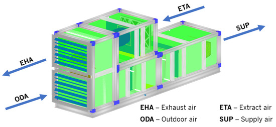
Figure 1.
AHU under analysis and their respective components.
The AHU has two centrifugal fans, one in the supply deck and the other in the exhaust deck. These are dimensioned and selected considering the pressure drop of the components, from each deck, and the installation system pressure drop. Given by the manufacturers, the pressure drops associated with the upper and lower part of the AHU are 549 Pa and 306 Pa, respectively. Along with these, the pressure drop of the supply and exhaust installations are presented. Based on the pressure drop values, the point of operation for each fan was estimated. Table 1 presents the nominal operating conditions of the two centrifugal fans.

Table 1.
Nominal operating conditions of the centrifugal fans.
2.2. On-Site Measurements
In order to obtain data for the numerical simulations and to validate the CFD model, experimental measurements were made on site. It was important to make measurements of the relative pressure in different points of the AHU and the air volume flow rate in circulation. The pressure measurements in the AHU were made, typically, from pressure tips placed in different parts of the machine. The pressure tips located in filters play an important role in the overall maintenance of the AHUs. By measure the filter’s pressure drop, it is possible to estimate their real level of dirtiness. The dirtier the filter is, the higher is the corresponding pressure drop. When a filter is becoming dirty throughout the machine operation, the fan working point changes. Due to the increase of pressure drop, the fan angular velocity also increases to overcome the extra pressure drop. This way, the energy costs due to ventilation increase.
In this way, to measure the values of relative and differential pressure in the different places, a multifunction measuring instrument, the testo 435-4 (accuracy ± 0.02 Pa) was used. This equipment is an air conditioning measurement instrument with a differential pressure gauge integrated. In each measurement test, five measurements were made in order to consider the instrument reproducibility since repeating the measurements, the uncertainty caused by random errors can be determined. Accordingly, to the American Society of Mechanical Engineers guidelines for test uncertainty in instruments, it is recommended that the results are presented with uncertainty for a 95% confidence interval. Therefore, an expanded uncertainty should be calculated through the multiplication of the standard deviation of the mean by an expansion factor (based on a t-student distribution for 95%). More details about the methodology can be found in [13]. In this sense, Table 2 presents the average results complemented with the experimental data uncertainty.
Table 2.
Results of the experiments with an uncertainty for 95% confidence interval.
Measurements at the fan outlet were not possible. However, being the distance between the supply fan and the bag filter entry about 434 mm, it is reasonable to approximate the pressure at the fan outlet to the bag filter inlet pressure. Thus, to compare with the fan technical data from the AHU in the study, the static pressure difference between the fan inlet and the bag filter inlet is considered as the fan static pressure increase. Furthermore, based on these measurements, the air flow rate can be estimated by Equation (1):
where Δp, is the differential pressure, Q is the air volume flow rate worked by the fan and k is a factor that considers the specific properties of the inlet ring of the corresponding fan. Depending on the fan reference, the manufacturers assign different k values for each turbomachine. Thus, the instant air volume flow rate supplied by the fan can be calculated. In Table 3, the fan operating conditions from the AHU from the on-site measurements are presented.
Table 3.
Real operating conditions of the supply fan.
It is possible to verify that, the supply fan is not working under project conditions. There are some reasons that can explain this, as changes in the air flow demand, differences between the project installation layout and the installed layout, or differences between the filters pressure drop during the AHU selection and their real pressure drop in the measurements. In this way, as the fan is working further from its nominal working point, the static efficiency is lower when compared with project conditions. Table 3. shows the operating conditions of the supply fan.
3. Numerical Model
3.1. Mathematical Model and Fan Modeling
The air flow inside the AHU was assumed to be incompressible and turbulent. Although the flow is steady, due to numerical convergence issues the unsteady solution was performed. The unsteady Reynolds-averaged Navier-Stokes governing equations, averaged in a time interval together with the transient term, are applied in the numerical calculation performed by the CFD software (ANSYS Fluent v16.2). Since the flow through the filters passes through a porous media, a source term represented by the term S is added to the momentum equation. Regarding the turbulent field, the realizable k-ε and RNG (Re-Normalization Group) model were considered as both of the models have shown satisfactory results when it comes to flows that include strong streamline curvatures, vortices, and rotation [14]. By doing a preliminary CFD simulation with these two models and comparing their results with the experimental data, it is concluded that the realizable model allows to achieve better results under the conditions of the study. Furthermore, the full buoyancy effects option is enabled to account for the air dynamic of going from lower pressure zones to higher pressure zones. Therefore, the realizable k-ε with a standard wall function is selected because this model is capable to take into account the effects of mean rotation in the turbulent viscosity [14]. The description of these models is presented in detail in the ANSYS Fluent User’s guide [14].
The governing equations were discretized using the Finite Volume Method using a second-order upwind spatial discretization. The computational models were solved using a transient formulation, as in terms of prediction of turbulent flows and swirl phenomena allow better results than steady-state simulations, based on a first-order implicit method and the convergence criterion of 1 × 10⁻³ for continuity and 1× 10⁻⁴ for energy, momentum, and turbulence equations. The pressure-velocity coupling is solved with the Semi-Implicit Method for Pressure Linked Equations (SIMPLE) algorithm, using the standard initialization. The SIMPLE algorithm provides more efficient and robust single-phase flows. The pressure is modeled with a pressure staggering option (PRESTO scheme). The contribution of the gravity acceleration was implemented in a downwards direction.
The simulation of this project was computed in the 12-core processor, with approximately 32 GB of memory RAM required. The simulation time condition was considered unsteady to predict all the movement of gas inside the AHU and the bag filter. The time step size was automatically calculated by the solver upon the previous time step calculation. This algorithm considers the value of the Courant number for the fluid, deciding the next time step size for the simulation.
Subsequently, the results are time-averaged after the simulation reaches a pseudo steady-state by means of a long transient simulation. In all cases, 6 s were enough for the simulation time as after this time the results are stable, varying less than 1%.
Regarding the air flow inside the AHU process where the air is induced by a fan, CFD application, generally, takes one of three approaches to model the turbomachine: Fan Boundary Conditions (FBC) [12], the Moving Reference Frame (MRF) model [2,5], and the Sliding Mesh model [4]. The FBC model is also referred to as the body force model (BFM) in investigation works.
The FBC model is used to determine the fan impact, with certain characteristics, in a flow field. In this case, the fan geometry is not considered, instead, the operating fan curve is introduced in the software. This empirical curve represents the relationship between the fan static pressure rise and the air velocity at the fan inlet, under certain operating conditions. Concerning the second approach, the MRF model, these are steady-state approximations used in problems involving moving parts, such as rotating blades, impellers, and other types of moving parts. Unlike the FBC, MRF models take into account the geometry of the rotating or moving part under analysis. Finally, instead of all the previously presented models, the Sliding Mesh model is an unsteady approach where the transient interactions between the stationary and moving components are accounted for. When modeling turbomachines components, where the interaction between rotor and stator is important, this approach must be used to compute the unsteady flow field. Being the most accurate model for simulating flows in multiple moving reference frames, this is also the one that requires the most computational effort [14].
In this work, the FBC model is used to simulate the air induced by the fan inside the AHU. As mentioned previously, one of the key inputs in this approach is the fan curve equation. To obtain the fan curve equation the similarity between fans is used. The fan manufacturer provides the datasheet from the fan, including several working points at different angular velocities. Using the provided nominal data of the fan, a tendency curve at the real operating conditions is generated. In this way, the real fan working curve, based on the experimental measurements, is presented in Figure 2. It shows the pressure increase as function of the inlet velocity at real operating conditions.
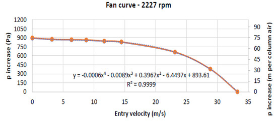
Figure 2.
Pressure increase as function of the inlet velocity at real operating conditions.
As represented in Figure 2, the tendency curve obtained is a fourth-degree polynomial, being the correlation coefficient near unity. Therefore, this curve is used in fan modeling. ANSYS Fluent software calculates the entry velocity at the fan zone, being this value used as an input in the polynomial equation. The pressure increase value is then obtained, and the static pressure values of the adjacent elements to the fan surface are calculated. In this case, a single pressure increase value is determined for the adjacent elements because the option calculates pressure-jump from average conditions is enable [14]. The mass-averaged velocity normal to the fan is determined, and the single pressure-jump value is estimated [14].
The other required inputs for the application of the FBC model were the tangential and radial velocity which were considered as 29.5 and 10.1 m/s, respectively. It is important to note that to reach the values of tangential and radial velocity a real blade angle had to be considered. In this case, a real blade angle of 25° was considered.
The bigger disadvantage of this fan modeling approach is the fact that air flow at the fan outlet is purely radial and tangential. It gains even more important as the exit blade angle of the fan is bigger. Using the FBC model, it is not considering the axial velocity component at the fan outlet. Thus, in the CFD simulations that are presented in the next sections, all the conclusions taken presuppose this limitation.
3.2. Computational Domain, Mesh and Boundary Conditions
The AHU module in the study is only the supply deck (upper part of Figure 1) and it can be divided into four sections: fan inlet, fan outlet, bag filter, and AHU exit. The fan inlet section is defined according to the real distance between the water heating coil, the upstream component of the fan, and the fan inlet zone. The other sections respect the real dimensions of the AHU module, being the AHU exit the zone between the bag filter outlet and the installation conducts. Between the fan inlet and the fan outlet sections is the supply fan, which modeling strategy and considerations are mentioned in the previous section. Furthermore, it is important to note that the considered geometry is defined according to the type of mesh pretended for this case. To improve the stability of the overall simulation process, a structured mesh it is adopted. In this way, in terms of casing constitution, the protrusions from the rails, rivets, and other components are not considered. Thus, each surface respective to all sections is totally flat, being compared to empty sheet metal boxes. The pressure tips, at the top of the fan and bag filter sections, are also not considered. Regarding the fan modeling, this is modeled as a simple disk. This comes because of the fan modeling approach used, where the real geometry of the fan is not needed. Thus, the diameter of the disk is equal to the real impeller diameter, as well as its depth. Furthermore, the fan volute, which is of conic nature, is modeled as a cylinder due to mesh issues. Finally, the fan electric motor is not considered or modeled due to its minor influence on the flow pattern.
Moving into the bag filter modeling, this is assumed as a regular box where geometric details are not modeled. This simplification is possible due to the ability of ANSYS Fluent software of defining a pressure drop in a body, over a certain direction, in the function of its length. Taking into account these considerations, Figure 3a presents the geometry considered for the CFD simulations with the indication of the boundary conditions. The yellow line presented in Figure 3a, which crosses the whole system, is represented since a curve of the static pressure evolution over the system length will be carried out to better interpretation and comparison of the different CFD results. Figure 3b shows the mesh used in the study.
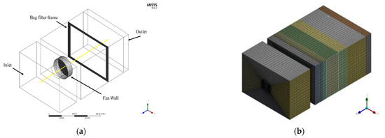
Figure 3.
Representation of the: (a) AHU geometry and (b) mesh used in the simulation.
The strategies assumed in the geometric modeling are based on the need of building a structured mesh. In this sense, to better control the structured mesh features, some splits over the geometric model were performed. An isometric perspective of the mesh obtained is presented in Figure 3b). Mesh refinements were performed in specific zones where there are high gradients of velocity or pressure. Thus, higher mesh resolutions in the regions with higher gradients allow defining better transition zones. In terms of mesh quality evaluation, there are some crucial mesh parameters commonly used in the literature, as orthogonality, skewness, and aspect ratio. These parameters were evaluated, and it was possible to conclude that the mesh is in lined with all the main quality parameters regularly used in the literature. After this analysis, a mesh dependency study was carried out. This study allows for the assessment of the dependency of the CFD results in the mesh resolution (number of elements), without changing the mesh quality standards. Four different meshes were developed and preliminary simulations were done and at the end of the simulation, the air flow rate was computed. Figure 4 presents the results, and it is possible to see that the maximum difference between the air flow rate is less than 1%. Furthermore, the air flow rate stabilizes, approximately, at 3971 m3/h and, therefore, to reduce the computation time and effort, only 560,784 hexahedral elements are necessary.
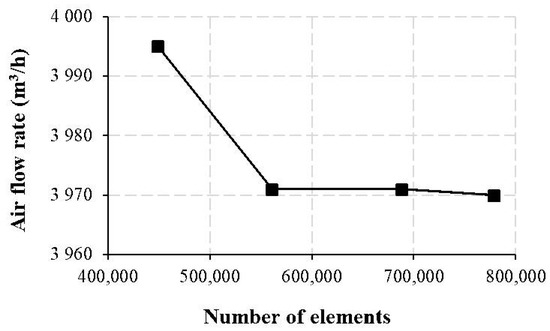
Figure 4.
Mesh dependency study.
Another important aspect concerning the mesh resolution, the y + value was considered during the mesh execution. In this regard, the fact that the flow pattern in the analysis is dominated by swirl, the need for high resolution meshes is lower and this was taken into account. Consequently, the turbulence stresses are dominant relative to the Reynolds shear stresses (the y + can be higher than 30 to capture the fully turbulent layer which is where turbulent stress dominates the flow). Thus, with the mesh resolution considered, the values of wall y+ are higher than 30 in all wall zones, and, consequently, a standard wall function was used to accurately predict the flow in the boundary layer.
In terms of boundary conditions, its values were defined considering the experimental measurements (Table 4).
Table 4.
Boundary conditions defined in the numerical model.
A pressure inlet and outlet were defined at the inlet and outlet, respectively. Table 4 also presents the condition defined for the fan and bag filter wall.
Furthermore, the bag filter region was modeled as a box, by defining a pressure drop in the function of its length, in the direction of the air flow (z direction). Considering the pressure drop obtained on-site measurements, a source term in the Z Momentum equation is defined as 413.2 N/m3.
4. Results and Discussion
4.1. Validation of the Numerical Model to Nominal Operating Conditions
To analyze the accuracy of the FBC model, the CFD simulation was developed from the data provided by the on-site measurements. By defining a longitudinal plane, xz plane, located at medium height, it is possible to observe the static pressure and velocity contours, as represented in Figure 5 and Figure 6, respectively.
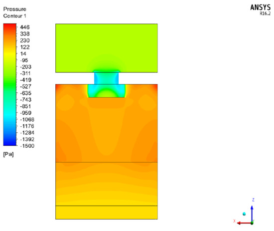
Figure 5.
Static pressure contour at medium height of the AHU.
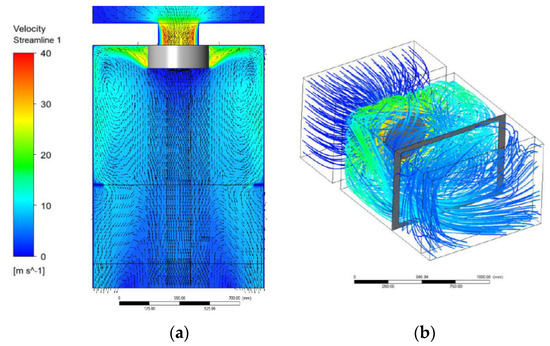
Figure 6.
Velocity field inside the AHU: (a) velocity contour and velocity vectors at medium height and (b) velocity streamlines inside the AHU.
The static pressure in the fan volute reaches very low values. In this zone, the dynamic pressure component is also important due to the high passing air velocity. In terms of static pressure field calculated, it is seen, as mentioned previously, that an average value of static pressure is set in the fan zone boundary.
Furthermore, it is understood that the fact that the air flow at the outlet is purely radial and tangential, makes that the zones with higher static pressures are located at the near-wall zones. This phenomenon creates “death zones” where the static pressure levels are lower, and around where swirl formation takes place. Finally, the pressure drops defined for the bag filter over z direction, in the function of its length, can also be observed in Figure 5.
Figure 6 shows the velocity field inside the AHU: (a) velocity contour and velocity vectors at medium height and (b) velocity streamlines inside the AHU.
Regarding the velocity contour (Figure 6a), a maximum velocity of approximately 40 m/s was found. This velocity is reached in the fan volute, where there is a shrinkage of the air flow, as expected. The air flow at the fan outlet is purely radial and tangential, being in the near-wall zone where the air flow evolves. It is possible to verify that in the middle of the domain, the velocity is lower. If the fan real geometry was taking into account, due to the exit angle of the fan blades, the air velocity at the fan outlet would have an axial component.
The velocity streamlines presented in Figure 6b show the high level of turbulence of the air flow in the study. The visible zones in grey are the fan wall and the bag filter frame.
The big issue in this study case is the swirl generated by the high levels of turbulence. By projecting the velocity vectors, tangentially, into a xz plane located in medium height, is possible to see the formation of a swirl. The swirl is a mechanism of energy dissipation, and, thus, a pressure drop source. This phenomenon is important and may have a big impact on the performance and energy consumption of the AHU.
To check the precision and applicability of the FBC model, the fan pressure increases and the air volume flow rate, are analyzed. As mentioned before, the considered fan static pressure increase is the difference between the pressure measured in the fan inlet and in the bag filter inlet. This is the differential pressure that is used to compare the experimental and CFD results. Table 5 presents an overview of the experimental and numerical results and its difference.
Table 5.
Experimental and numerical results.
There are several conclusions that can be taken from Table 5 results. First, all the measurements were done by a five repetitions process per variable. Being the AHU in operation at the time of the experimental measurements, the values can vary considerably due to several uncontrolled factors. The air volume low rate error may be due to two different reasons. Initially, the fact that the static pressure considered at the inlet zone is the one measured at the fan inlet. Second, the experimental value for the air flow rate is not a measured value but an estimated value. As presented in Section 2.2, the air volume flow rate is achieved from the fan differential pressure measured on-site, and the corresponding fan k factor. Beyond the uncertainties in the experimental measurements, the manufacturer approach to achieve the air flow rate worked by the fan has associated an error of 5 to 6%. Finally, uncertainties associated with the geometry simplifications done and the FBC model utilization have an impact on the air flow rate calculation.
When it comes to the fan differential pressure results, it is seen that the error obtained is 42.2%. There are some explanations for this, as the simplifications in terms of the fan volute geometry and the fan modeling approach used. Then, the installation method of the pressure tips inside the AHU becomes a problem. In this case, the pressure tips have, approximately, 50 mm in length. This allows the formation of micro-swirl phenomena around the tubes, adulterating the pressure values read. This problem does not affect only this parameter but all the others. Another cause for the error obtained is in the flow pattern at the inlet section. In the CFD simulation, the air flow at the inlet section is relatively stable and does not have any rotational component associated. In fact, the flow is relatively turbulent and highly rotational.
Another important parameter in the analysis is the fan pressure increase. As seen in Table 5, an error of 21.5% is obtained for this parameter. It is relatively high, but there are some issues. The FBC model is very dependent on the quality of the fan curve used as input. In this case, using some tested working points given by the fan manufacturer a fan curve at nominal conditions is obtained. Although, in the fan datasheet, only four to six working points are given for nominal conditions. This leads to a fan curve that is not very reliable. Furthermore, to achieve the fan curve at real working conditions the similarity between fans approach is used, which is an approximation. All these factors combined have an impact on the results.
Looking at the results in the bag filter, the errors found in pressure are associated with the model used in the CFD simulations. As previously mentioned, for the bag filter modeling, using the on-site measurements, it is defined as a pressure drop in the function of its length (z direction). Thus, the pressure drops induced by the bag filter, in ANSYS Fluent software, is only in the Z direction. It does not happen in a real AHU, where the pressure drop in a bag filter acts in every direction. Still, due to the high level of turbulence of the air flow in circulation, this problem gains more meaningfulness.
Despite all the limitations of the FBC model, this model is validated and chosen to accomplish the CFD simulations that are presented in the next sub-sections. Its simple application, its low requirements in terms of computational effort, and hardware make this model very attractive.
4.2. Improvement of the Air Handling Unit Performance
After the evaluation of the applicability of the FBC model to model the air flow inside an AHU, the potential of the rectangular cuboid-shaped body downstream of the fan is evaluated. The installation of a cuboid-shaped body at the exit zone of the centrifugal proved to be an interesting option to decrease the turbulence levels downstream of the centrifugal fan [12]. With this solution, most of the conduct area is covered, leaving only a small channel for the air at the near zone of the conduct walls to pass. The use of this body allows to increase the fan efficiency by reducing the vorticity downstream of the fan, transferring a substantial part of the kinetic energy into pressure energy (static pressure).
To this body, for this investigation, the name of Flow Control Unit (FCU) is given. Two different sizes of FCU are studied. The dimensions are 527 mm × 760 mm × 250 mm and 592 mm × 879 mm × 250 mm for FCU 1 and FCU 2, respectively. The mesh and boundary conditions used for these simulations are the same presented before.
Figure 7 shows the pressure contour inside the AHU with (a) FCU1 and (b) FCU 2. Represented as a grey box, in Figure 7, the effect of the FCU 1 and FCU 2 can be observed. A general increase of static pressure in the near-wall zones was obtained due to the utilization of an FCU. When comparing FCU 1 and 2, the static pressure levels with FCU 2 are higher.

Figure 7.
Pressure contour inside the AHU with (a) FCU1 and (b) FCU 2.
Regarding the velocity field inside the AHU, the FCU acts as a minimizer of the swirl generated in the near-wall zones and even lower with FCU 2. Figure 8 shows the velocity contour inside the AHU with (a) FCU1 and (b) FCU 2 it is clearly seen that the FCU reduces the vorticity downstream of the fan, by comparing it with the velocity vectors obtained in Figure 6. The shrinkage between the FCU wall and the AHU wall provokes an increment in the air velocity, minimizing thus the swirl formation. By decreasing the air flow area of passage, the air velocity variation in the perpendicular direction of the AHU wall, x direction, in this case, is increased. Therefore, the shear stress in the shrinkages increase. Despite the fact that the pressure drops increases in these zones, the decreasing of dissipated energy due to swirl formation is the most significant.
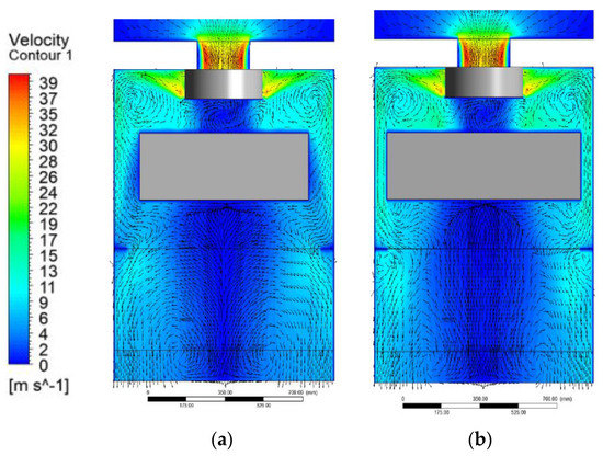
Figure 8.
Velocity contour inside the AHU with (a) FCU1 and (b) FCU 2.
Figure 9 shows the static pressure curves obtained with and without FCU, under real conditions. At the fan exit, the static pressure obtained with FCU 2 is lower than the obtained without FCU, as in the case with FCU 1. This may be justified by the transformation of a part of the air flow energy into kinetic energy due to the shrinkages induced by FCU and, consequently, a decrease of the pressure energy (static pressure). In the transition between the fan outlet and the beginning of the FCU 2, there is an increase of the static pressure before stabilizing through the FCU 2. The reason behind it may be the decreasing of the kinetic energy due to the shocks of the air flow against the FCU 2. Being the cross-section area of the FCU 2 higher than FCU 1, these phenomena may start to have an impact and the static pressure rises. After the FCU, there is an air expansion and there are transformations of kinetic energy into pressure energy.
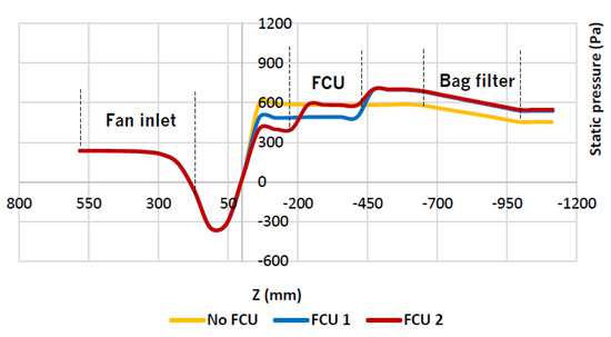
Figure 9.
Static pressure curves obtained with and without FCU, under real conditions.
The inclusion of a FCU resulted in a static pressure rise improvement of 15.1% and 19.2% with FCU 1 and FCU 2, respectively.
However, the results obtained with FCU 2 can be misleading in terms of the possible real losses due to air flow shocks against the FCU 2 front wall.
The previous investigation allowed to ensure that the FCU has huge potential to produce a useful effect in the flow pattern downstream of a centrifugal fan. However, further improvement can be achieved by a geometry optimization of the FCU 1.
The influence of changing the downstream geometry of FCU 1 in the fan static pressure increase appears to be an interesting option to reduce the static pressure. Figure 10 shows the new design of the FCU inside the AHU: (a) view in perspective and (b) side view (right). As seen in Figure 10, the modified geometry has conic features in its downstream part. This shape is similar to a common conduct transformation used to connect a rectangular section to a circular section. For this case, it is given the name of FCU Alpha to the FCU with modified geometry. The performance of FCU 1 and FCU Alpha is compared by assuming that their front section area (rectangular) and total depth are equal. In the case of FCU Alpha, the rectangular part has 100 mm depth, and the conic part has 150 mm depth.
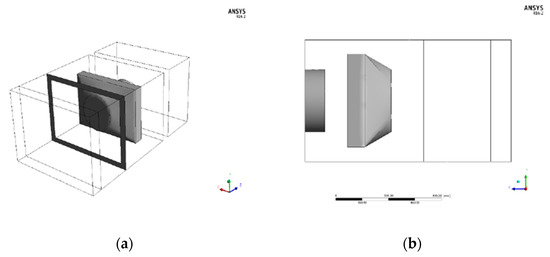
Figure 10.
New design of the FCU inside the AHU: (a) view in perspective and (b) side view (right).
The air flow pattern with FCU Alpha is presented in detail, with the contour at medium height and streamlines in Figure 11. The velocity field inside the AHU with the FCU optimized is represented: (a) velocity contour and velocity 370 vectors at medium heigh and (b) velocity streamlines inside the AHU. Looking at the velocity vectors obtained with FCU Alpha (Figure 10a), differences downstream are found when compared with the results obtained with FCU 1 (Figure 6a). With FCU Alpha, the air flow develops more in the middle of the AHU, as can be observed at the bag filter zone. Although, no additional relevant differences are seen in terms of air flow patterns.
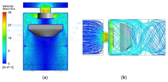
Figure 11.
Velocity field inside the AHU with the FCU optimized: (a) velocity contour and velocity vectors at medium height and (b) velocity streamlines inside the AHU.
Apart from the velocity analysis, Figure 12 shows the static pressure curves obtained with FCU 1 and FCU Alpha, under real conditions.
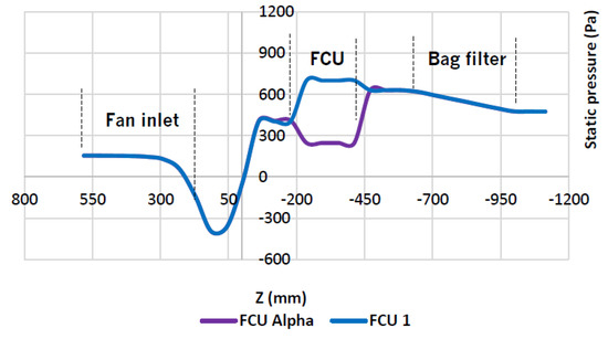
Figure 12.
Static pressure curves obtained with FCU 1 and FCU Alpha, under real conditions.
Static pressure curves obtained with FCU 1 and FCU Alpha over the whole domain are presented. An improvement in static pressure rise of 6.1% with FCU Alpha relative to FCU 1 is obtained. The reason why this value is relatively low may be due to the small distance between the fan exit and the bag filter entry. The objectives with FCU Alpha and its downstream geometric features were to improve the stability of the air flow at the bag filter inlet and decrease the Reynolds shear stress at the boundaries and downstream of the FCU. By transforming a bigger part of the energy, when passing around the FCU Alpha, in pressure energy, the objective was to achieve a higher value of static pressure rise relative to FCU 1.
Despite the improvement in the static pressure rise with FCU Alpha, it is was not expected a lower outlet static pressure. Being static pressure improvement relatively low, this difference may be due to mesh problems.
5. Conclusions
The present work focuses on the analysis of the fluid flow inside an AHU. From this perspective, a numerical model, using the ANSYS Fluent software, was developed to investigate and understand the fluid flow inside this type of machine and to study alternative constructive solutions in order to optimize the operation of the AHU. In this research work, the most important findings are summarized as follows:
Results of industry-academic collaboration to apply scientific research to understand and improve industrial products can be used to deliver more efficient products. In this case, a new design philosophy was explored with promising results that need more extensive development to optimize the concept.
The results obtained with the FBC model, when compared to the experimental measurements, are quite different. The considered fan modeling approach has revealed a decent agreement with the experimental results in terms of air volume flow rate calculated, despite the simplifications and assumptions are taken. Although, for the other parameters, as fan static pressure rise and bag filter pressure drop, relatively high errors were obtained. Several are the possible causes for these errors, as the geometric simplifications adopted, errors in the experimental measurements, and simplifications in terms of CFD inputs. Despite that, the FBC model has proved to be simple to use and light in terms of computational effort, making it attractive to be applied.
Moving into the FCU 1 and FCU 2 investigation, the results allowed to conclude that, considering the modeling approach, the static pressure rise improvements can be obtained, although the difference between both FCUs is minimum.
There should be an optimum FCU size, for certain working conditions and AHU casing, where the profits of the usage of an FCU overlap the pressure losses due to the impact of the air flow against the FCU front wall. Although, it is noticed the capacity and potential of the FCU in decreasing the recirculation phenomena downstream of a centrifugal fan, an approach considering the real geometry of the fan blades is required, despite of its expensive costs.
When it comes to the FCU optimization study, an improvement in static pressure rise of 6.1% is obtained. Additionally, other important aspects need further investigation. An example of that is the depth of the conic part of FCU Alpha. In a bigger AHU, where the depth of FCU Alpha could be higher, a higher stabilization of the air flow is expected, and, thus, higher improvements in static pressure rise. Furthermore, the angle formed in the transition between the rectangular and conic parts of FCU Alpha could also be very important.
With all these investigations, it is seen that there is considerable potential in the mounting of an object at the exit of a centrifugal fan. Being known that, nowadays, most of the AHUs incorporate EC Plug fans, a decrease in the specific fan power of AHUs is expected with solutions like the FCU. For a certain working point of an EC Plug fan, a decreasing of its angular velocity is expected with the mounting of an FCU due to the decreasing of the pressure drop at the fan exit. Although, experimental tests need to take place to clearly see the reaction of the centrifugal fan to the mounting of an FCU.
Author Contributions
Conceptualization, J.L.; J.S.; J.T.; methodology, J.L.; J.S.; J.T.; investigation, J.L.; J.S.; writing—original draft preparation, J.L.; J.S.; J.T.; S.T.; writing—review and editing, J.L.; J.S.; J.T.; S.T.; supervision, J.T.; S.T. All authors have read and agreed to the published version of the manuscript.
Funding
This work was supported by Portuguese Foundation for Science and Technology (FCT) within the R&D Units Project Scope UIDB/00319/2020 (ALGORITMI) and R&D Units Project Scope UIDP/04077/2020 (MEtRICs).
Acknowledgments
The second author would like to express his gratitude for the support given by FCT through the Grant SFRH/BD/130588/2017.
Conflicts of Interest
The authors declare no conflict of interest.
Nomenclature
| k | factor for each turbomachine, - |
| p | pressure, Pa |
| Q | Air flow rate, m3/s |
References
- Shahsavar Goldanlou, A.; Kalbasi, R.; Afrand, M. Energy usage reduction in an air handling unit by incorporating two heat recovery units. J. Build. Eng. 2020, 32, 101545. [Google Scholar] [CrossRef]
- Chunxi, L.; Ling, W.S.; Yakui, J. The performance of a centrifugal fan with enlarged impeller. Energy Convers. Manag. 2011, 52, 2902–2910. [Google Scholar] [CrossRef]
- Rong, R.; Cui, K.; Li, Z.; Wu, Z. Numerical Study of Centrifugal Fan with Slots in Blade Surface. Procedia Eng. 2015, 126, 588–591. [Google Scholar] [CrossRef][Green Version]
- Vasudeva Karanth, N.M.K.; Yagnesh Sharma, N. Effect of innovative circular shroud fences on a centrifugal fan for augmented performance—A numerical analysis. J. Mech. Sci. Technol. 2018, 32, 185–197. [Google Scholar]
- Shen, Y.; Li, Y.; Wang, H.; Shen, W.; Chen, Y.; Si, H. Numerical simulation and performance optimization of the centrifugal fan in a vacuum cleaner. Mod. Phys. Lett. B 2019, 33, 1950440. [Google Scholar] [CrossRef]
- Bleier, F.P. Fan Handbook: Selection, Application, and Design; McGraw Hill Higher Education: New York, NY, USA, 1998. [Google Scholar]
- Bozkaya, B.; Zeiler, W. The energy efficient use of an air handling unit for balancing an aquifer thermal energy storage system. Renew. Energy 2020, 146, 1932–1942. [Google Scholar] [CrossRef]
- Yun, G.Y. Influences of perceived control on thermal comfort and energy use in buildings. Energy Build. 2018, 158, 822–830. [Google Scholar] [CrossRef]
- Schito, E. Dynamic simulation of an air handling unit and validation through monitoring data. Energy Procedia 2018, 148, 1206–1213. [Google Scholar] [CrossRef]
- Nilsson, L.J. Air-handling energy efficiency and design practices. Energy Build. 1995, 22, 1–13. [Google Scholar] [CrossRef]
- Li, S.; Wen, J. Development and Validation of a Dynamic Air Handling Unit Model, Part I; ASHRAE Transactions United States of America: Atlanta, GA, USA, 2010; Volume 116. [Google Scholar]
- Azem, A.; Mathis, P.; Stute, F.; Hoffmann, M.; Müller, D.; Hetzel, G. Efficiency increase of free running centrifugal fans through a pressure regain unit used in an air handling unit. Energy Build. 2018, 165, 321–327. [Google Scholar] [CrossRef]
- ASME. Test Uncertainty PTC 19.1—2018(R2018); ASME: New York, NY, USA, 1998. [Google Scholar]
- ANSYS. ANSYS FLUENT Theory Guide; ANSYS: Canonsburg, PA, USA, 2013. [Google Scholar]
Publisher’s Note: MDPI stays neutral with regard to jurisdictional claims in published maps and institutional affiliations. |
© 2020 by the authors. Licensee MDPI, Basel, Switzerland. This article is an open access article distributed under the terms and conditions of the Creative Commons Attribution (CC BY) license (http://creativecommons.org/licenses/by/4.0/).