Off-Design Exergy Analysis of Convective Drying Using a Two-Phase Multispecies Model

Abstract

The design of a convective drying cycle could be challenging because its thermodynamic performance depends on a wide range of operating parameters. Further, the initial product properties and environmental conditions fluctuate during the production, affecting the final product quality, environmental impact, and energy usage. An off-design analysis distinguishes the effects of different parameters defining the setup with the best and more stable performance. This study analyzes a reference scenario configured as an existing system and three system upgrades to recover the supplied energy and avoid heat and air dumping in the atmosphere. We calculate their performance for different seasons, initial product moisture, input/output rate, and two products. The analysis comprises 16 simulation cases, the solutions of a two-phase multispecies Euler–Euler model that simulates the thermodynamic equilibrium in all components. Results discuss the combination of parameters that maximizes the evaporation rate and produces the highest benefits on global performance up to doubling the reference levels. The advantages of heat recovery vary by the amount of wasted energy, increasing the exergy efficiency by a maximum of 17%. Energy needs for air recirculation cut the performance at least by 50%. Concluding remarks present the technical guidelines to reduce energy use and optimize production.

1. Introduction

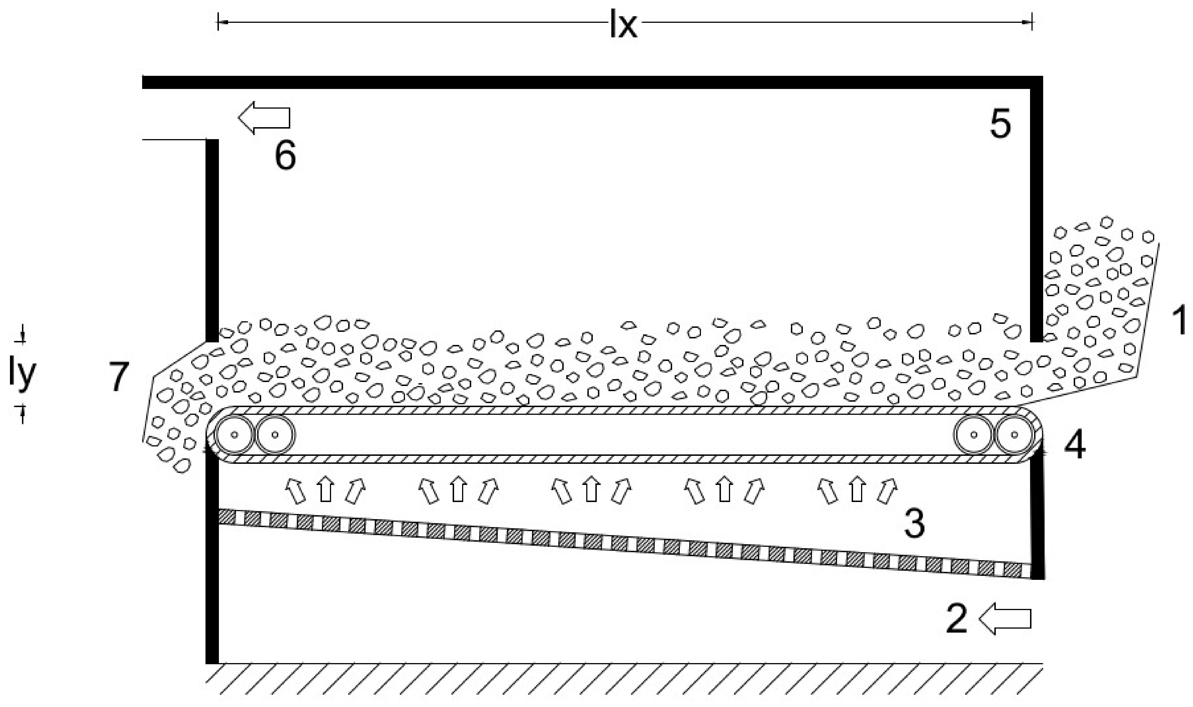
Thermal drying plays a crucial role in several industries, such as chemical, pharmaceutical, agricultural, and food production. It involves heating a wet product to evaporate its liquid fraction and generating a thermally induced mass flux [1]. According to the dominant energy transfer mechanism, thermal drying can be categorized into convective [2], conductive [3], and radiative drying [4]. The present study focuses on convective drying operated as a continuous process on a horizontal fluidized bed (Figure 1).

The fluidized bed systems present several advantages as a good mixing quality (homogeneous temperature distribution along the bed) and high heat and mass transfer rate caused by the extended contact surface between the solid particles, and the gaseous phase [5,6]. However, reaching the optimal thermodynamic performance of such systems needs careful tuning of numerous operating parameters that influence the final energy consumption, product quality, and environmental effects.

For example, the finest particles (powder) tend to agglomerate, affecting the evaporation rate and quality of the final product [7]. This effect increases the bed pressure drop; thus, a faster airflow becomes necessary to preserve product quality, but it increases the final energy consumption, and costs [8]. Further limitations of the global performance derive from the unavoidable inefficiencies of the process: the sensible heating of the dry fraction, the heat losses of the drying chamber, and the low thermal conductivity of the heat transfer media (air), which demands high operative temperatures to drive adequate heat flux [9]. Another issue regards the effect of the environmental conditions on the final energy use: the analysis of Reference [10] reveal the drying chamber as particularly susceptible to the external temperature; its performance deteriorate with temperature fluctuations of approx. 5 ${}^{\circ }$C. Finally, some specific applications such as the convective drying of biomass and hazardous materials, release several pollutants into the atmosphere; this deteriorates local air quality and contributes to greenhouses gas emissions [11,12,13]. For such reasons, stringent environmental regulations limit their functioning.

In the design and optimization practice, predicting all the effects mentioned above can be challenging because of the relations among the drying parameters and the mutual dependencies among the system components [14]. The standard approach studies the relation between the drying conditions and final performance by the energy analysis of the drying chamber. Dincer et al. [15] calculated the efficiency of the cycle (i.e., drying efficiency) as the ratio between the energy invested in the evaporation process over the total energy entering the drying chamber by hot airflow. Further studies [16] included the specific energy consumption, calculated as the amount of consumed energy per unit mass of the evaporated moisture.

Energy analysis by itself cannot calculate the operative costs and any form of environmental effect because it does not distinguish the primary energy source; such an approach does not provide any information regarding the effects of the climate on system productivity. To overcome these limitations, several authors included the exergy analysis in the evaluation of system performances.

The first exergy analysis of convective drying is presented in Reference [17], wherein the authors calculate the exergy efficiency of the drying chamber as the ratio between the exergy invested in the evaporation process to the total exergy of the entering airflow. Assuming the entering product is at a dead-state, the exergy investment is the exergy of the total evaporated moisture leaving the drying chamber. Several works follow the approaches presented above. Akpinar et al. [18] related the energy utilization of the drying chamber with an evaporation rate and initial product moisture; they measured an increase in exergy losses using the drying air temperature and velocity. Yogendrasasidhar et al. [19] analyzed the effect of the several drying parameters on the energy utilization, exergy losses, and exergy efficiency of the system: by increasing the wall temperature and air velocity, the energy usage augments but the exergy losses decreases with benefits on the final exergy efficiency; the prolonging of drying time produces a two-fold benefit by reducing energy usage and exergy losses and by increasing exergy efficiency. Aviara et al. [20] showed a linear dependence between energy efficiency and the drying air temperature.

More recent research on convective drying oriented the exergy analysis toward optimization by comparing different system configurations and operative conditions. Icier et al. [21] compared the exergy performance of two open drying cycles and a closed cycle, where drying air was recovered from the drying chamber and heated by a heat pump. Xiang et al. [22] analyzed a drying system coupled to a heat pump; in particular, they investigated how the system performance changes under different operative conditions, varying the amount of recirculating air (from an open to a fully-closed cycle). Cay et al. [23,24] analyzed and compared two open cycles, in which internal and external combustion chambers heat the drying air, respectively. Erbay [10], and Gungor [25] investigated how dead-state temperature affects the exergy performance of a drying system fed by a ground source and a gas heat pump.

All studies presented above refer to the given system configurations; their results are valid only under the working conditions observed for the analyzed system and can be used for designing the drying cycle of a specific material. Furthermore, limiting the performance analysis to the drying chamber misses the most recent and accurate optimization techniques of energy systems that extend the exergy analysis to a multicomponent level (they calculate the exergy destruction in a single component by considering interdependencies with all other components) [26,27]. Thus, the research gap in the current literature is based on the design approach specifically formulated for convective drying, which considers the effects of changing the system configuration and operative conditions (e.g., dry another product, adding another component, and varying the climate) for the optimization of thermodynamics and costs [28].

The design of a drying system needs a theoretical model to calculate the state of working flows in the different components (i.e., thermodynamic equilibrium model). The Euler–Euler description is a common approach to simulate the thermodynamic equilibrium of a drying process due to its low computational costs and the capability to simulate fluids with a high concentration of the dispersed phase [29,30,31]. Assari et al. [32,33] studied the drying of wheat grain: first, they formulated a two-fluid model to investigate the effects of varying the operative conditions on the main operative parameters of the drying bed (e.g., void percentage and air humidity); in the following study, they analyzed the exergy performance. Li et al. [34] modeled two fluids, the bubbly and emulsion phases, a mixture of an interstitial gas, and a solid phase; using this formulation, they performed a sensitivity analysis of the drying performance with respect to the state of inlet air, particle diameter, and wall temperature of the drying chamber. Ranjbaran et al. [35] developed a two-fluid model for paddy drying; they investigated the temporal variation of the energy and exergy efficiency during the drying process with effects of air temperature and flow rate; a source term in transport equations is used to model the evaporation of moisture. Rosli et al. [36] simulate the drying of sago waste by a two-fluid model of the drying column; they investigate by CFD the effects of different drying conditions (e.g., the air velocity, temperature, and particle size) on the fluidization of the bed. Jang et al. [37] simulate a fluidized bed dryer by an Euler-Euler model coupled to empirical correlations representing the inter-phase exchanges; the authors investigate the advantages of such a model in the design and scaling-up of pharmaceutical applications.

The above studies simulated the drying process by two homogeneous phases—the drying air and the wet solid—without focusing on their chemical composition. A multispecies approach enhances the versatility and accuracy of the two-fluids theory—it comprehends the effects of each species on the mass and energy fluxes [38]. Furthermore, this approach can simulate applications of reactive flows according to the stoichiometry of the ongoing chemical reactions (e.g., combustion of a hydrocarbon for air heating). The multicomponent theory generally finds applications in petroleum distillation [39,40], while the available literature lacks references for applications to convective drying.

In addition to the thermodynamic equilibrium model, the design of a drying system needs characteristic equations describing the heat and mass transfer phenomena that occur in each component; as an example, the characteristic equation of the drying chamber is the evaporation model. Defraeye et al. [41] derive the characteristic equation of drying by a theoretical approach—the authors analyze the convective drying of a porous flat plate by solving the transport phenomena at the interface between the porous media and the airflow, explicitly. Such an approach, known as conjugate modeling, describes in detail the physics of the heat and mass transfer; however, despite its accuracy, just a few academic applications use this technique because of the high complexity, and computational costs [30]. Quite the opposite, the empirical or non-conjugated models derive from experimental observations and describe the heat and mass transfer by constant coefficients, with a limited understanding of the involved physics. Some well-known examples of empirical models are Newton’s law of cooling, and the evaporation model of Page [42].

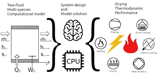
Our study investigates the thermodynamic performance of convective drying under different operating conditions and system configurations; the final aim is distinguishing the parameters with the most significant effects on the energy use and product quality to define the setup with the best performance. We follow a theoretical approach, named off-design analysis applied successfully for the optimization and control strategies of various energy systems [43,44,45]. The novelty of our work is the nature of the studied application: in the literature, there is not any off-design analysis of convective drying; in particular, the current design practice lacks a theoretical formulation for modeling the state of working flows in the drying chamber and all system components, including the devices for heat and mass recovery. The level of detail of our theoretical approach is a further innovation in the field of drying modeling: we formulate the two-fluids theory describing the thermodynamic equilibrium of the single chemical species to simulate all components of the drying system. Finally, due to the adaptability of the solving algorithm, we present an innovative tool for both design new drying cycles and verify the states of working flows in existing systems.

The presented equilibrium model includes the multispecies approach in the two-fluid theory to simulate all the components of a drying system; in particular, we follow a two-fluid multispecies Euler–Euler (TFMM) approach to simulate the following processes.

• Mass and energy exchange between nonreactive phases: Convective drying of a wet solid and air-water counter-current mixing;
• Mass and energy exchange between reactive phases: combustion of airflow by a hydrocarbon jet;
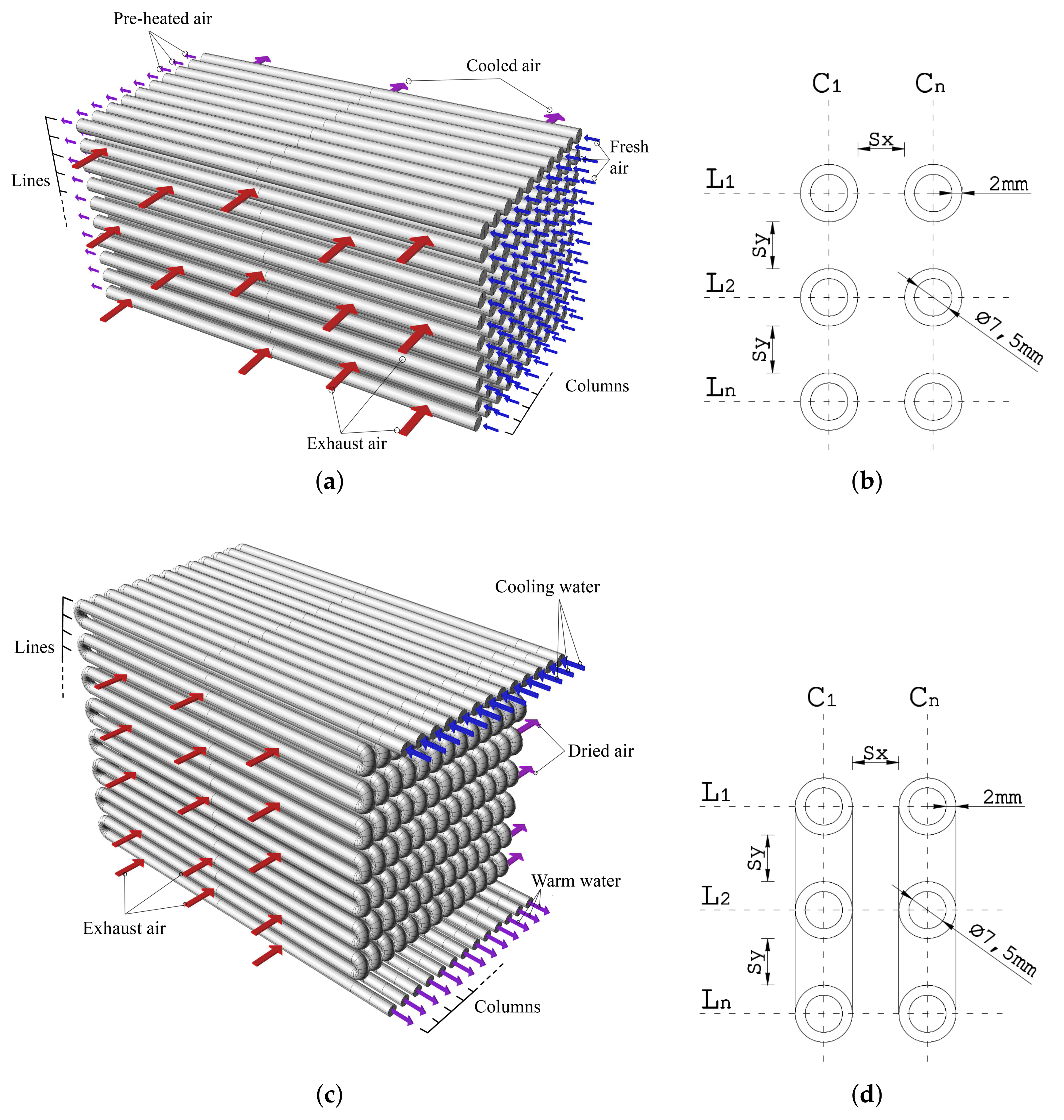
• Energy exchange between nonreactive phases: Air-to-air and air-to-water heat exchange within a tube bank.

Our analysis aims to support the design practice of a drying system rather than investigate drying physics in detail. Thus, we simulate heat and mass exchanges by empirical equations because of their appropriate accuracy for the scale of simulated processes (macro-scale between 0.01–10 m [30]), as well as the advantages of a simple mathematical formulation and low computational costs.

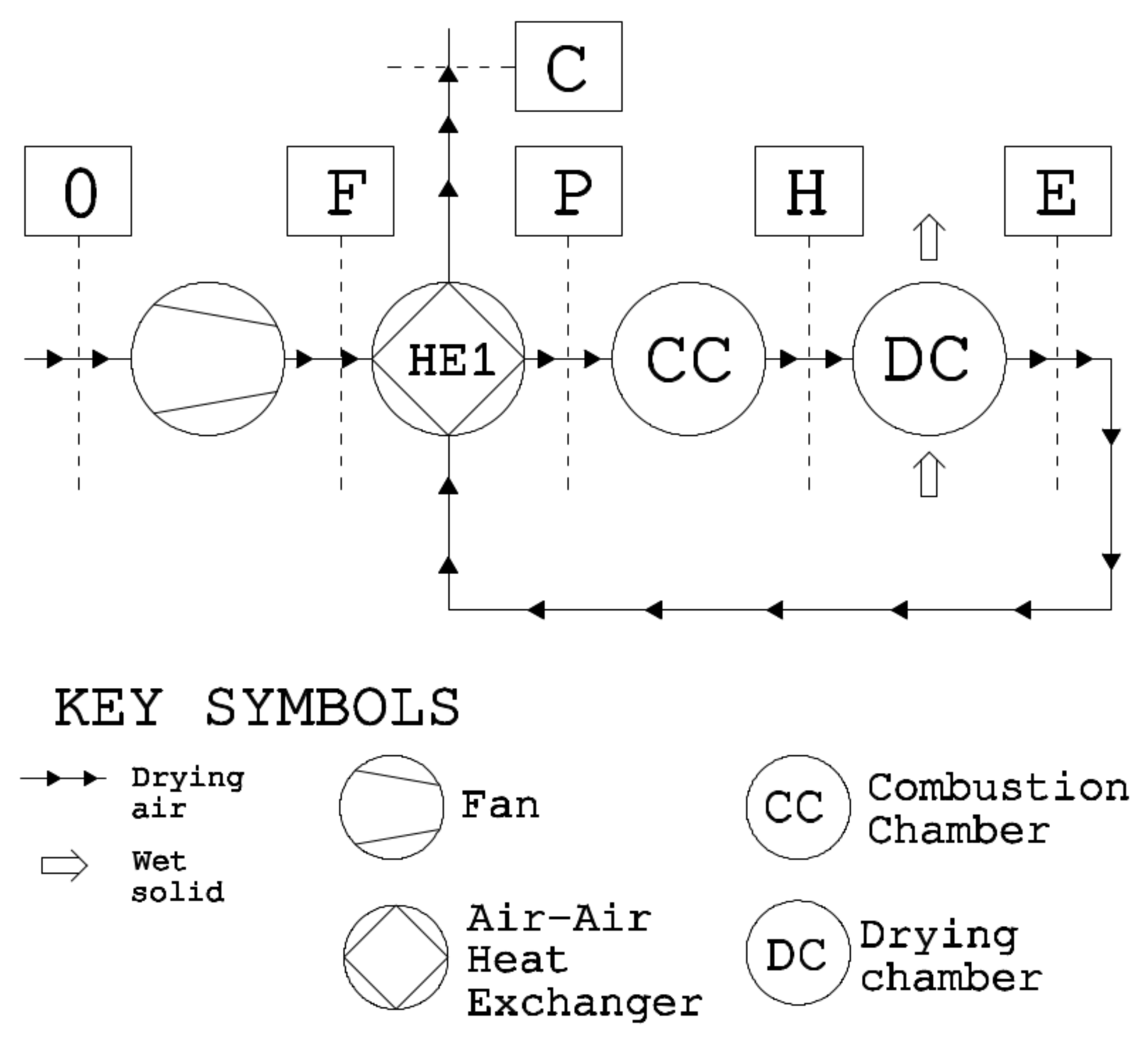
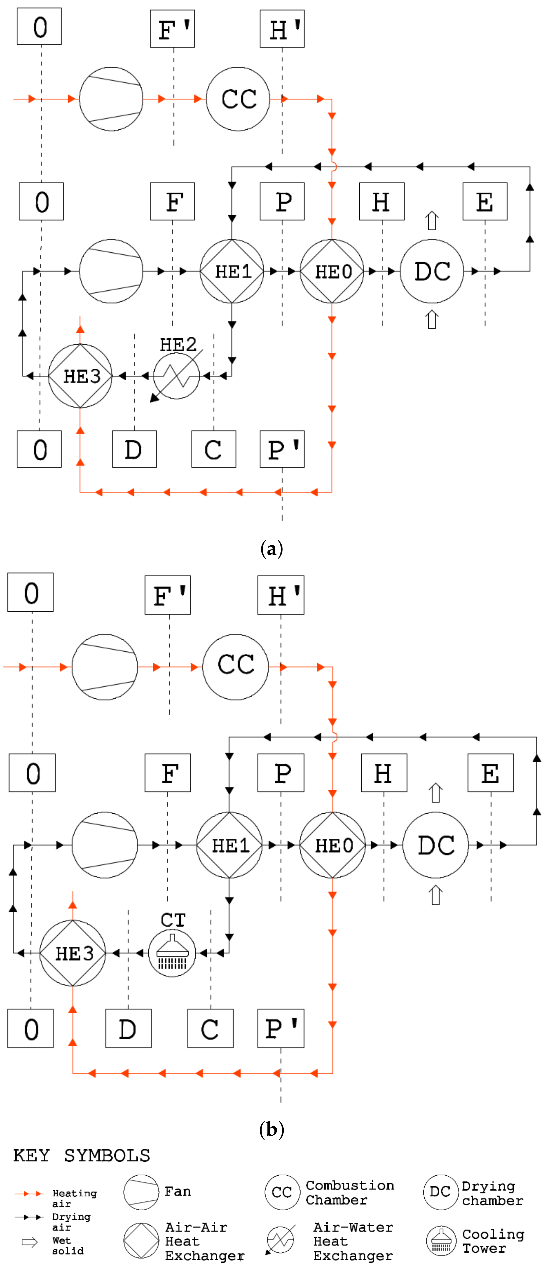
The analysis starts with the exergy analysis of a reference drying cycle, named the baseline scenario, based on an existing industrial system; this scenario mounts the essential components of convective drying: fan, combustion chamber, and drying chamber (Figure 1). We calculate the baseline performance at the operative conditions of the existing system and validate the results against experimental data. Later, we change the drying conditions, dead-state conditions, and dried material to investigate the effects on energy consumption and exergy efficiency. By the last set of operative conditions, we assess the drying of municipal sewage sludge, thereby aiming to contribute to this crucial but scarcely investigated sector. Finally, we modified the reference system to investigate the effects on the global performance of heat and mass recovery by three different layouts.

2. Research and Method

2.1. Governing Equations

We assume that all thermodynamic processes of a convective drying cycle occur in a one-dimensional open system of infinitesimal $dx$ length (Figure 2). To support the assumption of a one-dimensional system, we calculate the heat and mass exchange rates by the lumped-system model (e.g., the Page model for drying and Newton’s cooling law for heat exchangers; see more details in the Appendix A).

The TFMM describes the mass and energy exchanges, entropy generation, and exergy destruction: Phase 1 is drying air, which is a semi-perfect gas mixture; Phase 2 is the substance that exchanges mass and heat with drying air (its state and composition vary by the nature of the simulated process).

Assuming equilibrium between the j-species dispersed in the i-phase, we track them by their respective mass fractions

$${\alpha }_i=\frac{m_i}{m_{os}}$$

(1)

$${ϵ}_{ij}=\frac{m_{ij}}{m_i}$$

(2)

where

$$m_{os}=\sum _i{m}_i$$

(3)

$$\sum _i{\alpha }_i=\sum _j{ϵ}_{ij}=1.$$

(4)

• Mass balance of j-species per unit length is

  $$\frac{\partial m_{ij}^{\prime }}{\partial t}+\frac{\partial }{\partial x}({\dot{m}}_{ij})={(\Delta {\dot{m}}_{12,j})}^{\prime }.$$

  (5)
  The mass balance of the i-phase is obtained by summing the j-species as

  $$\frac{\partial m_i^{\prime }}{\partial t}+\frac{\partial }{\partial x}({\dot{m}}_i)={(\Delta {\dot{m}}_{12})}^{\prime }.$$

  (6)
  The term

  $$\Delta {\dot{m}}_{12,j}=-\Delta {\dot{m}}_{21,j}$$

  (7)

  represents the mass exchange rate between two phases.
• Energy balance is

  $$\frac{\partial E_{ij}^{\prime }}{\partial t}+\frac{\partial }{\partial x}({\dot{m}}_{ij}{h}_{ij})={({\dot{W}}_{ij}^{\leftarrow })}^{\prime }+{({\dot{Q}}_{ij}^{\leftarrow })}^{\prime }+{(\Delta {\dot{H}}_{12,j})}^{\prime }$$

  (8)

  and that for the whole i-phase is

  $$\frac{\partial E_i^{\prime }}{\partial t}+\frac{\partial }{\partial x}({\dot{m}}_i{h}_i)={({\dot{W}}_i^{\leftarrow })}^{\prime }+{({\dot{Q}}_i^{\leftarrow })}^{\prime }+{(\Delta {\dot{H}}_{12})}^{\prime }.$$

  (9)
  The terms ${\dot{W}}_{ij}^{\leftarrow }$ and ${\dot{Q}}_{ij}^{\leftarrow }$ represent the shaft work and the heat absorbed by the j-species (from the environment or other species). The term $\Delta {\dot{H}}_{12,j}$ is the heat exchanged between two phases by any phase transition and/or chemical reaction

  $$\Delta {\dot{H}}_{12,j}=-\Delta {\dot{H}}_{21,j}.$$

  (10)
• Entropy balance is given by

  $$\frac{\partial S_{ij}^{\prime }}{\partial t}+\frac{\partial }{\partial x}({\dot{m}}_{ij}{s}_{ij})={\left(\frac{{\dot{Q}}_{ij}^{\leftarrow }}{T_b}\right)}^{\prime }+{(\Delta {\dot{S}}_{12,j})}^{\prime }+{({\dot{S}}_{irr,ij})}^{\prime }$$

  (11)

  and that for the whole i-phase is

  $$\frac{\partial S_i^{\prime }}{\partial t}+\frac{\partial }{\partial x}({\dot{m}}_i{s}_i)={\left(\frac{{\dot{Q}}_i^{\leftarrow }}{T_b}\right)}^{\prime }+{(\Delta {\dot{S}}_{12})}^{\prime }+{({\dot{S}}_{irr,i})}^{\prime }.$$

  (12)
  The entropy generated by ${\dot{Q}}_{ij}^{\leftarrow }$ depends on the system boundary temperature $T_b$, whereas ${\dot{S}}_{irr,ij}$ is the entropy generated by process irreversibilities; the term $\Delta {\dot{S}}_{12,j}$ represents the entropy related to any phase change of the j-species:

  $$\Delta {\dot{S}}_{12,j}=-\Delta {\dot{S}}_{21,j}.$$

  (13)
• Exergy balance is given by

  $$\frac{\partial E{x}_{ij}^{\prime }}{\partial t}+\frac{\partial }{\partial x}({\dot{m}}_{ij}e{x}_{ij})={({\dot{W}}_{ij}^{\leftarrow })}^{\prime }+{({\dot{Q}}_{ij}^{\leftarrow })}^{\prime }\left(1-\frac{T_0}{T_b}\right)+{(\Delta \dot{E}{x}_{12,j})}^{\prime }-{(\dot{E}{x}_{d,ij})}^{\prime }$$

  (14)

  and the contribution for the whole i-phase is

  $$\frac{\partial E{x}_i^{\prime }}{\partial t}+\frac{\partial }{\partial x}({\dot{m}}_{i}e{x}_i)={({\dot{W}}_i^{\leftarrow })}^{\prime }+{({\dot{Q}}_i^{\leftarrow })}^{\prime }\left(1-\frac{T_0}{T_b}\right)+{(\Delta \dot{E}{x}_{12})}^{\prime }-{(\dot{E}{x}_{d,i})}^{\prime },$$

  (15)

  where $T_0$ is the dead-state temperature. The exergy exchange $\Delta \dot{E}{x}_{12,j}$ and the exergy destroyed by process irreversibility $\dot{E}{x}_{d,ij}$ are

  $$\Delta \dot{E}{x}_{12,j}=\Delta {\dot{H}}_{12,j}-T_0\Delta {\dot{S}}_{12,j}=-\Delta \dot{E}{x}_{21,j}$$

  (16)

  $$\dot{E}{x}_{d,ij}=T_0{\dot{S}}_{irr,ij}.$$

  (17)

In the following sections, we assume steady-state conditions, and therefore, all time derivatives $\frac{\delta }{\delta t}$ are equal to zero.

2.2. Solving Algorithm

A custom-developed code written in C language is used to solve the TFMM balance equations. The algorithm (Figure 3) consists of modules connected by one or more dataflows (representing matter and energy streams). There is a node between two connected modules.

A module is a function block that uses the upstream node values as input and calculates the state of the i-phases at the downstream node as a result; each module includes the following parts:

• TFMM governing equations;
• State equation of the i-phase;
• Component characteristic equations;
• End-of-file (EOF) values.

The Part 1 is the general equilibrium model and it is unvaried in all modules; Part 2 depends on the nature of the i-phases entering/leaving the module, and it defines the coefficients of TFMM differential equations (e.g., perfect gas or incompressible fluid, constant or polynomial specific heat); Parts 3–4 are strictly related to the features of the simulated component, and they are different for each module.

The advantage of such a structure is the high adaptability of its running logic, which is suitable for both design and off-design analysis of energy systems. Following the equations of Parts 2–3, the function block implicitly solves Part 1 under a steady state using the Newton–Raphson method [46]. This procedure is an iterative process that produces a sequence of solutions for consecutive $dx$ space intervals; it stops when the solution matches the target values (design) or when the total number of solved intervals equals the component dimensions (off-design), both fixed by Part 4. The ideal gas law is the equation of state used in this analysis. State functions are calculated by a polynomial T-dependent specific heat for gaseous species and a constant specific heat for liquid and solid species ([47,48,49]). Further details about state equations, component-specific equations (Part 3), and design targets (Part 4) are in Appendix A.

3. Case Study: Baseline Scenario

The case study of the current analysis is an industrial drier located at Kedah, Malaysia; this system, designed to dry rice paddy, involves three centrifugal fans (maximum capacity of each: 15 kW) and a furnace to heat the drying air at the operative temperature; the drying chamber is a fluidized bed system (Figure 1).

The bed dimensions $l_x,l_y$ are 4.85 m and 0.97 m; the bed thickness $l_z$ varies based on the operative conditions. However, we assume it is equal to 0.1 m according to most experimental observations [50,51]. The baseline scenario (Figure 4) reproduces the case study. This configuration is the benchmark of our analysis because it runs the fundamental steps of convective drying: a fan flows the external air to the combustion chamber; the combustion chamber heats up the drying air at the set temperature ($T_H$); and the heated air enters the drying chamber, where the drying process takes place as cross-flow heat and mass exchange.

4. Validation of TFMM

The validation estimates the accuracy of TFMM for simulating the case study; it compares the model predictions to the experimental data of two works ([50,51]) that describe the functioning of the reference system at different seasons and under different operating conditions. The numerical comparison focuses on two parameters that strictly depend on the mass and energy balance of the drying process:

• Final moisture content of the dried product ($u_f$), which indicates the total evaporated moisture (i.e., evaporation rate);
• Air temperature at the outlet of the drying chamber ($T_E$), which measures the energy wasted by the drying chamber.

We run validation cases to increase the heat supply (by increasing $T_H$) and vary the initial moisture content ($u_0$) and external temperature ($T_0$) of the wet solid (see values in

Table A3. The validation cases of the reference drying system.

Study	Case	Dead-State Conditions			Drying Conditions			Results
		${\mathit{u}}_0$	${\mathit{T}}_0$ [K]	${\mathit{\omega }}_0$	${\dot{\mathit{m}}}_{\mathit{a}}$ [$\frac{\mathit{kg}}{\mathit{s}}$]	${\dot{\mathit{m}}}_{\mathit{s}}$ [$\frac{\mathit{kg}}{\mathit{s}}$]	${\mathit{T}}_{\mathit{H}}$ [K]	${\mathit{u}}_{\mathit{f}}$	${\mathit{T}}_{\mathit{E}}$ [K]
[50]	1	0.362	306.9	0.0114	10.82	2.36	363.1	0.330	332.8
	2	0.365	307.2	0.0116			363.1	0.309	334
	3	0.331	304.1	0.0009			363.1	0.282	335.8
	4	0.348	303.5	0.0009			363.1	0.306	334.9
	5	0.360	303.1	0.0009			363.1	0.311	333.7
	6	0.308	304.8	0.0101			372.1	0.253	333.7
	7	0.331	300.5	0.0079			372.1	0.285	332.9
	8	0.323	300.5	0.0079			372.1	0.262	340.3
	9	0.309	300.2	0.0079			372.1	0.245	347.1
[51]	1	0.280	305.1	0.0193	10.82	2.36	391	0.236	358
	2	0.308	304.6	0.0187			396	0.308	363
	3	0.304	304.1	0.0182			398	0.258	363
	4	0.325	304.1	0.0182			390	0.255	351
	5	0.332	305.1	0.0193			393	0.274	361
	6	0.312	304.6	0.0187			389	0.241	351
	7	0.310	304.1	0.0182			393	0.243	354
	8	0.275	302.1	0.0162			385	0.232	359
	9	0.282	302.1	0.0162			380	0.230	351
	10	0.281	303.1	0.0172			378	0.237	353
	11	0.289	303.1	0.0172			383	0.234	351
	12	0.280	303.1	0.0172			376	0.233	347
	13	0.292	303.1	0.0172			386	0.240	355
	14	0.280	304.15	0.0182			378	0.234	352

). Compared to the experimental observations (Figure 5), the mean percent error (MPE) of the predicted $u_f$ and $T_E$ are $5.5\%$ and $7.1\%$, respectively. These values are consistent with the MPE of numerical simulations available from References [34,35,52].

The second validation part investigates the accuracy of TFMM after changing the operating conditions of the reference cycle. We compared the simulation results with three further experimental datasets obtained from Reference [53] and Reference [54] who studied rice drying at higher $T_H$ and feed rate (${\dot{m}}_s$) and at a lower airflow rate (${\dot{m}}_a$) than the reference case study, and from the research of Reference [55] who performed an experimental analysis of drying municipal sewage sludge (MSS) (see values in

Table A4. The validation cases on off-design conditions; (*) we reconstruct the experimental drying curve measured at $u_0=4$.

Study	Case	Dead-State Conditions			Drying Conditions			Results
		${\mathit{u}}_0$	${\mathit{T}}_0$ [K]	${\mathit{\omega }}_0$	${\dot{\mathit{m}}}_{\mathit{a}}$ [$\frac{\mathit{kg}}{\mathit{s}}$]	${\dot{\mathit{m}}}_{\mathit{s}}$ [$\frac{\mathit{kg}}{\mathit{s}}$]	${\mathit{T}}_{\mathit{H}}$ [K]	${\mathit{u}}_{\mathit{f}}$	${\mathit{T}}_{\mathit{E}}$ [K]
[54]	1	0.218	300	0.01	6.74	4.78	388.1	0.194	n.a.
	2	0.225						0.196
	3	0.220						0.198
	4	0.218						0.197
[53]	1	0.283	300	0.01	12.37	4.48	418	0.236	n.a.
	2	0.280			11.39			0.235
	3	0.284			11.39			0.238
	4	0.302			12.99			0.219
	5	0.314			13.11			0.230
[55] *	1	4	300	0.01	10.98	0.036	363	3.78	n.a.
	2							3.46
	3							3.16
	4							2.85
	5							2.55
	6							2.26
	7							1.98
	8							1.70
	9							1.43
	10							1.17
	11							0.95
	12							0.73
	13							0.53
	14							0.19

). These studies measured only $u_f$ values, and the simulation results (Figure 6a,b) showed high accuracy of the TFMM when it runs off-design conditions; for rice drying, the $u_f$ values presented a mean percent error (MPE) of $1.5\%$ and $4.8\%$; the mean error of MSS drying is approximately $5.1\%$.

5. Off-Design Analysis Setup

Our analysis involves a case study under off-design conditions; we start by simulating the baseline scenario as in the experiments, and then, we vary the operative conditions and cycle configuration to optimize its performance and reduce environmental effects. We upgraded the baseline scenario thrice—each one running 4 different combinations, named $set$, of operative conditions, for a total of 16 different setups—and compared the results.

5.1. Operating Conditions

All sets are listed in

Table 1. The drying conditions of each set: $T_0$ and $T_H$ are the external and drying air temperature; ${\dot{m}}_a$ and ${\dot{m}}_s$ are the mass flow rates of the drying air and product; the terms $u_0$ and ${\omega }_0$ measure the initial moisture content within the product and drying air and are expressed in kg of water on kg of dry matter.

SET	${\mathit{T}}_0$	${\mathit{u}}_0$	${\mathit{\omega }}_0$	${\dot{\mathit{m}}}_{\mathit{a}}$	${\dot{\mathit{m}}}_{\mathit{s}}$	${\mathit{T}}_{\mathit{H}}$	Material	k,n
	[K]	-	-	$[\frac{\mathit{kg}}{\mathit{s}}]$	$[\frac{\mathit{kg}}{\mathit{s}}]$	$[\mathit{K}]$
1	300	0.3	0.011	10.98	2.36	363	Rice paddy	0.103 (k)
								0.771 (n)
2	300	0.3	0.011	12.86	4.17	388	Rice paddy	0.166 (k)
								0.695 (n)
3	288	0.5	0.008	10.98	2.36	363	Rice paddy	0.103 (k)
								0.771 (n)
4	300	0.3	0.011	10.98	4 × ${10}^{-4}$	363	MSS	1.72 × ${10}^{-6}$ (k)
								1.487 (n)

. The set1 reproduces the experimental conditions of the case study; in set2, the system dries a higher amount of rice at a higher drying temperature; thus, we investigated the effects of increasing the total mass and energy supplied to the drying chamber. The drying conditions of set3 are the same as those of set1. However, set3 operates in a colder and more humid season. Finally, we investigated the drying of a different product, the MSS, by running set4. The $k,n$ parameters (i.e., Page’s model constants) are specific for each material and vary by the drying conditions; further details about the calculation of these parameters in each set are given in the Appendix A.

5.2. Heat Recovery by Scenario 1

The baseline scenario is an open cycle. The exhaust air is sensibly far from the dew point (experimental observations show a minimum $T_E\approx 330$ K and maximum relative humidity of approximately $6\%$); thus, the system expels evaporated moisture and a sensible heat fraction to the environment, which is unexploited by the drying process.

Waste heat is a crucial indicator of the energy performance of the system because it measures the energy productively invested in the evaporation processes (i.e., drying efficiency); moreover, the heat released in the environment is one of the leading environmental affects a thermal system [56]. To decrease heat wastage, we include a heat-recovery unit in the baseline scenario; this component exploits the wasted heat to reduce the thermal load of the combustion chamber.

The result is Scenario 1 (Figure 7), in which the airflow from the drying chamber recirculates to preheat the fresh air intake by HE1; the latter is a cross-flow and air-to-air heat exchanger, configured as a tube bank and fabricated by aluminum tubes with an inner diameter of $7.5\times {10}^{-3}$ m and a shell thickness of $2\times {10}^{-3}$ m (Figure 8a,b).

5.3. Heat and Mass Recovery by Scenarios 2 and 3

A form of environmental effect of a drying system is the emission of pollutants in the atmosphere caused by processing hazardous materials. For example, References [12,57,58] showed that drying MSS, agricultural wastes, and biomass emits VOC, NH₃, and CO, thereby affecting the local air quality and contributing to greenhouses gas emissions.

Scenarios 2 and 3 reduce the emission of air pollutants and mitigate the wastage of heat. After they have recovered most of the waste heat by HE1, the systems restore the drying airflow at the initial conditions and reuse it in a new cycle instead of dumping it in the atmosphere. Both systems include two separate loops, one circulating the heating and one the drying air (Figure 8b and Figure 9a); these loops exchange heat by the air-to-air heat exchangers HE0 and HE3, configured as HE1, with tubes of the same diameter and wall thickness. An external combustion chamber generates the driving heat. Its combustion exhausts are at a fixed temperature ($T_{H^{\prime }}$) of 500 K, and they feed HE0 to heat the drying air to the target temperature ($T_H$). When the drying process is completed and HE1 has recovered most of the wasted heat, the systems restore the initial conditions of drying air using the following steps.

• Air cooling (restoration of the absolute humidity by dehumidification)
• Air post-heating (restoration of the temperature and relative humidity).

As shown in the analysis of other air-handling systems (e.g., desalination [59]) and as confirmed by our results, the dehumidification of humid air represents an intensive energy use and entropy source. The rate of the entropy generation of a dehumidifier varies between the saturation and condensation steps because of the effect of the preponderant heat and mass transfer mechanism. As claimed by the theorem of the equipartition of entropy production [60], it is minimal when its distribution in space approaches uniformity.

To simulate air dehumidification, the TFMM solves the saturation and the condensation steps separately by calculating the state variables of the humid air along the length of the dehumidifier (x-direction). Thus, by comparing two cooling systems characterized by different cooling rates, costs, and heat\mass transfer mechanisms, we can choose the best technique that minimizes entropy generation.

• Scenario 2 uses HE2, a serpentine tube bank made of aluminum tubes with the same dimensions (tube diameter and thickness) as those of the air-to-air units (Figure 8c,d); this unit employs direct air cooling because a thin nonpermeable layer (tube shell) separates water from the drying air;
• Scenario 3 provides a direct-cooling system: An evaporative cooling tower which mixes the nebulized cooling water and the airstream in a counter-current flow; the tower diameter is 1 m. Heat exchange occurs through a porous packed bed with a specific surface ratio of 300 m${}^2$/m${}^3$ [61].

A chiller produces the cooling water for both units, and the heat subtracted by air cooling could feed low-temperature thermal processes (e.g., Reference [62]).

5.4. Performance Indicators

As energy efficiency indicators, we use the drying efficiency ${\eta }_{dc}$, which relates the heat fraction effectively used by the evaporation process to the total heat supplied to the drying chamber; also, we use the specific thermal energy consumption (STEC) and specific electric energy consumption (SEEC) to obtain the first distinction of the nature of input energies.

$${\eta }_{dc}=\frac{q_{ev}}{{\dot{E}}_{th}}$$

(18)

$$SEEC=\frac{{\dot{E}}_{el}}{{\dot{m}}_{ev}}$$

(19)

$$STEC=\frac{{\dot{E}}_{th}}{{\dot{m}}_{ev}}.$$

(20)

The exergy efficiency ${\eta }_{ex}$ depends on the total exergy inputs of the running cycle (i.e., the exergy of fuel $\dot{E}{x}_f$) and the exergy effectively invested in the drying process ($\dot{E}{x}_{ev}$):

$${\eta }_{ex}=\frac{\dot{E}{x}_{ev}}{\dot{E}{x}_f}.$$

(21)

The fuel exergy $\dot{E}{x}_f$ includes the fan power, enthalpy of the reaction of the fuel, and chiller power inputs. The term $\dot{E}{x}_{ev}$ measures the exergy change of the amount of water that passes from the initial liquid state to the dispersed vapor state [17]. Assuming the wet product entering into the drying chamber at the dead state ($e{x}_{2,0}$), the term $\dot{E}{x}_{ev}$ depends on the exergy of the exhaust air collected at the outlet of the drying chamber ($e{x}_{1,E}$).

$$\dot{E}{x}_f={\dot{m}}_{C{H}_4}\Delta H_{f,C{H}_4}^0+{\dot{E}}_{el}$$

(22)

$$\dot{E}{x}_{ev}={\dot{m}}_{ev}(e{x}_{1,E}-e{x}_{2,0}).$$

(23)

The exergy efficiency as defined in the Equation (21) measures the effects of different drying conditions and system setup on the drying process; further, it compares the exergy costs for recovering the residual exergy of the drying exhausts (i.e., the air outflow of the drying chamber).

Finally, the exergy destruction ratio $y_k$ measures the weight of the exergy destruction by the irreversibilities of the k-component (${\dot{S}}_{irr,k}$) in a system formed by a total of n components:

$$\dot{E}{x}_{d,k}=T_0{\dot{S}}_{irr,k}$$

(24)

$$y_k=\frac{\dot{E}{x}_{d,k}}{{\displaystyle \sum _n}\dot{E}{x}_{d,k}}.$$

(25)

The parameter $y_k$ identifies the k-component affected by the largest irreversibility, and it can address the designer toward the most effective design strategies for enhancing the system’s performance by replacing single components.

6. Results and Discussion

This section discusses the results of the analysis by comparing the 16 simulation cases. Each case involves a specific configuration of the drying cycle running an operative $set$.

6.1. Heating and Flowing Loads

Loads of fan(s) and combustion chamber are shown in Figure 10.

Fans balance the system’s pressure losses, and therefore, their power loads increase by adding a heat exchanger to the baseline layout. The average power load of the baseline scenario augments by 3 times in Scenario 1 and 7 and 6 times in Scenarios 2 and 3. The airflow rate (${\dot{m}}_a$) affects the fan power load: from $set1$ to $set2$, the average load increases by $31\%$; the other $sets$, where ${\dot{m}}_a$ is unvaried, presents slight differences caused by different dimensions (i.e., pressure drop) of the heat exchangers.

In the baseline scenario, the thermal loads are equal to the total heat supplied to the drying chamber: from $set1$, it increases by $47\%$ in $set2$ because of the higher drying temperature and mass flow rate ($T_H,{\dot{m}}_a$) and by $7\%$ in $set3$ because of the colder external air. Comparing the baseline scenario to Scenario 1, we observe that the heat-recovery successfully reduces thermal loads by $14\%$, below the operating conditions of the $set2$, up to $27\%$ in $set1$. Closed cycles need more thermal energy than the baseline scenario because of the external combustion chamber and the post-heating process; their thermal load is three times higher than that of the baseline scenario running $sets1,2,and4$; the $set3$ produces a further increase ($+6\%$) because of the lower temperature of feeding air ($T_0$).

6.2. Drying

Figure 11 shows a plot of the spatial distribution along the bed length of the most relevant operative parameters of the drying chamber; these results show the influence of the operating conditions on the drying process and product quality. In all simulations, the evaporation rate (${\dot{m}}_{ev}$) gradually reduces to zero because the moisture content of the wet product tends to equilibrium levels ($u_{eq}$). Furthermore, ${\dot{m}}_{ev}$ is inversely proportional to the material-specific resistance, which is represented by the exponential term in Page’s evaporation model [63].

The results of $set2$ show that the evaporation rate is augmented with the mass and energy supplied to the drying chamber: ${\dot{m}}_{ev}$ of $set2$ is 86% higher than that of $set1$, although the final product moisture is almost the same ($u_f=0.25$). Thus, a hotter airflow reduces $u_{eq}$ and evaporates a more in-depth moisture layer, enhancing the drying efficiency ${\eta }_{dc}$ ($+1\%$ as shown in Figure 12).

As shown by $set3$, the initial product moisture has a critical effect on the evaporation rate and drying performance. A more humid product presents a lower resistance to the evaporation; thus, when more humid rice is fed into the drying chamber, the thermal load of $set1$ produces 2.5 times higher ${\dot{m}}_{ev}$ and the ${\eta }_{dc}$ increases up to 18%.

Finally, $set4$ showed that the nature of the processed material is the most significant parameter in the design of a drying system. The mass flow rate ${\dot{m}}_s$ must decrease by ${10}^3$ times to reduce the moisture content of municipal sewage sludge (MSS) at the same level of rice; this inevitably reduces the ${\dot{m}}_{ev}$ (${10}^{-2}$ times lower), and the drying efficiency falls below $0.3\%$, which indicates the current dimensions of the drying chamber are inadequate for drying MSS.

The results above are solutions of the baseline scenario, where the specific humidity of drying air at the inlet of the drying chamber is higher than the outdoor level because of the water vapor generated by methane combustion (${\omega }_H>{\omega }_0$). This is an adverse effect of open cycles that can reduce the evaporation rate (i.e., the air humidity is closer to the equilibrium level). As shown in Figure 13, ${\omega }_H$ is augmented with the thermal load: comparing the Baseline systems, it increases from the external level by $27\%$ in $set1$ and by $38\%$ in $set2$. These proportions decrease in Scenario 1 to $22\%$ and 33%, respectively, because of the heat recovery. In general, ${\omega }_H$ varies between the limit calculated for the baseline scenario and those of the closed cycles, where the external combustion maintains ${\omega }_H={\omega }_0$ (within the colored fields of Figure 13). Although the effects of ${\omega }_H$ on product moisture are negligible in the analyzed systems (see u in Figure 13), these could become significant in larger-scale systems, where the designer must adjust the drying temperature considering airflow rate.

6.3. Heat Exchangers

This section discusses how the heat and mass recovery units change their size based on cycle configuration and operative conditions. The total heat exchange surfaces ($\sum \Delta A_{he}$) are shown in Figure 14; these surfaces vary as a function of the design targets, initial conditions of entering flows (temperature regimes in

Table 2. The inlet and outlet temperatures of the heat exchangers.

SET	Temperature [K]	Scenario 1	Scenario 2				Scenario 3
		HE1	HE0	HE1	HE2	HE3	HE0	HE1	CT	HE3
SET1	T1,in	357.50	314.70	357.60	347.60	288.75	313.90	357.60	347.60	288.70
	T1,out	347.50	363.15	347.60	288.75	300	363.15	347.60	288.70	300
	T2,in	302.50	500	304.70	280.15	451.90	500	303.90	280.15	451.12
	T2,out	312.50	451.90	314.70	284.87	440.65	451.12	313.90	284.85	439.83
SET2	T1,in	378.81	314.43	379.12	369.20	288.76	313.50	379.12	369.20	288.70
	T1,out	368.90	388.15	369.20	288.76	300	388.15	369.20	288.70	300
	T2,in	302.77	500	304.43	280.15	414.25	500	303.49	280.15	413.16
	T2,out	312.77	414.25	314.43	287.72	403	413.15	313.49	287.53	401.86
SET3	T1,in	348.73	302.81	348.88	339.05	283.87	301.82	348.87	338.87	283.84
	T1,out	338.85	363.15	338.98	283.86	288	363.15	338.97	283.83	288
	T2,in	290.21	500	292.81	280.15	440.10	500	291.82	280.15	439.12
	T2,out	300.21	440.10	302.81	284.58	435.98	439.12	301.82	284.57	434.96
SET4	T1,in	362.79	314.27	363.01	353.01	289.35	313.77	363	352.74	288.70
	T1,out	352.81	363.15	353.01	289.35	300	363.15	353	288.70	300
	T2,in	302.30	500	304.26	280.20	451.46	500	303.77	280.15	450.96
	T2,out	312.30	451.45	314.26	285.27	440.81	450.96	313.77	285.25	439.67

), and the mass and energy exchange technique (transfer coefficients in

Table 3. The heat and mass transfer coefficients of the heat exchangers.

SET	Coefficients	Scenario 1	Scenario 2				Scenario 3
		HE1	HE0	HE1	HE2	HE3	HE0	HE1	CT	HE3
SET1	HTC [$W/m^{2}K$]	9.30	9.01	9.30	8.34	9.26	9.01	9.30	126.80	9.26
	MTC [$m/s$]	-	-	-	0.0063	-	-	-	0.096	-
SET2	HTC [$W/m^{2}K$]	9.73	8.56	9.73	8.35	9.69	8.56	9.73	136.19	9.69
	MTC [$m/s$]	-	-	-	0.0063	-	-	-	0.103	-
SET3	HTC [$W/m^{2}K$]	9.31	9.01	9.30	7.97	9.26	9.01	9.30	127.05	9.26
	MTC [$m/s$]	-	-	-	0.0060	-	-	-	0.096	-
SET4	HTC [$W/m^{2}K$]	9.29	9.01	9.29	8.02	9.26	9.01	9.29	126.75	9.26
	MTC [$m/s$]	-	-	-	0.0060	-	-	-	0.096	-

).

6.3.1. Heat Recovery

HE1 (Figure 7) pre-heats the external air intake by 10K (design target), and its total surface depends on the initial temperature of the entering streams: the airflow from the drying chamber ($T_E$) and that compressed by the fan ($T_F$). Further, the HE1 dimensions change with $\Delta T=T_E-T_0$, which measures the total heat wasted by the cycle. At a given dead-state temperature, a higher $T_E$ reduces HE1: from $set1$, its average surface decreases by 26% in $set2$ and by 13% in $set4$ ($T_E$ values in Figure 11). When running $set3$, $\Delta T$ remains higher than that in $set1$, and the average surface of HE1 decreases by $8\%$.

The effects of $T_F$ become evident when different scenarios that run the same $sets$ (the $T_E$ remains constant) are compared: when $T_F$ increases because of a larger energy dissipation from the fan, the HE1 area is diminished (by approximately $1.8\%$ per unit temperature). Based on these results, the sizes (i.e., economic costs) of heat-recovery are strictly related to the cycle performance. When the drying efficiency ${\eta }_{dc}$ decreases, the system wastes more energy, and a smaller HE1 fulfills the design targets.

6.3.2. Mass Recovery

HE0 (Figure 9) heats the drying air from $T_P$ to the target value $T_H$ by combustion exhausts at 500 K. Hence, its size depends on the target heat-transfer rate, given by $\Delta T=T_H-T_P$. A higher $\Delta T$ entails a larger HE0. The average surface of $set1$ increases by $2.5$ times in $set2$, when $T_H$ is augmented, and by $24\%$ in $set3$, when the external air gets colder. No differences were observed by running $set4$. As observed for HE1, the drying systems need a smaller unit to fulfill the target $T_H$ when $T_P$ increases because of the effect of more powerful compression (the HE0 area reduces by approximately $2\%$ per unit temperature).

The cooling units are the largest ones. Below the same dead-state conditions, dimensions increase with the heat supply (i.e., heat to dissipate)—from $set1$ to $set2$, the HE2 area increases by $41\%$, and the tower area increases by $37\%$. When it is difficult to dry the product and the ${\dot{m}}_{ev}$ decreases, air-cooling is less demanding, and the HE2 reduces from $set1$ to $set4$ by $16\%$, while the tower dimensions do not change. The dead-state conditions produce the most significant variations on the exchange surfaces: From $set1$ to $set3$, the area of the HE2 and tower increases by $85\%$ and $48\%$, respectively.

Based on the results above, the dimensions of the cooling units depend on the heat supply, dead-state conditions, and nature of dried materials; these operative conditions can be defined as follows:

• Sensible heat to dissipate in the saturation step (i.e., wasted heat unrecovered by HE1);
• Amount of moisture to condense, which is set equal to ${\dot{m}}_{ev}$ (i.e., target heat\mass-transfer rate).

Although these quantities are interdependent (e.g., a lower ${\dot{m}}_{ev}$ corresponds to higher wasted heat), we can recognize which parameter has the largest influence because the TFMM calculates the cooling-rate of the saturation and the condensation step separately (see Figure 15):

• Air-saturation takes most of HE2, but its incidence on the total exchange area is more sensible to ${\dot{m}}_{ev}$ than to the wasted heat: from 70% of $set1$, it decreases to $64\%$ in $set2$, although the highest heat waste occurs, and to 36% in $set3$, where the wasted heat is only 2% less than that in $set1$ but ${\dot{m}}_{ev}$ is more than double; in contrast, the air-saturation needs almost the whole HE2 in $set4$, where ${\dot{m}}_{ev}\approx 0$;
• The cooling tower is more efficient than HE2 because it fulfills the design targets by a smaller surface (∼10 times). The air saturation is almost instantaneous, and as in HE2, the ${\dot{m}}_{ev}$ has the largest effect on its incidence on the total tower surface. From $11\%$ of $set1$, it decreases to $7.6\%$ in $sets2$ and $7.9\%$ in $set3$.

The results above show that the target ${\dot{m}}_{ev}$ is the most influencing parameter on the dimensions of cooling units. This is because the cooling rate is generally higher in the saturation than in the condensation step (Slopes of curves in Figure 15); therefore, an increase of ${\dot{m}}_{ev}$ augments the surface needs, while the wasted heat has a secondary effect in indirect cooling and becomes irrelevant in direct cooling.

An indicator that includes both ${\dot{m}}_{ev}$ and the wasted heat is the drying efficiency ${\eta }_{dc}$. When it is augmented, systems need a large cooling unit; thus, it is similar to the observation for HE1, and air recirculation becomes more convenient when the product is difficult to dry and the drying efficiency is low.

HE3 is the smallest unit, and its dimensions depend on the target heat-transfer rate, given by the temperature difference $\Delta T=T_D-T_0$ as well as the inlet temperature $T_{P^{\prime }}$ of the combustion exhausts. In particular, the HE3 area decreases when the dead-state\target conditions ($T_0,{\omega }_0$) are reduced and it is augmented with the heat demand because $T_{P^{\prime }}$ reduces when more heat is taken from the combustion exhausts: from $set1$, the exchange area increases by $46\%$ in $set2$, decreases by $69\%$ in $set3$, and remains constant in $set4$.

6.4. Thermodynamic Performance

We show the variations in the thermodynamic performances of a drying cycle among different $sets$ and configurations. The designer can assess the productivity and the convenience of the operating conditions based on specific energy consumptions and second law indicators defined in Section 5.4.

6.4.1. Specific Energy Consumptions

Figure 16 shows the specific electric and thermal energy consumptions. HE1 reduces the heat demand by pre-heating the feeding air of the combustion chamber, but it increases the electrical needs by additional pressure losses. From baseline to Scenario 1, the STEC decreases at least by $14\%$ below the operating conditions of the $set2$ and up to $27\%$ under the $set1$; the average SEEC augments by 3 times.

The energy needs of closed cycles increase because of the effect of the additional pressure drops and the energy demand of the processes for air recirculation. From the values of the baseline scenario, the average STEC increases by $3.2$ times because of the external combustion and air post-heating; the average SEEC increases by 27 times owing to the electricity needs of the heat-pump feeding cooling units.

When a $set$ improves ${\eta }_{dc}$, it reduces the energy consumptions: from $set1$ to $set2$, the average SEEC and STEC decrease by $19\%$ and $39\%$, respectively; $set3$ performs the best because it reduces the SEEC by $63\%$ and the STEC by $57\%$. $Set4$ performs the worst, and it augments both indicators by approximately 40 times.

When comparing the single $set$-Scenario, it becomes clear how the SEEC and STEC describe the effects of the operating conditions on the system configuration and its final energy consumption: for example, from Baseline to Scenario 1, the STEC diminishes by $27\%$ below $set1$ and by $31\%$ below $set2$; the SEEC increases by $3.4$ times in $set1$ and by $2.8$ times in $set2$. Thus, the benefits of the heat-recovery are more conspicuous in $set2$ than in $set1$ because an increase of the thermal load augments the ${\eta }_{dc}$, and simultaneously, it reduces the dimensions of HE1 with related pressure drops.

6.4.2. Irreversibility and Exergy Efficiency

The exergy efficiencies (${\eta }_{ex}$) and the exergy destruction rates ($\dot{E}{x}_d$) with the ratios of system components are shown in Figure 17 and Figure 18.

The effects of methane and electricity consumption on exergy efficiency are evident when comparing the different cycles. From the baseline scenario, the average ${\eta }_{ex}$ increases by $15\%$ in Scenario 1 because of heat recovery, whereas it reduces by $64\%$ in closed cycles, characterized by the highest exergy inputs. On the total $\dot{E}{x}_d$, the incidence of the fan is generally irrelevant (≈1%), whereas the combustion chamber plays the most significant role (90–$80\%$). The primary entropy source of air-heating is the combustion reaction; therefore, $\dot{E}{x}_{d,CC}$ is augmented with fuel consumption: its average value in the baseline scenario decreases by $20\%$ in Scenario 1, and it is augmented by $2.2$ times in closed cycles.

The exergy performances of the drying chamber follow the drying efficiency (see ${\eta }_{dc}$ in Figure 12). The average ${\eta }_{ex}$ is augmented by $70\%$ from $set1$ to $set2$ and by $1.2$ times in $set3$; $\dot{E}{x}_{d,DC}$ of $set1$ is doubled in $set2$ and is augmented by $2.5$ times in $set3$. Both parameters are decreased by more than 10 times when $set4$ is run. When it is difficult to dry the product or the bed dimensions are inappropriate, a shorter amount of exergy is invested in the evaporation process. In contrast, a higher heat supply or more favorable dead-state conditions enhance the exergy efficiency by augmenting ${\dot{m}}_{ev}$.

All heat exchangers are additional entropy sources that contribute to the total exergy destruction. The entropy generation of these components depends on their respective heat and mass transfer mechanisms, as well as the specific design targets. No mass transfer occurs within the air-to-air units; therefore, their entropy generation exclusively depends on the inlet temperature difference between the airflows and the target heat-transfer rate:

• HE0 is the air-to-air unit with the highest destruction ratio ($y_{HE0}\approx 5\%$); results show that $\dot{E}{x}_{d,HE0}$ is augmented with the heat-transfer rate (given by $\Delta T=T_H-T_P$). Its average value below $set1$ increases by 3 times in $set2$ and by $1.5$ times in $set3$, and it remains unvaried in $set4$.
• HE1 is the heat exchanger with the lowest exergy destruction rate, and its influence on the total $\dot{E}{x}_d$ is insignificant ($y_{HE1}<0.5\%$). $\dot{E}{x}_{d,HE1}$ increases with energy wastage (derived by temperatures $T_E,T_F$): its average value is augmented by $50\%$ from $set1$ to $set2$, by $18\%$ in $set3$, and $16\%$ in $set4$.
• The destruction ratio of HE3 is similar to that of HE1. $\dot{E}{x}_{d,HE3}$ depends on the heat-transfer rate: from $set1$ to $set2$, it is diminished by $15\%$, and in $set3$ by $63\%$. Thus, it is diminished when $T_{P^{\prime }}$ is lowered or the dead-state temperature reduces.

The entropy generation of the cooling units depends on the initial humidity and temperature of the airflow and the target cooling-rate; their respective $\dot{E}{x}_d$ changes by the cooling technique, and it is different between the saturation and the condensation steps (see Figure 19).

• HE2 is the heat exchanger characterized by the highest destruction ratio ($y_{HE2}\approx 26\%$). As shown in Figure 19, most of the exergy destruction occurs in the saturation step; $\dot{E}{x}_{d,HE2}$ doubles from $set1$ to $set2$ and increases by $10\%$ in $set4$ where the condensation is almost instantaneous (${\dot{m}}_{ev}\approx 0$).
• The cooling tower reduces the irreversibility of air-cooling: the destruction ratio is $y_{CT}=15\%$, and with respect to HE2, the exergy destruction generally decreases by half. In terms of exergy destruction, $90\%$ occurs in the condensation step, and the total $\dot{E}{x}_{d,CT}$ doubles in $set2$ and is augmented by $20\%$ in $set4$, while it shows no changes in $set3$.

Waste heat is the primary entropy source of air-cooling. When the temperature of the inlet air ($T_C$) increases, it extends the saturation step where the exergy destruction occurs at a faster rate. Finally, for each cooling-unit, we calculate the standard deviation ($\sigma$) of its respective exergy destruction rate. This parameter measures the spatial distribution of entropy generation (a lower variance corresponds to a more homogeneous distribution), as shown in Reference [64]. Data reported in Figure 19 show that the unit that destroys more exergy presents the highest variance of exergy generation rate; thus, our results verify the theorem of equipartition of entropy production [60].

6.5. Climate Effects

The dead-state conditions have a significant effect on the evaporation rate and on the performance of the entire drying cycle (see Section 6.2). Therefore, we present a reduced solution of TFMM, focusing on the effects of climate on the exergy efficiency of the baseline scenario. Based on these results, we propose some adjustments to be made to the operative conditions to stabilize the production target (the final product moisture $u_f$) in terms of yearly climatic variations.

Figure 20 shows the ${\eta }_{ex}$ of the baseline scenario, calculated below the Brescia climate year 2018, on a monthly scale. The dried product is rice paddy, and the initial moisture content is 0.7 in season 1 (from November to May) and 0.6 in season 2 (from June to October). The system is initially running set1 (data label is $E_{th}=1$ in Figure 20): ${\eta }_{ex}$ varies along the year ($\pm 2\%$ on average), and it is the maximum in the colder season. The $u_f$ never falls in the set target region (the green field, where $u_f=0.5\pm 0.02$), indicating that the current energy supply is inadequate. As a solution, we double the heat supply when the system is undersized and reduce it by 25% when over-sizing; the results show an enhancement of ${\eta }_{ex}$ in all months by +21% on an average in season 1 and +13% in season 2 and stabilization of the final $u_f$ in the target region.

7. Conclusions

The performance of convective drying systems depends on a wide range of interrelated operating parameters that affect the energy use, exergy efficiency, dimensions (i.e., costs) of system components, and product quality. We proposed a methodology that calculates the system performance considering exogenous variables (climatic conditions, initial product moisture, and physical properties of the dried product), energy\mass intake, and cycle configuration.

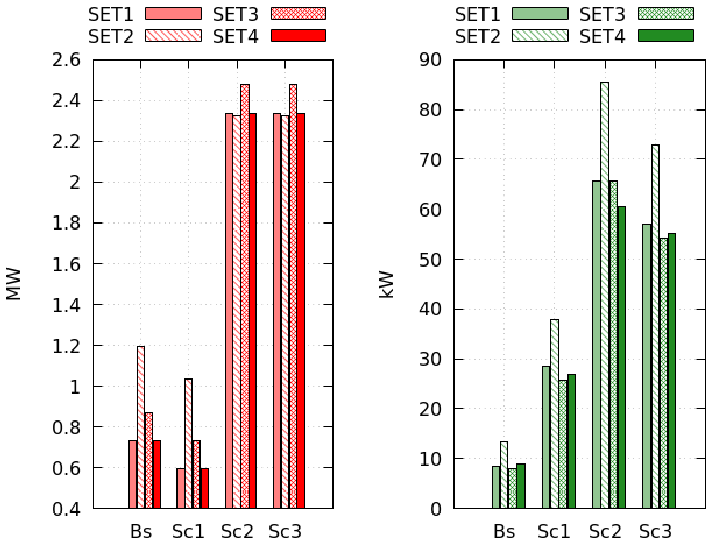
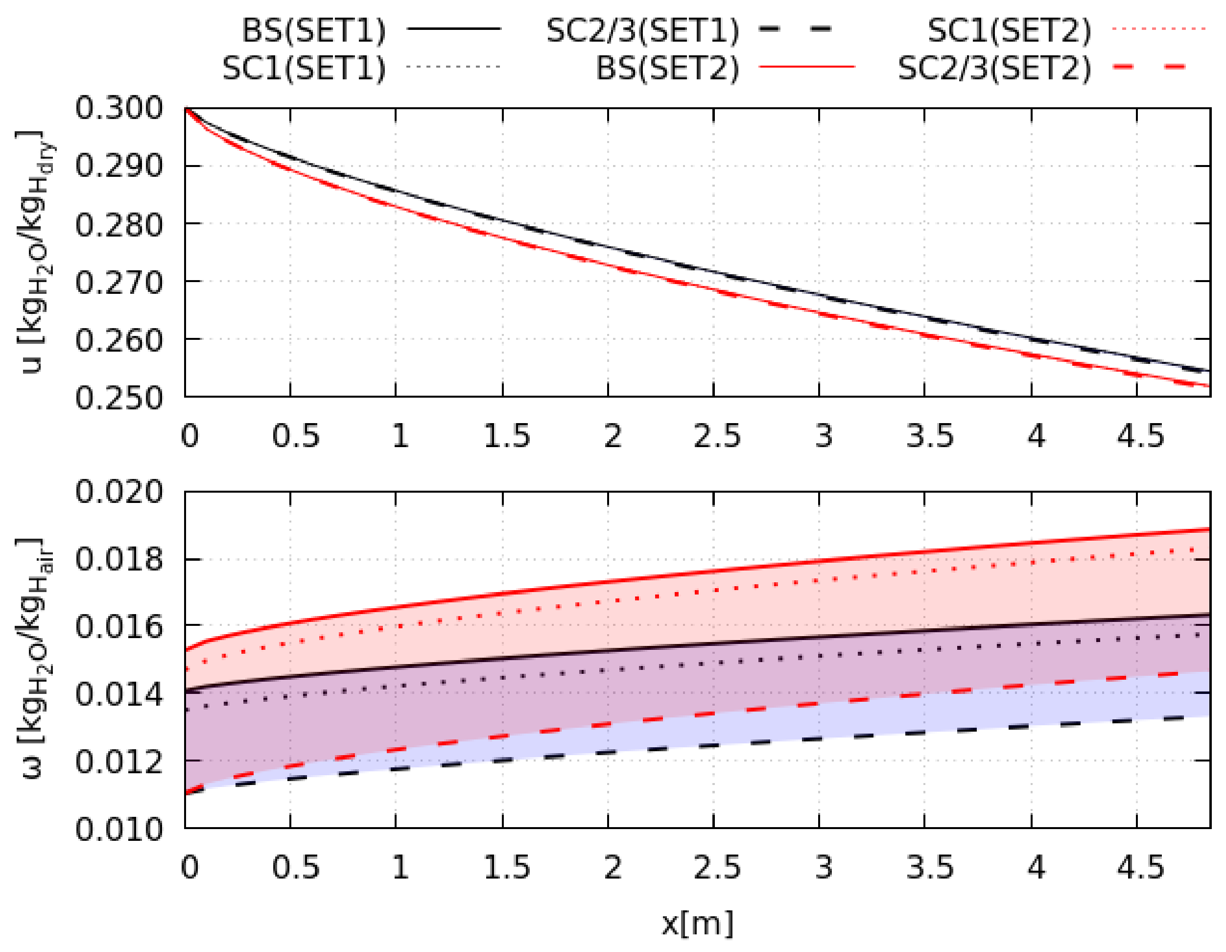
On comparing the results of different $sets$ to the reference $set1$, the evaporation rate showed the most significant effect on the global performance because it determines the energy and exergy productively invested in the drying process. When increasing heating and flowing loads ($set2$), the system evaporates a deeper moisture layer with benefits on the exergy efficiency (+97%). Higher initial product moisture ($set3$) augments the evaporation rate, and the drying cycles presents the best performance in terms of drying efficiency (+114%) and exergy efficiency (+127%). When drying the MSS ($set4$), the evaporation rate reduces by approximately ${10}^2$ times, worsening the exergy performance (−97%); such results reveal the dimensions of the drying bed inadequate to dry that particular product.

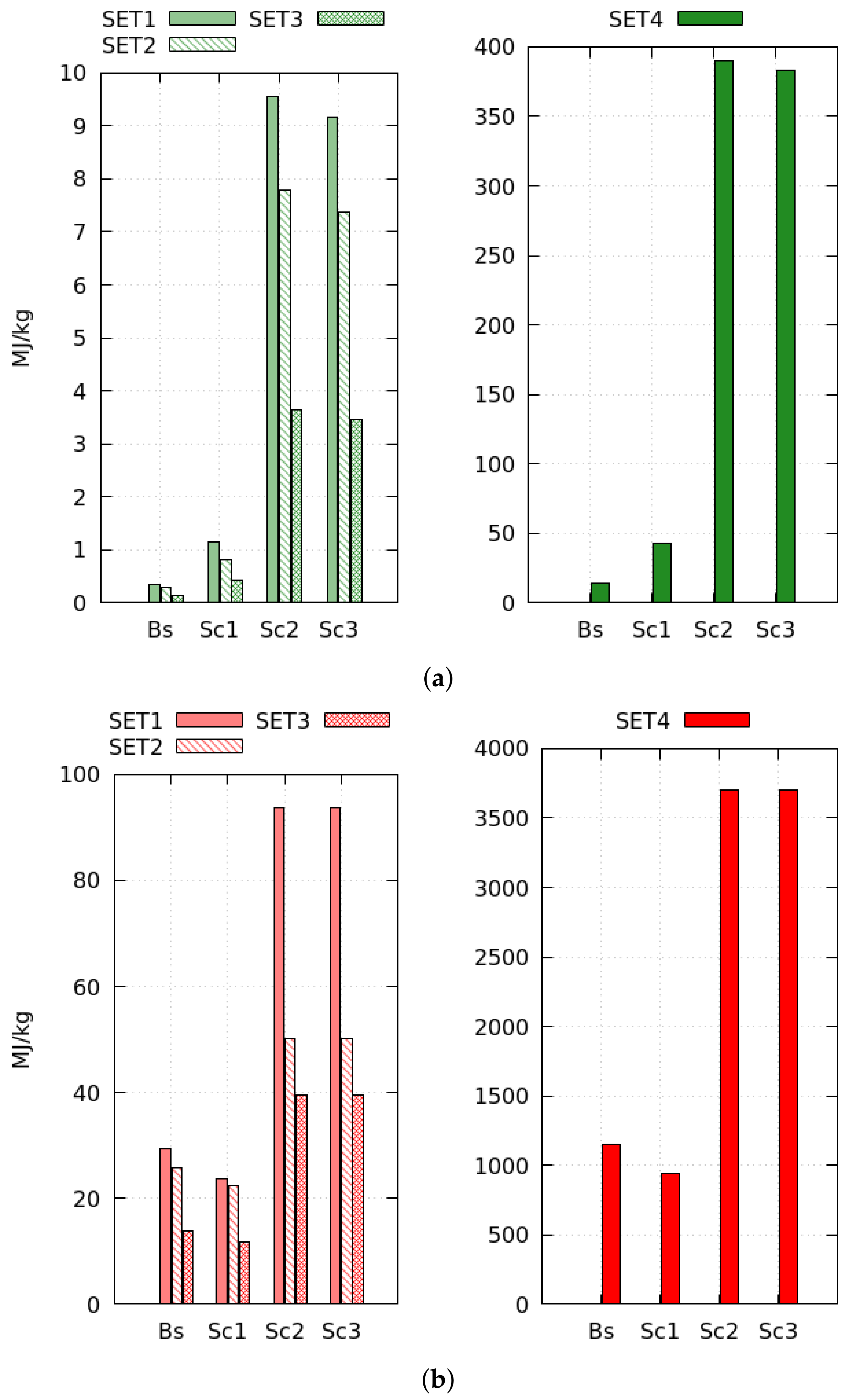
Scenario 1 is the optimal system configuration. The heat-recovery increases the baseline electrical consumption and reduces the thermal consumption by maximum +211% and −17%, respectively, with benefits on the exergy efficiency (+17%). The efficiency of heat recovery depends on the wasted energy; at low drying efficiency, or when the fan dissipates more shaft work, the HE1 fulfills the production target reducing the exchange surface by 25%. Thus, the heat-recovery is more convenient in low efficiency processes when the material is difficult to dry.

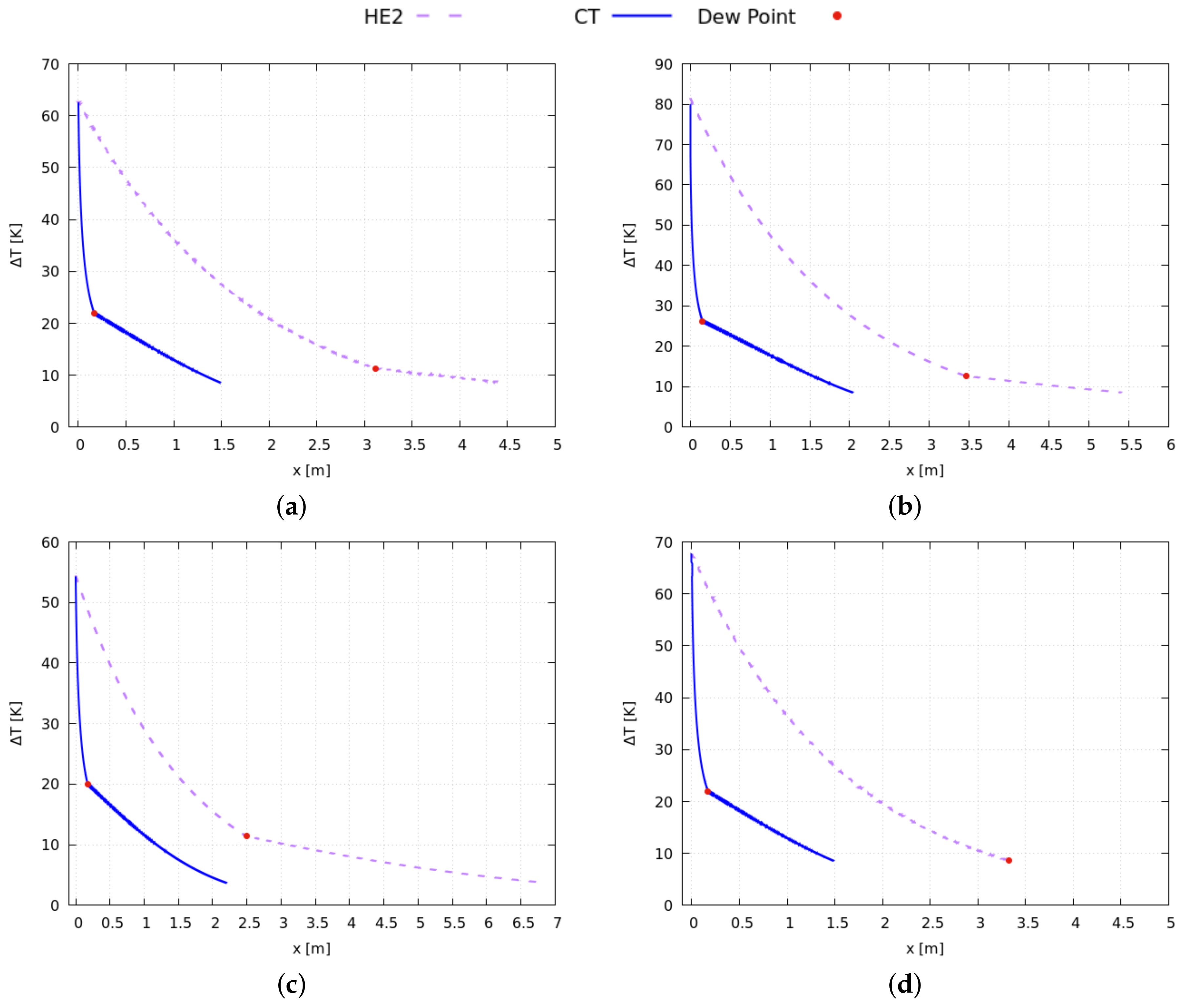
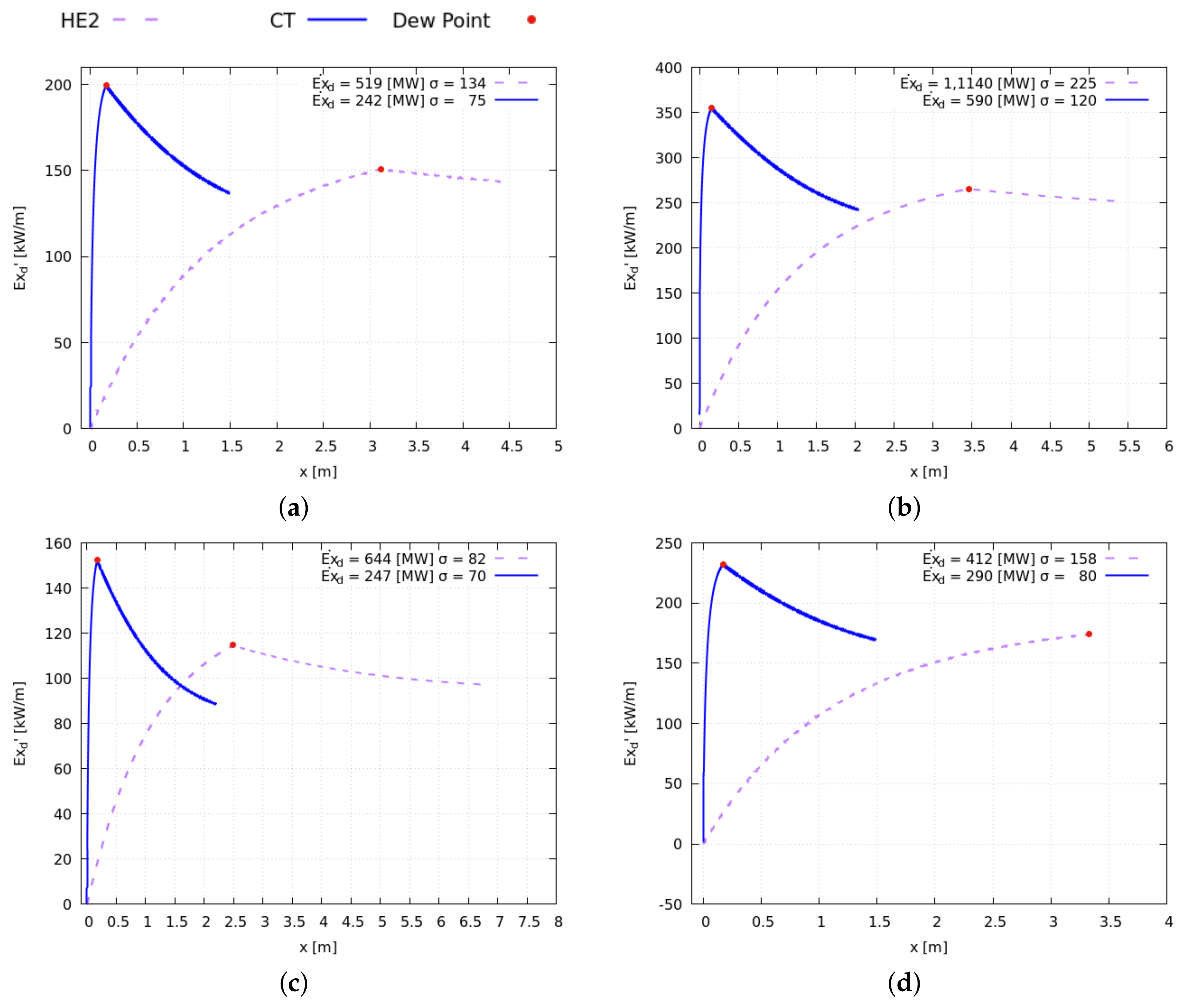
Closed cycles cut the exergy efficiency by maximum −67%. These systems use four additional heat exchangers increasing the electric consumption by 20 times. Moreover, external combustion and air regeneration processes augment the thermal energy needs (+180%). The performances of Scenario 3 are slightly better than that of Scenario 2 because the tower presents a faster cooling-rate than HE2, especially in the saturation step. This process occurs almost instantaneously in the tower that reaches the target cooling conditions with a 10 times smaller surface than HE2. Furthermore, when the saturation step becomes shorter, the total exergy destruction rate diminishes (−48%), and its spatial distribution tends to become more uniform (−39%). Thus, the tower reduces system irreversibility.

Based on the above results, we derive some technical recommendations that can help the designer optimize the energy and exergy use of a convective drying system.

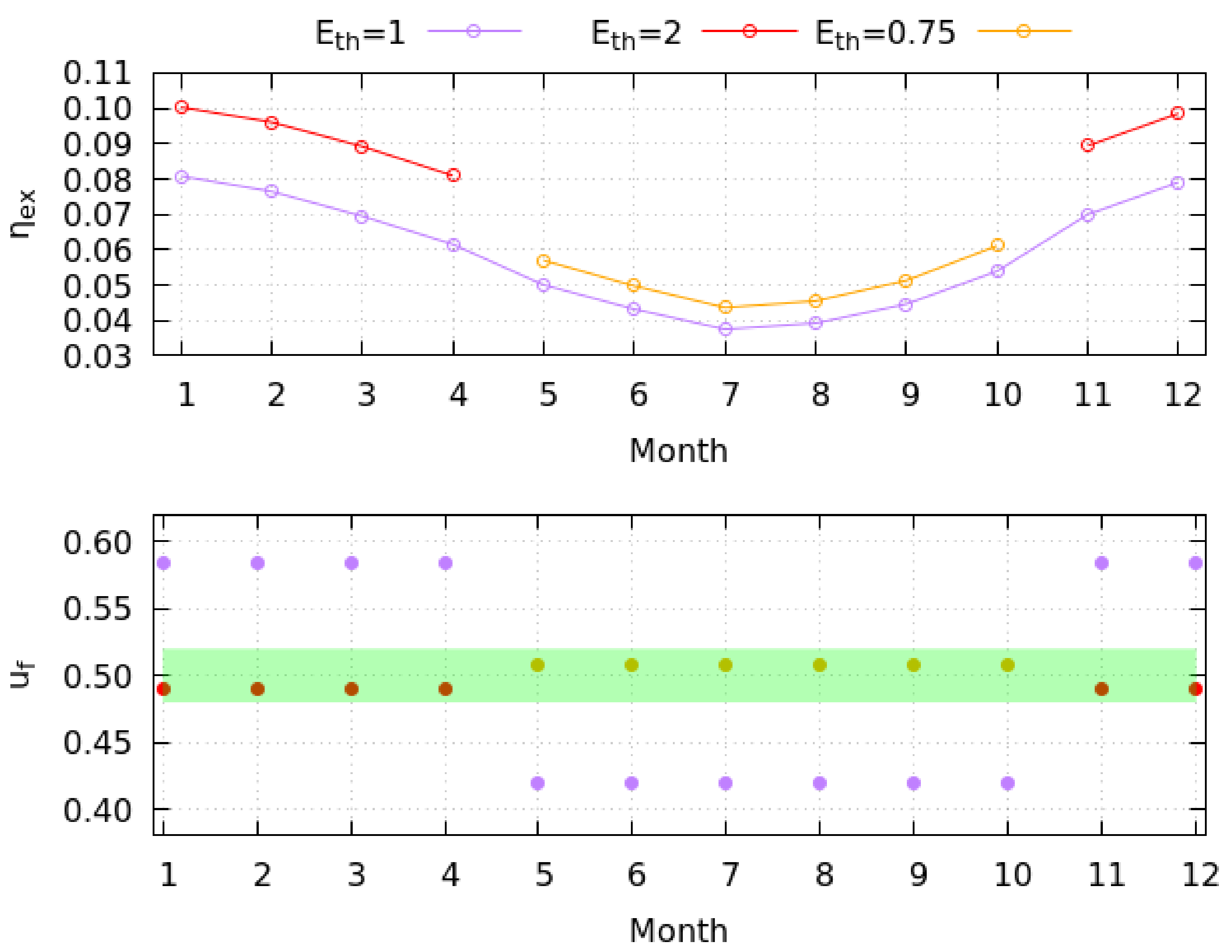
• The performance of the system varies along the climatic year because of the variations of the initial temperature and humidity of the working flows (air intake and processed product). However, the designer can ensure the production targets are unaltered by adjusting the energy input with benefits on the exergy efficiency. Best performances are observed in the cold season.
• Operating conditions shall be oriented to maximize the evaporation rate; the increasing thermal loads is valid to this purpose; however, it is limited by some adverse effects as the depletion of the product quality and the humidification of drying air by combustion. As an alternative, the designer can augment the dimensions of the drying bed and extend the residence time of the processed product in the drying chamber.
• When the bed cannot be enlarged, the drying efficiency is low, and a heat recovery unit can reuse a fraction of the heat wasted by the drying chamber to preheat the external air intake; this practice is particularly advantageous in high-temperature processes where small units significantly increase energy and exergy efficiency.
• Air recirculation dramatically reduces the performance of the system because of air regeneration processes. More than an optimization practice, the cycle closure can be a safety procedure for drying hazardous materials and limit the emissions of harmful substances in the environment. The cooling tower is particularly suitable for this purpose; compared to an indirect cooling system, it presents the highest energy and exergy efficiency and is configurable as a wet scrubber to wash away toxic species from the airflow and restore its initial conditions.

Future developments will overcome the limitations of the current work. Using a real gas model (e.g., Van der Walls), the TFMM can simulate the compression and throttle of a refrigerant fluid and predict the performances of a drying cycle driven by the heat pump, thereby promising remarkable enhancement of the exergy efficiency caused by the low-temperature of the heat generation process. Finally, the coupling of the TFMM to an analytical model (e.g., upscaled porosity model) will increase the accuracy of TFMM to describe the drying phenomenology and simulate the process at a higher level of detail.

References

1. Lewis, W.K. The rate of drying of solid materials. Ind. Eng. Chem. 1921, 13, 427–432. [Google Scholar] [CrossRef]
2. Castro, A.; Mayorga, E.; Moreno, F. Mathematical modelling of convective drying of fruits: A review. J. Food Eng. 2018, 223, 152–167. [Google Scholar] [CrossRef]
3. Mikhailov, M.; Shishedjiev, B. Temperature and moisture distributions during contact drying of a moist porous sheet. Int. J. Heat Mass Transf. 1975, 18, 15–24. [Google Scholar] [CrossRef]
4. Sandu, C. Infrared radiative drying in food engineering: A process analysis. Biotechnol. Prog. 1986, 2, 109–119. [Google Scholar] [CrossRef]
5. Behjat, Y.; Shahhosseini, S.; Hashemabadi, S.H. CFD modeling of hydrodynamic and heat transfer in fluidized bed reactors. Int. Commun. Heat Mass Transf. 2008, 35, 357–368. [Google Scholar] [CrossRef]
6. Alagha, M.S.; Szentannai, P. Analytical review of fluid-dynamic and thermal modeling aspects of fluidized beds for energy conversion devices. Int. J. Heat Mass Transf. 2020, 147, 118907. [Google Scholar] [CrossRef]
7. Daud, W.R.W. Fluidized bed dryers—Recent advances. Adv. Powder Technol. 2008, 19, 403–418. [Google Scholar] [CrossRef]
8. Turchiuli, C.; Smail, R.; Dumoulin, E. Fluidized bed agglomeration of skim milk powder: Analysis of sampling for the follow-up of agglomerate growth. Powder Technol. 2013, 238, 161–168. [Google Scholar] [CrossRef]
9. Kemp, I.C. Fundamentals of energy analysis of dryers. Mod. Dry. Technol. 2012, 4, 1–46. [Google Scholar]
10. Erbay, Z.; Hepbasli, A. Exergoeconomic evaluation of a ground-source heat pump food dryer at varying dead state temperatures. J. Clean. Prod. 2017, 142, 1425–1435. [Google Scholar] [CrossRef]
11. Milota, M.; Mosher, P. Emissions of hazardous air pollutants from lumber drying. Facilities 2007, 58, 50–55. [Google Scholar]
12. Deng, W.Y.; Yan, J.H.; Li, X.D.; Wang, F.; Zhu, X.W.; Lu, S.Y.; Cen, K.F. Emission characteristics of volatile compounds during sludges drying process. J. Hazard. Mater. 2009, 162, 186–192. [Google Scholar] [CrossRef] [PubMed]
13. Liu, W.; Xu, J.; Liu, J.; Cao, H.; Huang, X.F.; Li, G. Characteristics of ammonia emission during thermal drying of lime sludge for co-combustion in cement kilns. Environ. Technol. 2015, 36, 226–236. [Google Scholar] [CrossRef] [PubMed]
14. Tsatsaronis, G. Recent developments in exergy analysis and exergoeconomics. Int. J. Exergy 2008, 5, 489–499. [Google Scholar] [CrossRef]
15. Syahrul, S.; Hamdullahpur, F.; Dincer, I. Thermal analysis in fluidized bed drying of moist particles. Appl. Therm. Eng. 2002, 22, 1763–1775. [Google Scholar] [CrossRef]
16. Tohidi, M.; Sadeghi, M.; Torki-Harchegani, M. Energy and quality aspects for fixed deep bed drying of paddy. Renew. Sustain. Energy Rev. 2017, 70, 519–528. [Google Scholar] [CrossRef]
17. Dincer, I.; Sahin, A. A new model for thermodynamic analysis of a drying process. Int. J. Heat Mass Transf. 2004, 47, 645–652. [Google Scholar] [CrossRef]
18. Akpinar, E.K. Thermodynamic analysis of strawberry drying process in a cyclone type dryer. J. Sci. Ind. Res. 2007, 66, 152–161. [Google Scholar]
19. Yogendrasasidhar, D.; Setty, Y.P. Drying kinetics, exergy and energy analyses of Kodo millet grains and Fenugreek seeds using wall heated fluidized bed dryer. Energy 2018, 151, 799–811. [Google Scholar] [CrossRef]
20. Aviara, N.A.; Onuoha, L.N.; Falola, O.E.; Igbeka, J.C. Energy and exergy analyses of native cassava starch drying in a tray dryer. Energy 2014, 73, 809–817. [Google Scholar] [CrossRef]
21. Icier, F.; Colak, N.; Erbay, Z.; Kuzgunkaya, E.H.; Hepbasli, A. A comparative study on exergetic performance assessment for drying of broccoli florets in three different drying systems. Dry. Technol. 2010, 28, 193–204. [Google Scholar] [CrossRef] [Green Version]
22. Xiang, F.; Wang, L.; Yue, X.F. Exergy analysis and experimental study of a vehicle-mounted heat pump–assisted fluidization drying system driven by a diesel generator. Dry. Technol. 2011, 29, 1313–1324. [Google Scholar] [CrossRef]
23. Cay, A.; Tarakçıoğlu, I.; Hepbasli, A. Exergetic analysis of textile convective drying with stenters by subsystem models: Part 1—Exergetic modeling and evaluation. Dry. Technol. 2010, 28, 1359–1367. [Google Scholar] [CrossRef]
24. Cay, A.; Tarakçıoğlu, I.; Hepbasli, A. Exergetic analysis of textile convective drying with stenters by subsystem models: Part 2—Parametric study on exergy analysis. Dry. Technol. 2010, 28, 1368–1376. [Google Scholar] [CrossRef]
25. Gungor, A.; Erbay, Z.; Hepbasli, A. Exergoeconomic analyses of a gas engine driven heat pump drier and food drying process. Appl. Energy 2011, 88, 2677–2684. [Google Scholar] [CrossRef]
26. Meyer, L.; Tsatsaronis, G.; Buchgeister, J.; Schebek, L. Exergoenvironmental analysis for evaluation of the environmental impact of energy conversion systems. Energy 2009, 34, 75–89. [Google Scholar] [CrossRef]
27. Morosuk, T.; Tsatsaronis, G. Advanced exergy-based methods used to understand and improve energy-conversion systems. Energy 2019, 169, 238–246. [Google Scholar] [CrossRef]
28. Tsatsaronis, G. Thermoeconomic analysis and optimization of energy systems. Prog. Energy Combust. Sci. 1993, 19, 227–257. [Google Scholar] [CrossRef]
29. Gidaspow, D. Multiphase Flow and Fluidization: Continuum and Kinetic Theory Descriptions; Academic Press: Cambridge, MA, USA, 1994. [Google Scholar]
30. Defraeye, T. Advanced computational modelling for drying processes–A review. Appl. Energy 2014, 131, 323–344. [Google Scholar] [CrossRef]
31. Ramachandran, R.P.; Akbarzadeh, M.; Paliwal, J.; Cenkowski, S. Computational fluid dynamics in drying process modelling—A technical review. Food Bioprocess Technol. 2018, 11, 271–292. [Google Scholar] [CrossRef]
32. Assari, M.; Tabrizi, H.B.; Saffar-Avval, M. Numerical simulation of fluid bed drying based on two-fluid model and experimental validation. Appl. Therm. Eng. 2007, 27, 422–429. [Google Scholar] [CrossRef]
33. Assari, M.; Tabrizi, H.B.; Najafpour, E. Energy and exergy analysis of fluidized bed dryer based on two-fluid modeling. Int. J. Therm. Sci. 2013, 64, 213–219. [Google Scholar] [CrossRef]
34. Li, M.; Duncan, S. Dynamic model analysis of batch fluidized bed dryers. Part. Part. Syst. Charact. 2008, 25, 328–344. [Google Scholar] [CrossRef]
35. Ranjbaran, M.; Emadi, B.; Zare, D. CFD simulation of deep-bed paddy drying process and performance. Dry. Technol. 2014, 32, 919–934. [Google Scholar] [CrossRef]
36. Rosli, M.I.; Nasir, A.; Mu’im, A.; Takriff, M.S.; Chern, L.P. Simulation of a Fluidized Bed Dryer for the Drying of Sago Waste. Energies 2018, 11, 2383. [Google Scholar] [CrossRef] [Green Version]
37. Jang, J.; Arastoopour, H. CFD simulation of a pharmaceutical bubbling bed drying process at three different scales. Powder Technol. 2014, 263, 14–25. [Google Scholar] [CrossRef]
38. Padoin, N.; Dal’Toé, A.T.; Rangel, L.P.; Ropelato, K.; Soares, C. Heat and mass transfer modeling for multicomponent multiphase flow with CFD. Int. J. Heat Mass Transf. 2014, 73, 239–249. [Google Scholar] [CrossRef]
39. Yiming, S.; Jinrong, S.; Ming, G.; Bin, C.; Yanhong, Y.; Xiaoxun, M. Modeling of Mass Transfer in Nonideal Multicomponent Mixture with Maxwell-Stefan Approach. Chin. J. Chem. Eng. 2010, 18, 362–371. [Google Scholar]
40. Cui, X.; Li, X.; Sui, H.; Li, H. Computational fluid dynamics simulations of direct contact heat and mass transfer of a multicomponent two-phase film flow in an inclined channel at sub-atmospheric pressure. Int. J. Heat Mass Transf. 2012, 55, 5808–5818. [Google Scholar] [CrossRef]
41. Defraeye, T.; Blocken, B.; Carmeliet, J. Analysis of convective heat and mass transfer coefficients for convective drying of a porous flat plate by conjugate modelling. Int. J. Heat Mass Transf. 2012, 55, 112–124. [Google Scholar] [CrossRef] [Green Version]
42. Erbay, Z.; Icier, F. A review of thin layer drying of foods: Theory, modeling, and experimental results. Crit. Rev. Food Sci. Nutr. 2010, 50, 441–464. [Google Scholar] [CrossRef] [PubMed]
43. Han, X.; Liu, M.; Zhai, M.; Chong, D.; Yan, J.; Xiao, F. Investigation on the off-design performances of flue gas pre-dried lignite-fired power system integrated with waste heat recovery at variable external working conditions. Energy 2015, 90, 1743–1758. [Google Scholar] [CrossRef]
44. Han, X.; Liu, M.; Wu, K.; Chen, W.; Xiao, F.; Yan, J. Exergy analysis of the flue gas pre-dried lignite-fired power system based on the boiler with open pulverizing system. Energy 2016, 106, 285–300. [Google Scholar] [CrossRef]
45. Manente, G.; Toffolo, A.; Lazzaretto, A.; Paci, M. An Organic Rankine Cycle off-design model for the search of the optimal control strategy. Energy 2013, 58, 97–106. [Google Scholar] [CrossRef]
46. Ypma, T.J. Historical development of the Newton–Raphson method. SIAM Rev. 1995, 37, 531–551. [Google Scholar] [CrossRef] [Green Version]
47. Mohapatra, D.; Bal, S. Determination of Specific Heat and Gelatinization Temperature of Rice using Differential Scanning Calorimetry. In Proceedings of the 2003 ASAE Annual Meeting, Las Vegas, NV, USA, 27–30 July 2003; American Society of Agricultural and Biological Engineers: St. Joseph, MI, USA, 2003; p. 1. [Google Scholar]
48. Faitli, J.; Magyar, T.; Erdélyi, A.; Murányi, A. Characterization of thermal properties of municipal solid waste landfills. Waste Manag. 2015, 36, 213–221. [Google Scholar] [CrossRef]
49. Gyftopoulos, E.P.; Beretta, G.P. Thermodynamics: Foundations and Applications; Courier Corporation: Chelmsford, MA, USA, 2005. [Google Scholar]
50. Sarker, M.; Ibrahim, M.; Aziz, N.A.; Punan, M. Application of simulation in determining suitable operating parameters for industrial scale fluidized bed dryer during drying of high impurity moist paddy. J. Stored Prod. Res. 2015, 61, 76–84. [Google Scholar] [CrossRef]
51. Sarker, M.S.H.; Ibrahim, M.N.; Aziz, N.A.; Punan, M.S. Energy and exergy analysis of industrial fluidized bed drying of paddy. Energy 2015, 84, 131–138. [Google Scholar] [CrossRef]
52. da Silva, F.R.G.B.; de Souza, M.; da Costa, A.M.D.S.; de Matos Jorge, L.M.; Paraíso, P.R. Experimental and numerical analysis of soybean meal drying in fluidized bed. Powder Technol. 2012, 229, 61–70. [Google Scholar] [CrossRef]
53. Prachayawarakorn, S.; Tia, W.; Poopaiboon, K.; Soponronnarit, S. Comparison of performances of pulsed and conventional fluidised-bed dryers. J. Stored Prod. Res. 2005, 41, 479–497. [Google Scholar] [CrossRef]
54. Wetchacama; Soponronnarit; Wangi. Mathematical Model for Industrial Fluidized Bed Dryer. In Proceedings of the 18th ASEAN Seminar on Grain Post Harvest Technology, Manila, Philippines, 11–13 March 1997. [Google Scholar]
55. Sun, G.; Chen, M.; Huang, Y. Evaluation on the air-borne ultrasound-assisted hot air convection thin-layer drying performance of municipal sewage sludge. Ultrason. Sonochem. 2017, 34, 588–599. [Google Scholar] [CrossRef] [PubMed]
56. Rosen, M.A.; Dincer, I. Exergy analysis of waste emissions. Int. J. Energy Res. 1999, 23, 1153–1163. [Google Scholar] [CrossRef]
57. McDonald, A.; Dare, P.; Gifford, J.; Steward, D.; Riley, S. Assessment of air emissions from industrial kiln drying of Pinus radiata wood. Holz Als Roh-Und Werkst. 2002, 60, 181–190. [Google Scholar] [CrossRef]
58. de Gouw, J.A.; Howard, C.J.; Custer, T.G.; Fall, R. Emissions of volatile organic compounds from cut grass and clover are enhanced during the drying process. Geophys. Res. Lett. 1999, 26, 811–814. [Google Scholar] [CrossRef]
59. Mistry, K.H.; Zubair, S.M. Effect of entropy generation on the performance of humidification-dehumidification desalination cycles. Int. J. Therm. Sci. 2010, 49, 1837–1847. [Google Scholar] [CrossRef] [Green Version]
60. Tondeur, D.; Kvaalen, E. Equipartition of entropy production. An optimality criterion for transfer and separation processes. Ind. Eng. Chem. Res. 1987, 26, 50–56. [Google Scholar] [CrossRef]
61. Goshayshi, H.; Missenden, J. The investigation of cooling tower packing in various arrangements. Appl. Therm. Eng. 2000, 20, 69–80. [Google Scholar] [CrossRef]
62. Xu, Z.; Wang, R.; Yang, C. Perspectives for low-temperature waste heat recovery. Energy 2019, 176, 1037–1043. [Google Scholar] [CrossRef]
63. Ertekin, C.; Firat, M.Z. A comprehensive review of thin-layer drying models used in agricultural products. Crit. Rev. Food Sci. Nutr. 2017, 57, 701–717. [Google Scholar] [CrossRef]
64. Thiel, G.P. Entropy generation in condensation in the presence of high concentrations of noncondensable gases. Int. J. Heat Mass Transf. 2012, 55, 5133–5147. [Google Scholar] [CrossRef] [Green Version]
65. Macdonald, I.; El-Sayed, M.; Mow, K.; Dullien, F. Flow through porous media-the Ergun equation revisited. Ind. Eng. Chem. Fundam. 1979, 18, 199–208. [Google Scholar] [CrossRef]
66. Houghton, J.I.; Burgess, J.E.; Stephenson, T. Off-line particle size analysis of digested sludge. Water Res. 2002, 36, 4643–4647. [Google Scholar] [CrossRef] [Green Version]
67. Soponronnarit, S. Fluidized bed paddy drying. Sci. Asia 1999, 25, 51–56. [Google Scholar] [CrossRef]
68. Chandran, A.; Rao, S.S.; Varma, Y. Fluidized bed drying of solids. AIChE J. 1990, 36, 29–38. [Google Scholar] [CrossRef]
69. Bizmark, N.; Mostoufi, N.; Sotudeh-Gharebagh, R.; Ehsani, H. Sequential modeling of fluidized bed paddy dryer. J. Food Eng. 2010, 101, 303–308. [Google Scholar] [CrossRef]
70. Kakac, S.; Liu, H.; Pramuanjaroenkij, A. Heat Exchangers: Selection, Rating, and Thermal Design; CRC Press: Boca Raton, FL, USA, 2020. [Google Scholar]
71. Oǧulata, R.T. Utilization of waste-heat recovery in textile drying. Appl. Energy 2004, 79, 41–49. [Google Scholar] [CrossRef]
72. Aktaş, M.; Şevik, S.; Amini, A.; Khanlari, A. Analysis of drying of melon in a solar-heat recovery assisted infrared dryer. Sol. Energy 2016, 137, 500–515. [Google Scholar] [CrossRef]
73. El Fil, B.; Garimella, S. Waste Heat Recovery in Commercial Gas-Fired Tumble Dryers. Energy 2020, 218, 119407. [Google Scholar] [CrossRef]
74. Felli, M. Lezioni di Fisica Tecnica II (Energetica-Meccanica)-Trasmissione del Calore, Acustica, Tecnica Dell’illuminazione; Morlacchi Editore: Perugia, Italy, 2004. [Google Scholar]
75. Beale, S.B. Fluid Flow and Heat Transfer in Tube Banks. Ph.D. Thesis, Imperial College London (University of London), London, UK, 1992. [Google Scholar]
76. UNI EN 14551:2018-1: Air Conditioners, Liquid Chilling Packages and Heat Pumps for Space Heating and Cooling and Process Chillers, with Electrically Driven Compressors-Part 1: Terms and Definitions; Ente Nazionale Italiano di Unificazione (UNI): Milano, Italy, 2018.
77. Buck, A.L. New equations for computing vapor pressure and enhancement factor. J. Appl. Meteorol. 1981, 20, 1527–1532. [Google Scholar] [CrossRef] [Green Version]
78. Osterle, F. On the analysis of counter-flow cooling towers. Int. J. Heat Mass Transf. 1991, 34, 1313–1316. [Google Scholar] [CrossRef]
Figure 1. Fluidized bed drying chamber: (1) product inlet; (2) air inlet; (3) air diffuser; (4) conveyor belt; (5) insulated wall; (6) air outlet; and (7) product outlet.
Energies 14 00223 g001
Figure 2. The two-fluid multispecies model of the i-phase formed by the dispersed j-species.
Energies 14 00223 g002
Figure 3. Solving algorithm applied to the baseline scenario.
Energies 14 00223 g003
Figure 4. Baseline scenario corresponds to the layout of the case study.
Energies 14 00223 g004
Figure 5. Simulation vs. experimental data: u f (a) and T E (b) of the case study; values on the dot lines represent a prediction error of ± 10 % .
Energies 14 00223 g005
Figure 6. Value of u f under off-design conditions of rice (a) and MSS (b); values on the dot lines present the prediction error of ± 10 % .
Energies 14 00223 g006
Figure 7. Scenario 1 is the first upgrade of the baseline scenario: An open cycle installed with a heat recovery unit.
Energies 14 00223 g007
Figure 8. The spacing between the lines (L) and columns (C) of tube banks is equal in the horizontal and vertical direction s x , s y ; in air-to-air units (a,b) tubes are free and in air-to-water units (c,d) they are connected in a serpentine.
Energies 14 00223 g008
Figure 9. Closed cycles are Scenarios 2 (a) and 3 (b): An external combustion system keeps the chemical composition of the drying air unaltered; the latter is regenerated at the initial conditions by a cooling and a post-heating unit.
Energies 14 00223 g009
Figure 10. The heating (red) and flowing loads (green).
Energies 14 00223 g010
Figure 11. Moisture content of the product (a), air temperature (b), absolute humidity (c), and cumulative evaporation rate (d) along the bed length.
Energies 14 00223 g011
Figure 12. Drying efficiency η d c .
Energies 14 00223 g012
Figure 13. Effects of combustion on the u and ω values compared among different sets and scenarios.
Energies 14 00223 g013
Figure 14. Total exchange surfaces varying among the different sets and scenarios.
Energies 14 00223 g014
Figure 15. The temperature difference between two phases inside HE2 and the cooling tower (CT); the dew point (red point) separates the saturation from the condensation step: SET1 (a), SET2 (b), SET3 (c), and SET4 (d).
Energies 14 00223 g015
Figure 16. Specific electric energy consumption (SEEC) (a) and the specific thermal energy consumption (STEC) (b) collected by operative sets.
Energies 14 00223 g016
Figure 17. Exergy efficiency among different sets and scenarios.
Energies 14 00223 g017
Figure 18. Exergy destroyed in different cycles by flowing (Fan1-Fan2), heating (CC), drying (DC), and heat and mass recovery (HE-CT) processes.
Energies 14 00223 g018
Figure 19. Spatial distribution of exergy destruction rate within HE2 (purple) and cooling tower (blue); the dew point (red point) separates the saturation from the condensation step: SET1 (a), SET2 (b), SET3 (c), and SET4 (d).
Energies 14 00223 g019
Figure 20. The exergy efficiency and final moisture content of the baseline scenario in the Brescia climate year 2018 at different operating conditions; starting from inputs of set1 (data in purple), we doubled (data in red) and reduced by 25% (data in orange) the thermal loads.
Energies 14 00223 g020