Modeling and Hourly Time-Scale Characterization of the Main Energy Parameters of Parabolic-Trough Solar Thermal Power Plants Using a Simplified Quasi-Dynamic Model

Abstract

A simplified mathematical model of parabolic-trough solar thermal power plants, which allow one to carry out an energetic characterization of the main thermal parameters that influence the solar field performance, was evaluated through a comparison of simulation results. Two geographical locations were selected to evaluate the mathematical model proposed in this work—one in each hemisphere—and design considerations according with the practical/operational experience were taken. Furthermore, independent simulations were performed using the System Advisor Model (SAM) software, their results were compared with those obtained by the simplified model. According with the above, the mathematical model allows one to carry out simulations with a high degree of flexibility and adaptability, in which the equations that allow the plant to be energetically characterized are composed of a series of logical conditions that help identify boundary conditions between dawn and sunset, direct normal irradiance transients, and when the thermal energy storage system must compensate the solar field energy deficits to maintain the full load operation of the plant. Due to the above, the developed model allows one to obtain satisfactory simulation results; referring to the net electric power production, this model provides results in both hemispheres with a relative percentage error in the range of [0.28–8.38%] compared with the results obtained with the SAM, with mean square values of 4.57% and 4.21% for sites 1 and 2, respectively.

1. Introduction

The global energy demand in the first quarter of 2020 declined by 3.8%, or 150 million tons of oil equivalent (Mtoe), relative to the first quarter of 2019, reversing all of the energy demand growth of 2019 [1]. Nevertheless, it is estimated that the global energy will reach 18,608 Mtoe by 2035 [2]. For this reason, concentrating solar thermal power (CSP) plants with parabolic-trough (PT) collector technology are a feasible solution for providing coverage for part of the progressive growth of global energy demand. This is reflected by observing the commercial status of parabolic-trough solar thermal power plants (PTSTPPs), which have experienced an important growth. The worldwide installed capacity of PTSTPPs reached 4.7 GWe at the beginning of 2019, which represents a 643.7% increase between 2009 and 2019 [3], thus positioning the PT technology as the most mature CSP technology in the world.

To date, large-scale numerical-model computer simulations have been used in the design of PTSTPPs, which compute all energy flows as a function of the meteorological data and operating variables. Usually, these models are too specific and complex and do not include the complete PTSTPP, modeling only some subsystems [4]. In the same way, many simulations preclude a clear physical understanding of how the performance of the plant varies with the input and operational variables; usually, these models are based on cumbersome encoded and unalterable numerical procedures [5,6,7]. In addition, according to what is mentioned by Wei, S. et al. [8], these models are usually constructed to model the behavior of variables that are specific to solar field (SF) components of a PTSTPP, so in addition to the fact that they are rather cumbersome models and do not allow one to model a PTSTPP globally, they tend to have a high computational cost.

Due to the above, the development of mathematical models that minimize the uncertainty of results with a high degree of adaptability and that integrate international practical/operational experience is of high relevance because they help in decision-making, especially related to locations lacking this experience, and they allow the observation of the behavior of the main variables that characterize the system.

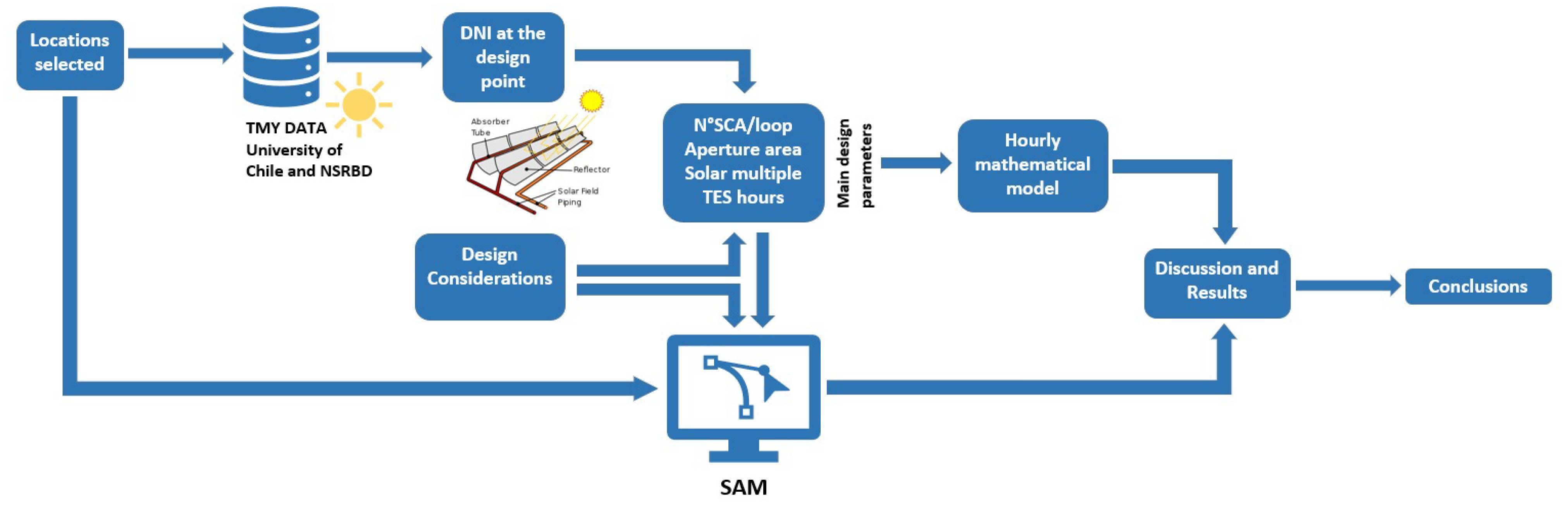
In order to solve such problems, a simplified quasi-dynamic model is presented in this paper, which allows one to model and characterize the thermal behavior of the most important parameters of the solar field (SF) of a PTSTPP (i.e., the useful thermal energy delivered by each collector loop, the useful thermal energy of the SF, the surplus thermal energy of the SF, the surplus thermal energy stored in the thermal energy storage (TES) system, and the thermal energy jointly provided by the SF and the TES) on an hourly time scale. Moreover, equations for modeling the evolution of the hourly gross and net electric power generation were developed. For the evaluation of this model, two geographical locations were selected—one in each hemisphere—of which a typical meteorological year (TMY) file was obtained to perform the simulation. The simulation results obtained with the simplified mathematical model presented in this paper and the independent simulations made with the System Advisor Model (SAM) software [9] were compared to evaluate the differences between both results and to make clear the multiple benefits of the simplified model.

The rest of this paper is organized as follows. Section 2 introduces the main concepts related with PTSTPPs; Section 3 presents the methodological procedure followed; Section 4 shows the cases under study; design conditions are mentioned in Section 5; Section 6 presents the simplified mathematical model used throughout this work; a discussion and the results are shown in Section 7, which presents the results and their comparison with the simulation results obtained with the SAM. The conclusions are given in Section 8.

The model of parabolic-trough solar thermal power plants (PTSTPPs) presented in this paper has two main innovations when compared with previous models:

• Outstanding simplification of the daily overnight thermal loss modeling by using an average plant overnight thermal loss that is calculated using the average overnight ambient temperature profile obtained from the TMY (typical meteorological year) data. This is explained in Section 7.2.
• The use of several logic functions described in Section 6 allows the plant performance simulation under transients with a very good balance between the model complexity and the accuracy of the results obtained. The logic functions proposed easily identify and take into account the boundary conditions, which would otherwise require a dynamic model. So, for instance, solar radiation changes due to dawn, sunset, or transients during sunlight hours are identified and modeled in a proper manner with easy computation. The use of these logic functions to perform quasi-dynamic plant simulations with extremely low computation requirements has not been previously reported in the literature.

2. Parabolic-Trough Solar Thermal Power Plants (PTSTPPs)

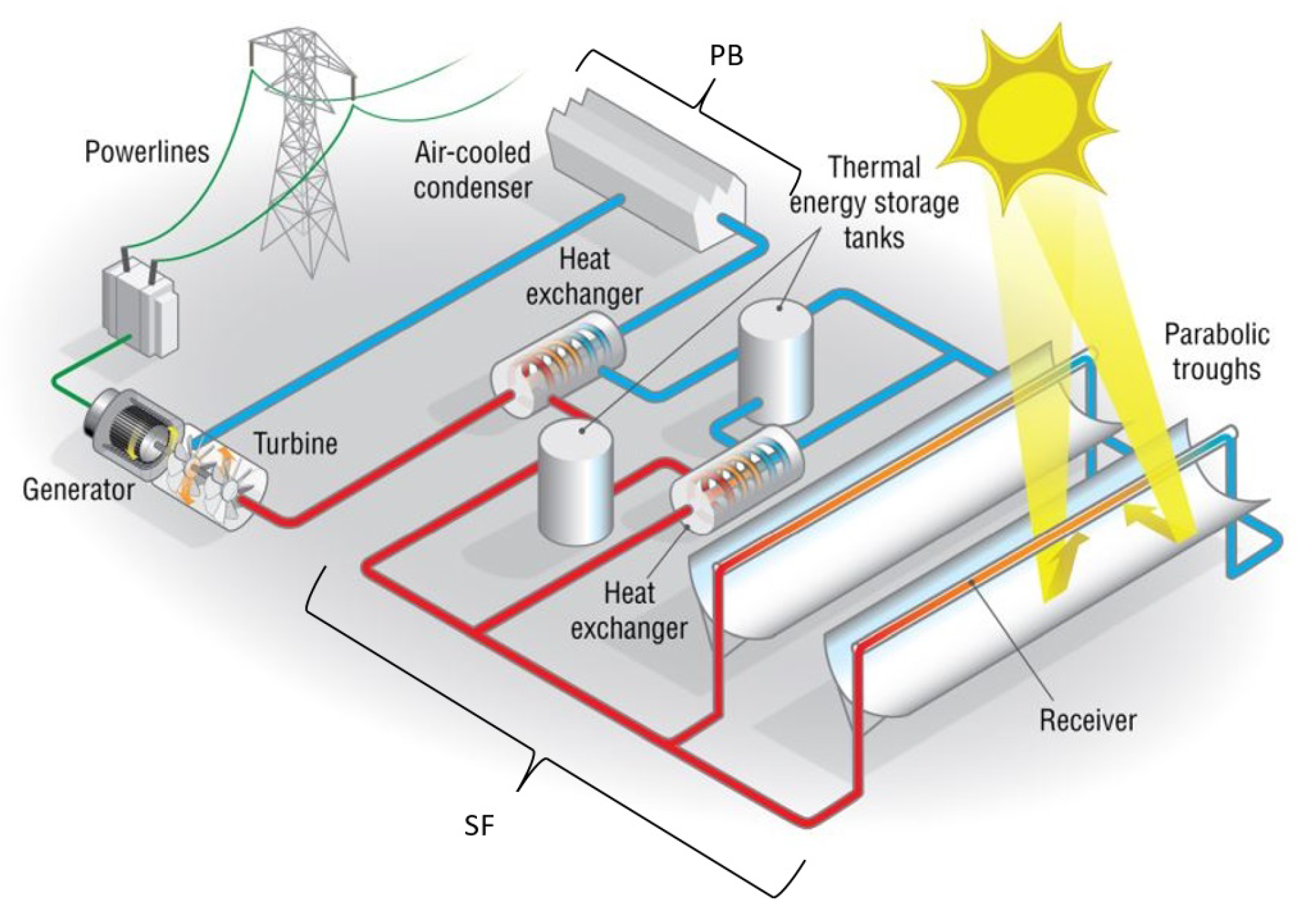
Basically, a PTSTPP is a power plant using concentrated solar radiation—specifically, the direct normal irradiance (DNI) is the primary energy source, which is concentrated and converted into thermal energy in the form of sensible or latent heat of a heat transfer fluid (HTF), which subsequently transfers this thermal energy to the power block (PB) through a set of heat exchangers for high-pressure steam generation, which is used to drive a steam turbine.

This turbine is connected to a generator that converts mechanical energy into electric energy, which is finally delivered to the external electricity grid. The concentration of the DNI in the SF is achieved by a series of parabolic mirrors that are mounted in a metal structure, thus forming the parabolic-trough collectors (PTC). These PTCs concentrate solar energy on a focal line in which a receiver tube is located to transfer heat to the HTF circulating inside [10].

A typical PTSTPP configuration is shown in Figure 1. This figure shows the main components of the SF, such as the PTCs, receiver tubes, and TES, as well as the PB. The TES is used to generate electricity in the absence of solar radiation at night and to supply the SF’s useful thermal energy deficiencies from DNI transients during sunlight hours. There are various thermal storage media, such as oil [11,12], concrete [13], sand [14], and molten salts [15]. Molten salts are currently the most commonly used in PTSTPPs. Nevertheless, the PB is the core of a PTSTPP because it must be efficient and reliable in converting thermal energy into electrical energy. The most used power blocks are based on a regenerative Rankine cycle with a super-heater (i.e., a Hirn cycle), where the main parts of the PB are a steam generation system composed of a series of heat exchangers separated in a super-heater, a re-heater, a condenser, a pre-heater, and an evaporator, as well as a cooling tower, pumps, and a turbine [16].

According to Aqachmar, Z. et al. [17], most current PTSTPPs use a synthetic thermal oil (e.g., Therminol VP-1 or Dawtherm A) as an HTF and molten salt as a thermal storage medium in the TES.

2.1. Parabolic-Trough Collectors

As mentioned in Section 2, PTCs are a type of solar concentrating collector with a linear focus that consists of a series of parabolic-shaped mirrors. These mirrors reflect and concentrate the DNI on the solar receiver placed in the focal line of the parabola. This concentrated radiation causes the HTF inside the tube to gradually be heated as it circulates inside the tube [10], thus transforming the concentrated solar radiation into thermal energy.

Table 1. General characteristics of the parabolic-trough collectors (PTCs) [18,19,20].

Parameters	Solargenix SGX2	EuroTrough ET-100	EuroTrough ET-150	SENER Trough-2
Structure	Extruded aluminum spatial structure	Support frame structure (torque box)	Support frame structure (torque box)	Stamped plates with steel torque tube
Aperture width (m)	5	5.77	5.77	6.87
Focal length (m)	1.8	1.71	1.71	2.0
Collector length (m)	100	99.5	148.5	160
Aperture area (m${}^2$)	470	545	817.5	1048
Weight (kg/m${}^2$)	22	19	18.5	-
Receiver tube’s outer diameter (m)	0.07	0.07	0.07	0.08

summarizes the characteristics of four commercial PTCs commonly used in PTSTPPs. The models ET-100 and ET-150 of the EuroTrough collector are included in Table 1, together with the model SGX2 of de compact Solargenix and the model SENERTrough developed by the Spanish company SENER.

2.2. Receiver Tube

The receiver tube is one of the most important elements in PTCs. The DNI reflected by the parabolic-shaped mirrors is concentrated onto the receiver tube, and is thus converted into thermal energy, so the overall performance of the PTC depends considerably on this element. Currently, the most widely used receiver tubes in solar thermal plants are made of two concentric tubes. The receiver tube consists of a steel tube through which the HTF circulates and an outer glass tube surrounding the steel tube. In every receiver tube, it is of real importance that the inner metal tube has a selective coating that ensures high absorptivity and low emissivity in the infrared spectrum, thus achieving high thermal performance. The glass tube covering the metal tube fulfills two important functions: to reduce the thermal losses from the convection that occurs in the metal tube and also to protect the selective coating from meteorological factors. A vacuum is made in the annular space between the steel tube and the glass tube of the receiver tube. On both sides of the glass tube, an anti-reflective treatment is made in order to have a higher transmissivity with solar radiation and also to increase the optical performance of the PTC. Most of the existing receiver tubes in the PTSTPPs currently in operation were manufactured by Schott or Siemens. It is necessary to emphasize that, the property rights of Siemens and Schott were acquired by the company Rioglass. For this reason, at present the receiver tube Schott PTR-70 is made by Rioglass in diverse factories in United State, Spain and China. [21,22].

The most widely used receiver tube model is the PTR-70 developed by the German company Schott, which includes considerable technological changes from its previous models. The main characteristics of the Schott’s PTR-70 receiver tube are shown in

Table 2. Schott PTR-70 characteristics [23].

Parameters	Schott PTR-70
Length	4.06 (m)
Metal tube’s outer diameter	70 (mm)
Glass tube’s outer diameter	125 (mm)
Selective coating	Cermet
Metal type	stainless steel
Anti-reflective treatment	Both sides
Glass type	Borosilicate
Transmittance	≥96%
Absorptivity	≥95%
Useful surface	∼95%
Emittance	≤10% at 400 ${}^{\circ }$C
Vacuum chamber	Useful life >25 years

, which was selected for the modeling of PTSTPPs with the simplified mathematical model shown in the Section 6, the object of this research.

2.3. Heat Transfer Fluids

The HTF is a fluid heated with concentrated solar radiation. Usually, thermal oils are used as HTFs in PTSTPPs. The use of molten salts as HTFs is still under development. Molten salts are commonly used in the TES as an energy storage medium by using two indirect tanks in the TES. Molten salts are always kept at a temperature above 285 ${}^{\circ }$C, thus allowing safe operation over their solidification temperature (about 245 ${}^{\circ }$C). The main HTFs available commercially are presented in

Table 3. Main heat transfer fluids (HTFs) available commercially.

HTF	Manufacturer	Composition	Operating Temperature (${}^{\circ }$C)	Price (USD/kg)
Syltherm 800	Dow Chemical	Silicon	−40 to 400	12.32
Therminol 75	Solutia	Oil	80 to 385	-
Therminol VP-1/Dow. A	Solutia	Oil	12 to 400	2.46
Hitec Xl	Coastal Chemical	48%Ca(NO${}_3$)2 7%NaNO${}_3$ 45%KNO${}_3$	150 to 500	0.78 [26]
Hitec	Coastal Chemical	40%NaNO${}_2$ 7%NaNO${}_3$ 53%KNO${}_3$	142 to 500	0.93
Solar Salt	Coastal Chemical/Soquimich	60%NaNO${}_3$ 40%KNO${}_3$	222 to 600	0.8 [27]

. Thermophysical properties are an essential factor to be considered for the efficient working of solar collectors. Regarding the above, the HTFs therminol VP-1 and Dowtherm A (synthetic oils) can withstand temperatures up to 400 ${}^{\circ }$C, but the power plant must operate above 12 ${}^{\circ }$C to avoid crystallization of the synthetic oil. Silicone-based oil Syltherm 800 can operate between −40 ${}^{\circ }$C and 400 ${}^{\circ }$C (750 ${}^{\circ }$F); however, referring to the manufacturer’s information, this HTF is too expensive, around 12.32 USD/kg compared to the 2.46 USD/kg of the Therminol VP-1. Non-eutectic nitrate molten salts (the so-called Solar Salt is composed of ${\mathrm{NaNO}}_3$:${\mathrm{KNO}}_3$ : 60:40 wt.%) must operate between 245 ${}^{\circ }$C and 600 ${}^{\circ }$C. The binary molten salt, Solar Salt, is the most common salt used as a thermal energy storage medium in CSP plants, and many research articles take solar salts as reference material in TES and heat transfer applications [24,25]. The most relevant reasons to consider for the choice of HTF are:

• The cost per kilogram of the HTF.
• The optimum operating temperature range.
• The gradual degradation of the fluid due to use.

Due to this, the HTF Therminol VP-1 and the binary salt Solar Salt were selected as HTFs in the SF and energy storage medium, respectively, for the modeling of PTSTPPs performed in this research. Thus, the main thermophysical properties of these HTFs as a function of temperature are shown in

Table 4. Correlations of HTFs’ thermophysical properties as a function of temperature [28,29].

HTF	Property	Equation	Validity Temperature Range
Therminol VP-1	Specific heat [J/kgK]	$cp=2.82T+716$	$285K<T<673K$
	Thermal Conductivity [W/mK]	$\lambda =1.73·{10}^{-7}{T}^2+7.62·{10}^{-6}T+0.14$	$285K<T<673K$
	Density kg/m${}^3$	$\rho =-7.61·{10}^{-4}{T}^{-2}-2.24·{10}^{-1}T+1191$	$285K<T<673K$
	Dynamic viscosity [Pa s]	$\mu ={(-23·{10}^{-5}{T}^3+5.61·{10}^{-3}{T}^2-19.89T+1822)}^{-1}$	$285K<T<673K$
Solar salt	Specific heat [J/kgK]	$cp=1443+0.172(T-273.15)$	$533K<T<873K$
	Thermal Conductivity [W/mK]	$\lambda =0.443+1.9·{10}^{-4}(T-273.15)$	$533K<T<873K$
	Density kg/m${}^3$	$\rho =2090-0.636(T-273.15)$	$533K<T<873K$
	Dynamic viscosity [Pa s]	$\mu =2.2714·{10}^{-2}-1.2·{10}^{-4}{(T-273.15)}^2+2.281·{10}^{-7}{(T-273.15)}^2-1.147·{10}^{-10}{(T-273.15)}^3$	$533K<T<873K$

.

3. Methodology

This section describes the methodology followed for the study described in this paper. Figure 2 shows the modeling process, which begins with the selection of a place where the solar resources from a typical meteorological year (TMY) are evaluated, from which, after an analysis of the solar resource, it is possible to obtain the day and design point for the modeling of PTSTPPs. Together with previous design considerations, hourly, monthly, and annual results are obtained. These results are compared with an independent simulation using the software system advisor model (SAM) software developed by the National Renewable Energy Laboratory (NREL), using the same parameters, such as the numbers of solar collector assemblies per loop (N ${}^{\circ }$SCA/loop), aperture area, solar multiple (SM), and TES capacity detached from the independent simplified model, and using the same design conditions. Subsequently, the discussions and conclusions are presented.

4. Cases under Study

Two geographical locations were selected for the evaluation of the PTSTPP mathematical model developed, one from each hemisphere. Geographical coordinates are shown in

Table 5. Locations selected for the case studies.

Locations	Latitude	Longitude
Southern Hemisphere (Site 1)	−24.21160	−68.7551
Northern Hemisphere (Site 2)	32.116521	−110.93304

, where the location corresponding to the Southern Hemisphere is located in the Atacama Desert, Chile, specifically in the Antofagasta region, while the location corresponding to the Northern Hemisphere is located in Tucson, in the state of Arizona (USA). The TMY data of Chile and Tucson were obtained from the solar explorer developed by the University of Chile [30] and a database already integrated in the SAM [31], respectively, to contrast the results of the simplified model with those obtained from the SAM with data from outside of this software and integrated into it.

The selected locations are shown with a satellite view in Figure 3. One of the main differences between these locations is found in the DNI indexes, which have a direct impact on the electrical energy production of PTSTPPs, as clearly evidenced in the equations presented in Section 6 and in the modeling results shown in Section 7. The site located in the Atacama Desert (see Figure 3a) has a high solar energy potential that registers an annual average of daily global horizontal irradiation (GHI) that exceeds 7.5 kWh/m${}^2$ and 9 kWh/m${}^2$ in the case of DNI, and it is also characterized by large areas of flat land [32,33,34,35]. The location selected in the state of Arizona (see Figure 3b), USA has an annual average of daily GHI and DNI that reach 5.8 kWh/m${}^2$ and 7.4 kWh/m${}^2$, respectively.

Locations with an annual DNI value of a least 2000 kWh/m${}^2$ per year have the potential to be techno-economically suitable for the implementation of CSP plants [36]. Both sites comply with this consignment, as they have 4041 kWh/m${}^2$ and 2687 kWh/m${}^2$ per year for site 1 and site 2, respectively.

5. Design Considerations

Design considerations of both plants were defined according to international practical/operational experience of PTSTPPs, such as Andasol 1-3, Solar Energy Generating Systems (SEGS) Plants, and Noor-1 [17,37,38], among others, and based on the knowledge of the authors of the present paper. As an example, the main design parameters adopted for the simulations of the plants are shown in

Table 6. Main plant design parameters considered.

Parameter	Values	Units
Nominal power	70	MWe
$T_{in}$ HTF/loop	293	${}^{\circ }$
$T_{out}$ HTF/loop	393	${}^{\circ }$
Nominal power cycle efficiency	38	%
TES–HTF heat exchanger efficiency	98	%
HTF–water heat exchanger efficiency	97	%
Soiling factor	95	%
Max. Velocity HTF feed/collection lines	2	m/s
Number of ET-100 collectors per loop	4	-
Number of loops in the SF at site 1	280	-
Number of loops in the SF at site 2	440	-
Average overnight thermal energy losses/loop at site 1	479	${\mathrm{kWh}}_{\mathrm{th}}$
Average overnight thermal energy losses/loop at site 2	320	${\mathrm{kWh}}_{\mathrm{th}}$

. Eurotrough ET-100, Schott PTR-70, Therminol VP-1, and Solar Salt were selected as the PTC, receiver tube, HTF, and molten salt, respectively [18]. Furthermore, an HTF temperature difference of 100 ${}^{\circ }$C between the inlet and outlet of each loop of the SF was considered, with HTF temperatures of 293 ${}^{\circ }$C and 393 ${}^{\circ }$C at the inlet and outlet, respectively, for both locations. In the same way, 38%, 98%, 97%, and 95% peak power cycle performance, TES–HTF heat exchanger efficiency, HTF–water heat exchanger efficiency, and soiling factor, respectively, were considered. Moreover, it is important to point out that the number of loops that compose each SF is that required on the design day to produce the thermal energy necessary for the PTSTPP to operate at full load during the whole day (24 h).

It is necessary to emphasize that the efficiency parameters assumed correspond to the efficiencies at full load operation, which are used throughout the investigation. However, in the mathematical model presented in Section 6, these parameters can be replaced by daily evaluated operational parameters representing the real operational state of the plant. For the orientation of the PTSTPPs modeled, a North–South orientation with East–West tracking was selected because it is common in commercial PTSTPPs to maximize the amount of electricity produced in annual computations. Furthermore, this orientation is usually recommended for plants that are at a location with a latitude between ±46.06${}^{\circ }$ [39]. Additionally, the SF configuration was selected following the recommendations made by NREL [40], which depend directly on the SF aperture area. For an SF aperture area greater than 400,000 m${}^2$, an “H” configuration of the SF is recommended, while for an extension of less than 400,000 m${}^2$, an “I” configuration is recommended. Following this guideline, an “H configuration” was assumed for both plants, and the diameter of each piping section was determined assuming a maximum HTF speed of 2 m/s.

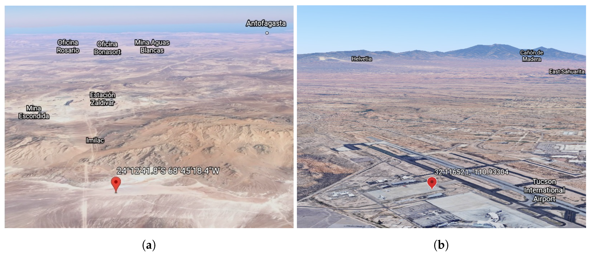
Finally, but not least, 70 MWe was taken as the nominal power for the modeled PTSTPPs. In addition, for calculating the pressure loss by the concept of pumping HTF in the SF, a roughness factor of 50 μm and 20 μm was considered for the carbon steel and stainless steel pipes, respectively. On another matter, after thoroughly analyzing the time profile of the ambient temperature integrated in the TMY data of both sites, an average overnight ambient temperature profile was defined, and average overnight thermal energy losses of 479 ${\mathrm{kWh}}_{\mathrm{th}}$ and 320 ${\mathrm{kWh}}_{\mathrm{th}}$ that must be compensated per collector loop at the beginning of the daily plant operation were obtained for sites 1 and 2, respectively (see Section 7.2). The overnight thermal energy loss to be compensated by each loop was obtained by dividing the total overnight thermal loss in the solar field by the number of loops. These values of average overnight thermal losses were calculated by taking into account the mass of the HTF and steel existing in the solar field piping and the heat capacities of the HTF and steel.

6. Mathematical Model

The mathematical model used for the modeling of PTSTPPs is presented in this section. This model was applied under the design conditions shown in Section 5. However, these parameters can be modified for any future modeling outside the framework of this research. The solar field modeling process begins by knowing the energy requests to which the solar field must respond. The thermal power at the design point that the solar field of a parabolic-trough plant must provide is conditioned by the gross electrical power of the power block, where the gross cycle efficiency ${\eta }_{cycle}$ is given by Equation (1):

$${\eta }_{cycle}=\frac{P_{e,PB}}{{\dot{Q}}_{th/PB}}$$

(1)

in which the terms $P_{e,PB}$ and ${\dot{Q}}_{th/PB}$ correspond to the gross electrical power of the power block and the thermal power required for full load operation, respectively. Likewise, to correctly characterize the solar field of PTSTPPs, the incidence angle must be determined because it directly affects the useful power delivered by each PTC. Thus, for the collector orientation selected, the cosine of the incidence angle was modeled as:

$$cos\theta =\sqrt{co{s}^2{\theta }_z+co{s}^2\delta se{n}^2\omega }$$

(2)

where the $\theta$,${\theta }_z$,$\delta$, and $\omega$ parameters correspond to the angle of incidence, zenith angle, declination angle, and hour angle, respectively. On the other hand, the zenith angle can be modeled according to the expression:

$$cos{\theta }_z=sen\delta ·sen\lambda +cos\lambda ·cos\delta ·cos\omega$$

(3)

where $\lambda$ corresponds to the latitude of the selected location. On the other hand, solar declination is computed through the next equation:

$$\delta ={23.45}^{\circ }·sen(\frac{360(dn+284)}{365})$$

(4)

where $dn$ is the Julianne Day. Therefore, the solar radiant power incident to each PTC or SCA can be modeled by the following equation:

$${\dot{Q}}_{sun/SCA}=A_c·E_b·cos\theta$$

(5)

The terms $A_c$ and $E_b$ correspond to the aperture area of the selected PTC in m${}^2$ and to the DNI at the design point in W/m${}^2$. As can be seen in Equation (5), the value of $E_b$ at the design point has a fundamental role and must correspond to a characteristic value of the site under study for the date chosen for the design day, since choosing very low design DNI values will leave part of the SF unused when the DNI values are higher than that assumed. Furthermore, the incidence angle modifier (IAM) must be modeled correctly because this parameter directly affects the DNI concentration, since it acts directly on the optical performance of each PTC. For the PTC assumed in this study (ET-100), the IAM is modeled through Equation (6).

$$k(\theta )=1-5.25097·{10}^{-4}·(\frac{\theta }{cos\theta })-2.859621·{10}^{-5}·(\frac{{\theta }^2}{cos\theta })$$

(6)

On the other hand, with the objective of determining the useful thermal power delivered by each PTC, it is essential to estimate the thermal losses from its receiver tube to the environment. Currently, there are several empirical models that allow thermal losses to be modeled for the Schott PTR-70 receiver tube, as proposed by the NREL [41]. However, Equation (7) was used in this work; it was obtained experimentally by Valenzuela, L. et al. [42] in the Plataforma Solar de Almería (PSA) for this type of receiver tube under real operating conditions, and it gives thermal losses in W/m. Thus, the value given by Equation (7) must be multiplied by the SCA length to obtain the total thermal losses, ${\dot{Q}}_{losses/SCA}$.

$${\dot{Q}}_{losses}=0.342·\Delta T+1.163·{10}^{-8}·\Delta T^4$$

(7)

Therefore, the thermal power absorbed at the receiver tubes of each SCA, ${\dot{Q}}_{abs/SCA}$, and ${\dot{Q}}_{useful/SCA}$ can be modeled by the following equations:

$${\dot{Q}}_{abs/SCA}={\dot{Q}}_{sun/SCA}·k(\theta )·{\eta }_{opt,0}·Fe$$

(8)

$${\dot{Q}}_{useful/SCA}={\dot{Q}}_{abs/SCA}-{\dot{Q}}_{losses/SCA}$$

(9)

where ${\eta }_{opt,0}$ corresponds to the peak optical efficiency of each PTC, and Fe is the soiling factor. The useful power of each solar field loop can be determined by the product between the number of SCAs connected in series in each loop, $N_{SCA/loop}^{\circ }$, and the useful power of each SCA.

$${\dot{Q}}_{useful/loop}=N_{SCA/loop}^{\circ }·{\dot{Q}}_{useful/SCA}$$

(10)

Moreover, as the TMY data come on an hourly basis, the thermal energy delivered by each loop ($E_{th,loop}$) in kWh can be determined with the product between ${\dot{Q}}_{useful/loop}$ and the elapsed time (1 h). The energy delivered by each loop in ${\mathrm{kWh}}_{\mathrm{th}}$ can be computed by Equation (11), which considers that when the DNI is null or when the DNI is not high enough to compensate for thermal losses during the day and, consequently, ${\dot{Q}}_{useful/loop}<0$, it considers these values null. That is:

$$E_{th,loo{p}_n}=\left\{\begin{array}{cc}0\hfill & \mathrm{if},DN{I}_n=0\vee ({\dot{Q}}_{useful/loo{p}_n}<0\wedge DN{I}_n>0)\hfill \\ {\dot{Q}}_{useful/loo{p}_n}·1hr\hfill & \mathrm{if},{\dot{Q}}_{useful/loo{p}_n}>0\wedge DN{I}_n>0\hfill \end{array}\right.$$

(11)

where n corresponds to a specific hour in the year, that is to say, n∈$\{1,2,3,4,5,\dots ,8760\}$. The mathematical expression shown in Equation (12) was constructed to model the useful thermal energy per loop $E_{th,useful/loo{p}_n}$ for a given hour n. This equation integrates a series of logical expressions that allow one to know when a low DNI value is due to: (a) the daily ramp up or down after sunrise and before sunset, (b) a cloudy transient taking place between sunrise and sunset, or (c) night time. Therefore, this equation takes into account the power plant start-up period, when the SF is compensating for overnight thermal losses, or when a solar transient happening during sunlight hours implies that the HTF loses temperature, so when the end of the transient is detected, the useful thermal energy delivered by each loop must compensate for energy loss of the HTF until it recovers its nominal temperature. Likewise, in Equation (12), the terms ${\eta }_{HX,system}$ and $1-{\%}_{piping,losses}$ incorporate a penalty of $E_{th,useful/loop}$ corresponding to the efficiency of the steam generator and the HTF piping that connects the SF with it. Thus, the useful thermal energy per loop can be computed as:

$$E_{th,useful/loo{p}_n}=\left\{\begin{array}{cc}({\eta }_{HX,system})·(1-{\%}_{piping,losses})·(E_{th,loo{p}_n}-{\overline{E}}_{nigth,losses})\hfill & \mathrm{if},p\hfill \\ 0\hfill & \mathrm{if},s\hfill \\ ({\eta }_{HX,system})·(1-{\%}_{piping,losses})·(E_{th,loo{p}_n}-({\overline{E}}_{nigth,losses}-E_{th,loo{p}_{n-1}}))\hfill & \mathrm{if},h\hfill \\ ({\eta }_{HX,system})·(1-{\%}_{piping,losses})·(E_{th,loo{p}_n}-{\dot{Q}}_{useful/loo{p}_{n-1}}·1hr)\hfill & \mathrm{if},t\hfill \\ ({\eta }_{HX,system})·(1-{\%}_{piping,losses})·(E_{th,loo{p}_n}+\sum _{j=n-2}^{n-1}{\dot{Q}}_{useful/loo{p}_j}·1hr)\hfill & \mathrm{if},k\hfill \\ ({\eta }_{HX,system})·(1-{\%}_{piping,losses})·(E_{th,loo{p}_n}+\sum _{j=n-3}^{n-1}{\dot{Q}}_{useful/loo{p}_j}·1hr)\hfill & \mathrm{if},q\hfill \\ ({\eta }_{HX,system})·(1-{\%}_{piping,losses})·(E_{th,loo{p}_n}+\sum _{j=n-4}^{n-1}{\dot{Q}}_{useful/loo{p}_j}·1hr)\hfill & \mathrm{if},m\hfill \\ ({\eta }_{HX,system})·(1-{\%}_{piping,losses})·(E_{th,loo{p}_n}+\sum _{j=n-5}^{n-1}{\dot{Q}}_{useful/loo{p}_j}·1hr)\hfill & \mathrm{if},r\hfill \\ .\hfill & \\ .\hfill & \\ .\hfill & \\ .\hfill & \\ ({\eta }_{HX,system})·(1-{\%}_{piping,losses})·E_{th,loo{p}_n}\hfill & \mathrm{if},u\hfill \end{array}\right.$$

(12)

where the terms p, s, h, t, k, q, m, r, and u are logical auxiliary expressions used in Equation (12). These expressions integrate a logical structure that allows one to easily identify at which moment of the day the PTSTPP is operating and, thus, model the useful thermal energy per loop in the right way. So, these expressions identify when a low value of DNI is due to the period between sunset and sunrise times or to a DNI transient during sunlight hours. They also easily identify when the solar field has already compensated for the average overnight thermal losses. Hence, in the above expression, the number of sections of the function shown in Equation (12) between the logical auxiliaries t and u depends on the time period in hours between the start and end of a DNI transitory. To do this, the evolution and temporal behavior of the DNI data integrated in the TMY file must be analyzed. It is important to note that the time behavior of the DNI is characteristic of each site. However, it has been found that for hourly data, for an instant “n” under analysis, it is sufficient to consider a time window integrating the previous seven instants of registration of the DNI to identify whether the plant is operating during the day, the night, or under a DNI transitory. Thus, these logical auxiliary expressions are computed as:

• $p={\sum }_{j=n-7}^{n-1}DN{I}_j=0\wedge E_{th,loo{p}_n}\ge {\overline{E}}_{nigth,losses}$
• $s=({\sum }_{j=n-7}^{n-1}DN{I}_j=0\wedge E_{th,loo{p}_n}<{\overline{E}}_{nigth,losses}\wedge E_{th,loo{p}_n}>0)\vee (E_{th,loo{p}_n}$$>0\wedge E_{th,loo{p}_{n-1}}=0\wedge E_{th,loo{p}_{n-2}}>0\wedge ({\eta }_{HX,system})·(1-{\%}_{piping,losses})·(E_{th,loo{p}_n}-{\dot{Q}}_{useful/loo{p}_{n-1}}·1hr)<0)$$\vee (E_{th,loo{p}_n}>0\wedge {\sum }_{j=n-2}^{n-1}{E}_{th,loo{p}_j}=0\wedge E_{th,loo{p}_{n-3}}>0\wedge ({\eta }_{HX,system})·(1-{\%}_{piping,losses})·(E_{th,loo{p}_n}+{\sum }_{j=n-2}^{n-1}{\dot{Q}}_{useful/loo{p}_j}·1hr)<0)\vee (E_{th,loo{p}_n}$$>0\wedge {\sum }_{j=n-3}^{n-1}{E}_{th,loo{p}_j}=0\wedge E_{th,loo{p}_{n-4}}>0\wedge ({\eta }_{HX,system})·(1-{\%}_{piping,losses})·(E_{th,loo{p}_n}$$+{\sum }_{j=n-3}^{n-1}{\dot{Q}}_{useful/loo{p}_j}·1hr)<0)\vee E_{th,loo{p}_n}>0\wedge {\sum }_{j=n-4}^{n-1}{E}_{th,loo{p}_j}=0\wedge E_{th,loo{p}_{n-5}}$$>0\wedge ({\eta }_{HX,system})·(1-{\%}_{piping,losses})·(E_{th,loo{p}_n}+{\sum }_{j=n-4}^{n-1}{\dot{Q}}_{useful/loo{p}_j}·1hr)$$<0\vee E_{th,loo{p}_n}>0\wedge {\sum }_{j=n-5}^{n-1}{E}_{th,loo{p}_j}=0\wedge E_{th,loo{p}_{n-6}}>0\wedge ({\eta }_{HX,system})·(1-{\%}_{piping,losses})·(E_{th,loo{p}_n}+{\sum }_{j=n-5}^{n-1}{\dot{Q}}_{useful/loo{p}_j}·1hr)<0$
• $h=E_{th,loo{p}_n}\ge {\overline{E}}_{nigth,losses}\wedge E_{th,loo{p}_{n-1}}<{\overline{E}}_{nigth,losses}\wedge E_{th,loo{p}_{n-1}}>0\wedge {\sum }_{j=n-7}^{n-2}DN{I}_j=0$
• $t=E_{th,loo{p}_n}>0\wedge E_{th,loo{p}_{n-1}}=0\wedge E_{th,loo{p}_{n-2}}>0\wedge ({\eta }_{HX,system})·(1-{\%}_{piping,losses})·(E_{th,loo{p}_n}-{\dot{Q}}_{useful/loo{p}_{n-1}}·1hr)>0$
• $k=E_{th,loo{p}_n}>0\wedge {\sum }_{j=n-2}^{n-1}{E}_{th,loo{p}_j}=0\wedge E_{th,loo{p}_{n-3}}>0\wedge ({\eta }_{HX,system})·$$(1-{\%}_{piping,losses})·(E_{th,loo{p}_n}+{\sum }_{j=n-2}^{n-1}{\dot{Q}}_{useful/loo{p}_j}·1hr)>0$
• $q=E_{th,loo{p}_n}>0\wedge {\sum }_{j=n-3}^{n-1}{E}_{th,loo{p}_j}=0\wedge E_{th,loo{p}_{n-4}}>0\wedge ({\eta }_{HX,system})·$$(1-{\%}_{piping,losses})·(E_{th,loo{p}_n}+{\sum }_{j=n-3}^{n-1}{\dot{Q}}_{useful/loo{p}_j}·1hr)>0$
• $m=E_{th,loo{p}_n}>0\wedge {\sum }_{j=n-4}^{n-1}{E}_{th,loo{p}_j}=0\wedge E_{th,loo{p}_{n-5}}>0\wedge ({\eta }_{HX,system})·$$(1-{\%}_{piping,losses})·(E_{th,loo{p}_n}+{\sum }_{j=n-4}^{n-1}{\dot{Q}}_{useful/loo{p}_j}·1hr)>0$
• $r=E_{th,loo{p}_n}>0\wedge {\sum }_{j=n-5}^{n-1}{E}_{th,loo{p}_j}=0\wedge E_{th,loo{p}_{n-6}}>0\wedge ({\eta }_{HX,system})·$$(1-{\%}_{piping,losses})·(E_{th,loo{p}_n}+{\sum }_{j=n-5}^{n-1}{\dot{Q}}_{useful/loo{p}_j}·1hr)>0$
• $u=p\wedge s\wedge h\wedge t\wedge k\wedge q\wedge m\wedge r\to False$

The number of loops composing the SF and the number of SCA in series in each loop are input data for the simulation of the PTSTPP (see Table 6). Each loop would have to compensate an average overnight thermal loss at the beginning of the daily operation of 479 kWh and 320 kWh for sites 1 and 2, respectively. As explained in Section 5, this value was calculated taking into account the average overnight ambient temperature profile at the site assumed for the plant and the mass of HTF and steel in the complete SF considering an “H” configuration. A higher overnight thermal loss should be considered for those sites with lower average overnight ambient temperatures. With the number of loops in the SF and the layout of all HTF pipes (i.e., the length and diameter of each pipe section), the quantities (kg) of steel and thermal oil throughout the SF and associated pipes, as well as the total thermal losses at night in them and in the collector loops, were calculated, considering an overnight average ambient temperature obtained from the TMY data. These total thermal losses must be compensated early in the day by the SF. Total overnight thermal losses were evenly distributed among all the loops so that the thermal energy provided by each loop in the early hours of the day is used to compensate for night thermal losses, as it is not considered as useful thermal energy for the turbine. Additionally, the shading factor per row of collectors can be modeled using the Equation (13) [43].

$$f_{shading}=min[max[0;\frac{L_{spacing}·cos{\theta }_z}{W·cos\theta };1]]$$

(13)

Where $L_{spacing}$ and W are the separation between rows of collectors and the aperture width of the selected collector, respectively. Moreover, $f_{shading}$ ∈ [0, 1], in which $f_{shading}$ values equal to 0 and 1 imply a fully shaded and shadow-free PTC, respectively, and values of $f_{shading}$ between 0 and 1 imply a partially shaded PTC.

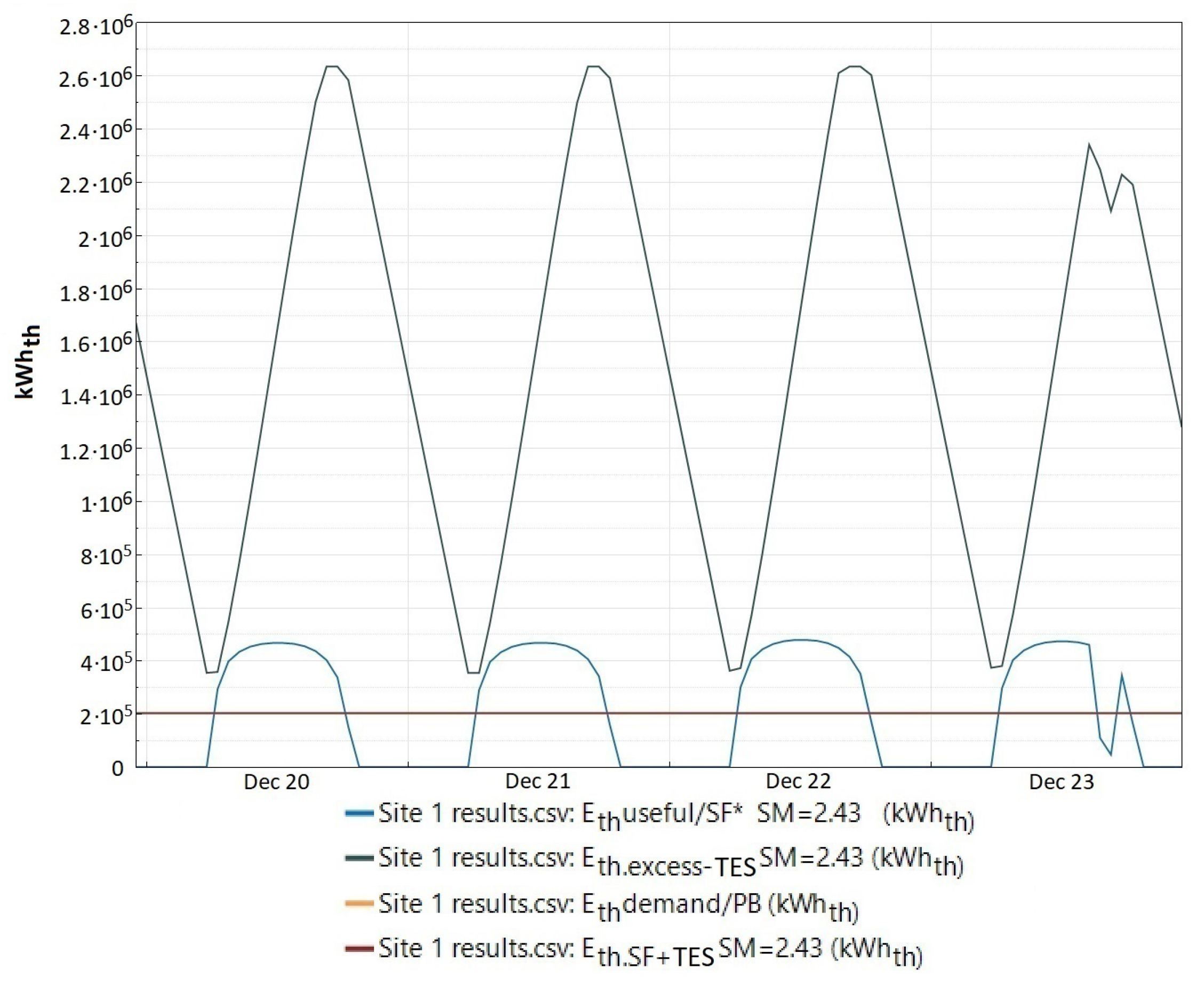
The SF’s useful hourly thermal energy in ${\mathrm{kWh}}_{\mathrm{th}}$ can be modeled as:

$$E_{th,useful-S{F}_n}=E_{th,useful/loo{p}_n}·N_{loops,SF}^{\circ }$$

(14)

Therefore, the hourly surplus SF thermal energy in ${\mathrm{kWh}}_{\mathrm{th}}$ that can be stored in the TES can be modeled by the following expression:

$$E_{th,excess-S{F}_n}=\left\{\begin{array}{cc}{E}_{th,useful-S{F}_n}-E_{th,demand-P{B}_n}\hfill & \mathrm{if},E_{th,useful-S{F}_n}>E_{th,demand-P{B}_n}\hfill \\ 0\hfill & \mathrm{if},E_{th,useful-S{F}_n}\le E_{th,demand-P{B}_n}\hfill \end{array}\right.$$

(15)

Thus, by modeling the above parameters, it is possible to determine the maximum number of hours of TES that, according to the parameters of the design day, the PTSTPP should have. Consequently, the number of hours of TES can be computed as:

$$N_{hrs,TES}^{\circ }=\frac{{\sum }_{j=1}^{24}{E}_{th,excess-S{F}_j}{|}_{dd}}{{\dot{Q}}_{th/PB}}$$

(16)

Likewise, the solar multiple (SM) of the PTSTPP can be determined by the expression shown in Equation (17), applied to the SF at the design point:

$$SM=\frac{{\dot{Q}}_{useful/loop}·N_{loops,SF}^{\circ }}{{\dot{Q}}_{th/PB}}{|}_{dp}$$

(17)

Where the term $dp$ refers to the design point. Thus, the simplified equation for modeling the quasi-dynamic charging and discharging behavior of the energy stored in the TES—to give continuity to the operation of the plant and overcome the effect of transients in the DNI, which reduces the SF’s useful thermal energy—is presented in the following expression:

$$E_{th,excess-TE{S}_n}=\left\{\begin{array}{cc}{\eta }_{HX-TES/HTF}·E_{th,excessS{F}_n}+E_{th,excess-TE{S}_{n-1}}\hfill & \mathrm{if},a\hfill \\ {\eta }_{HX-TES/HTF}·E_{th,excessS{F}_n}+E_{th,excess-TE{S}_{n-1}}-E_{th,defici{t}_n}\hfill & \mathrm{if},b\hfill \\ 0\hfill & \mathrm{si},c\hfill \\ N_{hrs,TES}^{\circ }·{\dot{Q}}_{th/PB},\hfill & \mathrm{if},d\hfill \end{array}\right.$$

(18)

Where the terms $a,b,c,d$ are logical auxiliary expressions used in the Equation (18):

• $a=E_{th,useful-S{F}_n}\ge E_{th,demand-P{B}_n}\wedge 0<{\eta }_{HX-TES/HTF}·E_{th,excess-S{F}_n}+$$E_{th,excess-TE{S}_{n-1}}\le N_{hrs,TES}^{\circ }·{\dot{Q}}_{th/PB}$
• $b=E_{th,useful-S{F}_n}<E_{th,demand-P{B}_n}\wedge E_{th,defici{t}_n}\le {\eta }_{HX-TES/HTF}·E_{th,excess-S{F}_n}+$$E_{th,excess-TE{S}_{n-1}}\le N_{hrs,TES}^{\circ }{\dot{Q}}_{th/PB}$
• $c=({\eta }_{HX-TES/HTF}·E_{th,excessS{F}_n}=0\wedge E_{th,excess-TE{S}_{n-1}}=0)\vee ({\eta }_{HX-TES/HTF}·$$E_{th,excess-S{F}_n}=0\wedge 0<E_{th,excess-TE{S}_{n-1}}<E_{th,defici{t}_n})$
• $d={\eta }_{HX-TES/HTF}·E_{th,excess-S{F}_n}+E_{th,excess-TE{S}_{n-1}}>N_{hrs,TES}^{\circ }·{\dot{Q}}_{th/PB}$

In which $E_{th,defici{t}_n}$ corresponds to the thermal energy deficit in ${\mathrm{kWh}}_{\mathrm{th}}$ for the hour “n”, between the thermal energy demanded by PB for a full load operation and the SF’s useful thermal energy, and ${\eta }_{HX-TES/HTF}$ corresponds to the efficiency of the TES/HTF heat exchanger system of the PTSTPP modeled. Thus, the combined operation of the SF plus the TES in ${\mathrm{kWh}}_{\mathrm{th}}$ for hour “n” can be computed through the following expression:

$$E_{th,SF+TE{S}_n}=\left\{\begin{array}{cc}{E}_{th,demand-P{B}_n}\hfill & \mathrm{if},e\hfill \\ E_{th,useful-S{F}_n}\hfill & \mathrm{if},f\hfill \\ E_{th,useful-S{F}_n}+E_{th,excess-TE{S}_n}\hfill & \mathrm{if},g\hfill \\ 0\hfill & \mathrm{si},v\hfill \end{array}\right.$$

(19)

Where the terms $e,f,g,v$ are logical auxiliary expressions used in the Equation (19):

• $e=(E_{th,excess-TE{S}_n}\ge E_{th,defici{t}_n}\wedge E_{th,useful-S{F}_n}\ge E_{th,demand-P{B}_n})\vee (E_{th,excess-TE{S}_n}\ge E_{th,defici{t}_n}\wedge E_{th,demand-P{B}_n}>E_{th,useful-S{F}_n})$
• $f=E_{th,excess-TE{S}_n}=0\wedge E_{th,demand-P{B}_n}>E_{th,useful-S{F}_n}$
• $g=E_{th,demand-P{B}_n}>E_{th,useful-S{F}_n}\wedge 0\le E_{th,excess-TE{S}_n}<E_{th,defici{t}_n}$
• $v=E_{th,excess-TE{S}_n}=0\wedge E_{th,useful-S{F}_n}=0$

Therefore, the hourly gross electrical energy generation in ${\mathrm{MWh}}_{\mathrm{e}}$ can be computed as:

$$G_{e,gros{s}_n}=\left\{\begin{array}{cc}0\hfill & \mathrm{if},E_{th,SF+TE{S}_n}=0\hfill \\ ({\%}_{interconnectio{n}_{losses}})·\frac{P_{e,PB}{E}_{th,SF+TE{S}_n}}{E_{th,demand-P{B}_n}}·1hr\hfill & \mathrm{if},E_{th,SF+TE{S}_n}>0\wedge \hfill \\ \hfill & E_{th,SF+TE{S}_n}\le E_{th,demand-P{B}_n}\hfill \\ ({\%}_{interconnectio{n}_{losses}})·P_{e,PB}·1hr\hfill & \mathrm{if},E_{th,SF+TE{S}_n}\ge E_{th,demand-P{B}_n}\hfill \end{array}\right.$$

(20)

Where ${\%}_{interconnectio{n}_{losses}}$ corresponds to the percentage of losses corresponding to the transformer of the power plant and the evacuation line to the interconnection node. Thus, the annual gross power generation in ${\mathrm{MWh}}_{\mathrm{e}}$ and the capacity factor (FC) of the PTSTPP can be determined with the following expressions:

$$G_{e,gros{s}_{annual}}=\sum _{j=1}^{8760}{G}_{e,gros{s}_j}-({\%}_{availabilit{y}_{losses}})·\sum _{j=1}^{8760}{G}_{e,gros{s}_j}$$

(21)

Where ${\%}_{availabilit{y}_{losses}}$ corresponds to the percentage of annual losses of the PTSTPP’s availability.

The use of the logic functions described in this section allows the simulation of plant performance under transients with a very good balance between the model complexity and the accuracy of the results obtained. The logic functions proposed easily identify and take into account boundary conditions that would otherwise require a dynamic model. So, for instance, solar radiation changes due to dawn, sunset, or transients during sunlight hours are identified and modeled in a proper manner with easy computation. The use of these logic functions to perform quasi-dynamic plant simulation with extremely low computation requirements has not been previously reported in the literature.

Storage Capacity and Total Volume of Molten Salt

The capacity of the TES for the two PTSTPPs considered in this work was that required to store all the thermal energy surplus in the design day. It is explained in this section how the amount of molten salt in the TES can be calculated from the capacity of the TES. As shown in Equation (16), the capacity of the TES given in the number of hours is determined by the nominal thermal power demanded by the PB and the maximum amount of energy surplus accumulated during the design day. On the other hand, from the perspective of Solar Salt, the thermal power in $\mathrm{kW}$ provided by the Solar Salt can be determined by the following expression:

$${\dot{Q}}_{TES}={\dot{m}}_{salt}·c{p}_{salt}·\Delta T_{salt}$$

(22)

Where ${\dot{m}}_{salt}$, $c{p}_{salt}$, and $\Delta T_{salt}$ correspond to the mass flow of Solar Salt in kg/s, to the specific heat at constant pressure of the molten salt in kJ/kg ${}^{\circ }$C, and to the temperature difference in ${}^{\circ }$C between the cold salt tank and the hot salt tank, respectively. Thus, the total thermal energy stored in the TES in the design day can be computed as:

$$E_{th,TES}=\sum _{j=1}^{24}{E}_{th,excess-TE{S}_j}{|}_{dd}·FS$$

(23)

In the above expression, $E_{th,TES}$ corresponds to the $\mathrm{kWh}$ capacity of the TES, and FS corresponds to a security factor of sizing; since 10% is a suitable value, FS is usually equal to 1.1. Thus, based on the expression shown in Equation (22), the following expression is obtained:

$$E_{th,TES}=\frac{{\rho }_{salt}·V_{salt}·c{p}_{salt}·\Delta T_{salt}}{3600\frac{kJ}{kWh}}$$

(24)

Where ${\rho }_{salt}$ and $V_{salt}$ correspond to the density of the selected molten salt in kg/m${}^3$ and the total volume of it in m${}^3$. Thus, from the above expression is obtained:

$$V_{salt}(m^3)=\frac{3600\frac{kJ}{kWh}·E_{th,TES}}{{\rho }_{salt}·c{p}_{salt}·\Delta T_{salt}}$$

(25)

Thus, the above equation provides a good estimate of the total molten salt volume required for the TES.

7. Discussion and Results

The results obtained by applying the mathematical model (see Section 6) to the TMY data of the selected sites (see Section 4) are shown in this section, taking into account the considerations mentioned in Section 5. Thus,

Table 7. Main parameters of each PTSTPP considered for the modeling and design point.

Parameters	Site 1	Site 2	Units
Thermal power demanded by PB	202,631.8	202,631.8	${\mathrm{kW}}_{\mathrm{th}}$
$E_b$ design point	1157	883	W/m${}^2$
cos($\theta$)	1	0.9886	-
k($\theta$)	1	0.9932	-
${\dot{Q}}_{losses/SCA}$	23,585.97	25,448.34	W
${\dot{Q}}_{useful/SCA}$	438,977.63	321,172.50	W
N${}^{\circ }$ SCA/loop	4	4	-
SM	2.43	2.79	-
$N_{loop,SF}^{\circ }$	280	440	-
Aperture area	610,400	959,200	m${}^2$
SF configuration	H	H	-
TES hours	13	14	h
Total volume of salt	35,761	39,091	m${}^3$
Total mass of salt	66,945	73,178	Ton

shows the main configuration and design parameters of the two PTSTPPs modeled and simulated in this work.

As can be seen in Table 7, according to the design paradigm, each plant is sought to operate at full load for 24 h a day on its design day. For site 1, the plant has 610,400 m${}^2$ for the aperture area, 13 h of TES, and 66,945 tons of molten salts. For site 2, the plant has 959,200 m${}^2$ for the aperture area, 14 h of TES, and 73,178 tons of molten salts. The difference between the plant parameters for sites 1 and 2 is mainly due to the fact that there is a noticeable difference in the DNI indexes between these two sites. Site 1 presents 31% more DNI at the design point and 50.4% more in the accumulated annual value of this same parameter. This implies a 57.2% reduction in the aperture area to comply with the same design paradigm and an 8.5% reduction in the total mass of molten salt required by the TES system.

7.1. Thermal Behavior of the PTSTPPs Modeled

The main results that represent the thermal performance of the PTSTPPs under study are shown in this section. These results are obtained through Equations (12), (14), (15), (18), and (19). Hence, the behavior of the useful thermal energy of SF (blue curve), thermal energy jointly delivered by the SF and the TES (brown curve), surplus thermal energy stored in the TES (black curve), and the thermal energy demanded by the PB are shown in Figure 4 and Figure 5 for sites 1 and 2, respectively. With respect to site 1, it is observed that the combined behavior of the SF and the TES is perfectly adjusted to both the thermal energy demanded by the PB and its design paradigm. This does not occur in site 2 due to the intermittent useful thermal energy of the SF due to DNI transients from the day before the day of design (June 20). These DNI transients do not allow the TES to be charged at 100%, reducing the energy production of the early hours of the design day. Nevertheless, a correct modeling of the time evolution of the excess of thermal energy stored in the TES is obtained throughout the simplified mathematical model proposed in the present paper. The proposed model allows one to correctly simulate the charging and discharging periods of the TES based on the energetic requests of the PTSTPP. The above is evident when observing the behavior of the useful thermal energy of the SF (blue curve), total thermal energy delivered by the SF and the TES (brown curve), and surplus thermal energy stored in the TES (black curve) in the presence of days with both aggressive and moderate DNI transients (orange curve), which are shown in Figure 6 and Figure 7 for sites 1 and 2, respectively. It is depicted that, in the presence of aggressive and moderate DNI transients involving a significant decrease in the useful thermal energy of the SF, if the mathematical model detects that there is sufficient thermal energy stored in the TES, it allows one to fully emulate the response to energy requests in order to meet the demand of the PB and maintain constant electricity production (brown curve), and it shows the progressive reductions of the amount of energy available in the TES (black curve), as is the case of June 23 and 24 in Figure 7. The same happens after sunset, where, if there is sufficient thermal energy stored, the manageability of this energy can be simulated, making visible the reduction of the stored energy while the simultaneous functioning of the SF and the TES (brown curve) is constant. It is important to point out that the behavior of all these parameters is replicated throughout all the days of the year in the simulations performed for sites 1 and 2, thus proving the quality of the proposed mathematical model.

The hourly behavior of the variables analyzed in Figure 4, Figure 5, Figure 6 and Figure 7 can be understood to a greater extent by visualizing the average monthly time behavior of the surplus energy stored in the TES. In fact, Figure 8 shows the monthly average hourly energy evolution of the TES for sites 1 and 2. It is observed in this figure that the months in which it is possible to store a greater amount of thermal energy correspond to the spring and summer months. This is mainly due to the fact that, in these months, there are more daily sunlight hours and there is less presence of transients in the DNI and fewer circumstantial increases of the cloud layer. Therefore, except on specific days, the energy stored in the TES is managed to extend the electricity production of the PTSTPP at full load at night. What happens in the spring and summer months is opposite to what happens in the autumn and winter months, in which a progressive decrease of the energy stored in the TES is observed, which is mainly used to overcome the DNI transients during sunlight hours. In fact, with respect to the maximum capacity of the TES of the sites analyzed, on average, the thermal energy capacity stored at both sites ranges from 30% to 40% during the winter months, depending on the daily variability of the DNI. However, it must be noted that in the Atacama Desert, during these months, it is hard to find days with many clouds that prevent reaching about 5 h of TES. Furthermore, the charge of the TES is less intermittent than that shown for site 2, which is evident in Figure 8.

The results observed in Figure 8 have a direct relation with the hourly production of gross electric power generated to be injected into the grid. Precisely, the evolution of this parameter for sites 1 and 2 is shown in Figure 9. The months in which it is possible to have a greater gross electric generation have a direct relation with those months in which it is possible to store a greater amount of thermal energy in the TES (spring and summer), finding in both places the minimum in the generation of electricity in winter, when electricity production of the PTSTPPs takes place mainly during sunlight hours, with an extension of production after sunset of between one to three hours. The above mentioned result directly impacts the accumulated value of the gross electric power generation, where, by comparing this parameter in both sites in Figure 9, it is possible to observe that winter months represent about 50% of their respectives design months. This is mainly due to the fact that, in both sites, during the winter period, it is impossible to charge the TES to its maximum capacity because of the fewer sunlight hours, a fall in daily DNI indexes, and a greater number of DNI transients, which affect site 2 more frequently than site 1, which is located in the Atacama Desert. This is clearly shown in Figure 9.

The previous explanations can be easily understood by looking at the figures shown in Appendix A and Appendix B for sites 1 and 2, respectively. These figures show the average monthly time variation of the main energy-related parameters, such as the excess of thermal energy delivered by the SF (orange curve), the thermal energy jointly delivered by the SF and TES (dark curve), the thermal energy demanded by the PB for full load operation (green curve), and the useful thermal energy of the SF (light-blue curve), with respect to the evolution of the TES charge status (brown curve), which was normalized between the range of values 0–1, where “0” indicates a fully discharged TES status and “1” indicates that it is fully charged. Furthermore, in these figures, the direct correlation between the time evolution of the thermal energy jointly delivered by the SF and TES and the gross electric generation of the modeled PTSTPPs remains evident because, for both sites, the months in which the curve representing the thermal energy from SF and TES is adjusted to the curve representing the thermal energy demanded by PB for full load operation are clearly shown. In addition, with respect to this, it is evident that, in the case of site 2 during the useful hours of sun during its design month (June), the average monthly gross electric generation of the PTSTPP modeled is below its point of full load operation. This is quite different for the PTSTPP simulated at site 1, where, for over 90% of the useful hours of sun during its design month (December), the plant has the capacity of working at full load.

7.2. Night Energy Losses, Pressure Drop, and Pumping Power Simulation

In this subsection, the results of the pressure drop and pumping power obtained with the equations explained in the book written by Joseph A. Untener and Robert L. Mott [44] are shown in

Table 8. Loss of charge and parasitic consumption.

Parameters	Site 1 Values	Site 2 Values	Units
Total mass of HTF—SF	2549	4693	Ton
Total mass of steel—SF	1208	2046	Ton
$\Delta P$ steam generator and connection pipes	200,000	200,000	bar
$\Delta P_{total/SF}$	728,731	554,119	Pa
$P_{e,pump}$	2.6	2.3	MW
Percentage of parasitic consumption	3.7%	3.2%	-
Total night losses/loop	479	320	kWh

. The total thermal loss that must compensate each loop when starting the operation every day (479 kWh for site 1 and 320 kWh for site 2) was calculated by defining an average overnight ambient temperature profile from the TMY for each site and the amount of HTF and steel in the solar field piping, as well as their heat capacities. The average overnight ambient temperature profile obtained from the TMY for each site is shown in Figure 10, which clearly shows that ambient night temperatures are significantly lower at site 1, and therefore, the associated overnight thermal losses are higher at site 1.

The average hourly cooling of each loop for both sites was then calculated for the average overnight ambient temperature profile, thus obtaining the evolution of the mean HTF temperature at each loop, $T_m$, which is shown in Figure 10 for both sites. The mass of the HTF and steel in each loop was taken into account for this calculation, as well as their heat capacities.

Finally, the overall solar field overnight thermal loss was calculated, taking into account the overnight evolution of $T_m$, as shown in Figure 10, and the total mass of the HTF and steel in the complete SF, not only in the loops. Afterwards, the thermal loss to be compensated by each loop at the beginning of each operational day was calculated by dividing the overall SF overnight thermal loss by the number of loops, thus obtaining the values of 479 kWh for site 1 and 320 kWh for site 2, as shown in Table 8.

Taking into account the number of collector loops in the SF of each plant, the SF layout and collector loop distribution were defined following the criteria explained in Section 5 to define the configuration of the SF and the loop distribution by determining the overall pressure drop in the HTF circuit. The diameter of each pipe section was defined with the criterion of a maximum HTF speed of 2 m/s in the main lines, as explained in Section 5. A technical catalogue of piping [45] was used to select normalized pipe diameters. The pumping power required by the modeled PTSTPP was thus calculated to correct the initial value of 10% initially assumed for the plant modeling.

The procedure explained above allowed the estimation of the total SF overnight thermal losses considering the total amount of steel and HTF and the initial/final mean temperatures of 343 ${}^{\circ }$C/220 ${}^{\circ }$C–250 ${}^{\circ }$C for sites 1 and 2, respectively. The thermal losses to be compensated by each loop were calculated by dividing the total thermal losses by the number of loops, thus obtaining the values of 479 kWh and 320 kWh for sites 1 and 2. These thermal losses delay the delivery of the SF’s useful thermal energy to the PB in both sites until the energy collected by the solar field compensates the total overnight thermal losses. With respect to Table 8, we can see that, although the SF of site 2 has 214.3%, 84%, and 69% more loops, more mass of HTF, and more steel in the SF, respectively, 11.5% less parasitic consumption by pumping power of the HTF is obtained. This is achieved by optimizing the normalized diameters of the HTF pipes, taking into account the initial condition in terms of maximum HTF speed inside the pipes and an HTF mass flow in each loop at the design point based on the DNI in the design point for each site under analysis.

7.3. Net Production of Electric Power and Comparison with the SAM

According with the modeling of the PTSTPPs under study, Figure 11 shows the monthly net production of electric power from the plants modeled with both the mathematical model proposed in this work and with the SAM software. Regarding the latter, it is necessary to emphasize that the empirical model integrated in it [46] was used. Since, in its user’s manual for the SAM software, the NREL indicates that this model uses a set of adjustment equations derived from regression analysis of data measured from SEGS plants and projects in the Southwest of the United States, it provides less uncertainty in results with respect to performance predictions than the physical model.

Having said the above, in Figure 11, it can be observed that the results of monthly net electric power production obtained by the simplified mathematical model proposed in the present work have a rather high adjustment to the results obtained by simulation in the SAM software. The above is evident by looking at Figure 12, which shows the monthly evolution of the relative percentage error (RPE) between the application of the simplified mathematical model and the SAM for both sites. The months of most uncertainty are directly related to the central months of the year, namely June, July, and August, with a peak value of around 8.38% recorded at site 1. However, the intervals of error between both models—the simplified mathematical model and its respective simulation in SAM software—are between 0.28% and 8.38%, with a monthly mean square of the RPE that is 4.57% and 4.21% for sites 1 and 2, respectively. This fact implies that the mathematical model shown in this work can be used to estimate the annual behavior of the PTSTPPs with low error values.

Furthermore, Figure 11 provides graphical evidence that, in the winter months, there is a considerable drop in electricity production between 30% and 50% with respect to the summer months. This great difference is due to both the much lower IAM and DNI available in winter months. So, for instance, the IAM introduces a penalization greater than 10% in winter. The reduction of the monthly electricity production in winter months at site 1 is also due to the increased number of cloudy transients as a product of the meteorological phenomenon known as altiplanic winter, which affects the Atacama Desert during the months of January, February, and even March, as shown in Figure 11.

Moreover, the annual net electric power production results and the FC of both simulations performed with the simplified mathematical model and the SAM are presented in

Table 9. Relative percentage difference of the net electric power generation between simulations.

Sites	${\mathit{G}}_{\mathit{e},{\mathit{Net}}_{\mathit{annual}}}$$–\mathbf{S}.\mathbf{Model}(\mathbf{MWh})$	${\mathit{G}}_{\mathit{e},{\mathit{Net}}_{\mathit{annual}}}$$–\mathbf{SAM}(\mathbf{MWh})$	Relative Percen. Diff.
Site 1	423,876	435,444	2.66%
Site 2	385,498	395,694	2.58%

and

Table 10. Relative percentage difference of the capacity factor between simulations.

Sites	FC – S. Model	FC – SAM	Relative Percen. Diff.
Site 1	0.691	0.710	2.68%
Site 2	0.627	0.645	2.53%

. According to these results, a difference of around 2.66% and 2.58% was obtained with respect to net electric power generation, as well as 2.68% and 2.53% with respect to the FC, for sites 1 and 2, respectively. These results are a reliable proof of the benefits of the mathematical model proposed in this paper, which allows PTSTPPs to be modeled with a high degree of certainty and flexibility, needing less initial data to start the modeling than those required by the SAM.

8. Conclusions

In this paper, a simplified quasi-dynamic mathematical model for parabolic-trough solar thermal power plants is described, which allows one to obtain simulation results with a range of uncertainty acceptable for this type of modeling, as is is even robust enough to obtain simulated results comparable to those of the SAM, a software that is already established and globally recognized. One of the main comparative advantages of the model exposed in this work with respect to SAM is closely related to the amount of initial data required to perform the modeling, as well as, since it is not a software with a black-box scheme, it allows modifications that further reduce uncertainty and provide flexibility in the model application, allowing one to model, evaluate, and analyze the time evolution of the most important global thermal and electric parameters of a PTSTPP, such as: the useful thermal energy by loop and SF, the surplus thermal energy of the SF, the surplus thermal energy stored in the TES, the thermal energy jointly delivered by the SF and the TES, and the gross and net electric generation of the plant. One of the most important contributions of this work lies in the fact that the proposed model, without becoming a totally dynamic model, allows one to consistently simulate the charging and discharging behavior of the TES based on the energetic requests of a given moment, and it allows one to visualize its joint behavior with the SF. In addition to the above, the applicability of the model is not limited to PTSTPP simulations from DNI data integrated into a TMY file. Equations (12), (14), (15), (18), and (19) can be applied to specific days, taking as initial data the real efficiency parameters of the main equipment to be used in the SF of a PTSTPP already in operation, which, in addition to DNI data from a predictive system, allow one to model and predict the behavior of the thermal parameters mentioned above. The main contributions of the work explained in this paper are:

• Development of equations that allow the modeling of the behavior of the main thermal parameters of the SF. The proposed model allows one to obtain annual simulations in both hemispheres with a monthly mean square of the RPE of 4.57% and 4.21% for sites 1 and 2, respectively.
• Average relative differences of around 2.62% and 2.60% with respect to the annual net electric power generation and the FC were obtained for sites 1 and 2, respectively, between the simulation results of the mathematical model proposed in this work and those of SAM, which implies that simulations of PTSTPPs with a low degree of uncertainty can be obtained through the methodology shown in this paper.
• Finally, but not least, with respect to the simulation results for PTSTPPs obtained through SAM software, we can say that SAM tends to overestimate its results, since the empirical model—despite requiring and integrating a greater amount of initial data to carry out its simulations—still delivers results even higher than those of the mathematical model proposed in this paper. This is mainly because SAM generalizes the PTSTPP simulations by making use of data regression equations from the practical/operational experience of plants to the southwest of the United States, projecting, depending on the gross power of the plant to be simulated, the parasitic consumption and other parameters necessary for the simulation.
• Calculation and implementation of an average value for overnight thermal loss in the solar field simplify the computing while keeping a good overall accuracy.

This work is an important contribution to the modeling of PTSTPPs, providing a simplified model that is suitable for implementation in an Excel sheet, Matlab, or Python code, especially for places with low practical/operational experience and computational capacity, in order to obtain results that allow one to observe the behavior of the main thermal parameters of the SF and the overall plant. As a follow-up activity, the proposed model will be validated by comparing the results obtained with those from actual operational data of some PTSTPPs currently in operation.

References

1. International Energy Agency. Global Energy Review 2020; IEA: Paris, France, 2020. [Google Scholar]
2. Chen, Z.M.; Chen, G.Q. An overview of energy consumption of the globalized world economy. Energy Policy 2011, 39, 5920–5928. [Google Scholar] [CrossRef]
3. Valenzuela, L.; Setien, E.; Zarza, E. Analysis of a failure mechanism in parabolic troughs receivers due to bellows cap overirradiation. Eng. Fail. Anal. 2020, 111, 104491. [Google Scholar] [CrossRef]
4. Salazar, G.A.; Fraidenraich, N.; de Oliveira, C.A.A.; de Castro Vilela, O.; Hongn, M.; Gordon, J.M. Analytic modeling of parabolic trough solar thermal power plants. Energy 2017, 138, 1148–1156. [Google Scholar] [CrossRef]
5. Salgado Conrado, L.; Rodriguez-Pulido, A.; Calderón, G. Thermal performance of parabolic trough solar collectors. Renew. Sustain. Energy Rev. 2017, 67, 1345–1359. [Google Scholar] [CrossRef]
6. Al-Maliki, W.A.K.; Alobaid, F.; Kez, V.; Epple, B. Modelling and dynamic simulation of a parabolic trough power plant. J. Process. Control. 2016, 39, 123–138. [Google Scholar] [CrossRef]
7. Forristall, R. Heat Transfer Analysis and Modeling of a Parabolic Trough Solar Receiver Implemented in Engineering Equation Solver; Technical Report; National Renewable Energy Laboratory: Golden, CO, USA, 2003. [CrossRef] [Green Version]
8. Wei, S.; Liang, X.; Mohsin, T.; Wu, X.; Li, Y. A simplified dynamic model of integrated parabolic trough concentrating solar power plants: Modeling and validation. Appl. Therm. Eng. 2020, 169, 114982. [Google Scholar] [CrossRef]
9. System Advisor Model Version 2020.2.29 (SAM 2020.2.291); National Renewable Energy Laboratory: Golden, CO, USA, 2020.
10. Allouhi, A.; Benzakour Amine, M.; Saidur, R.; Kousksou, T.; Jamil, A. Energy and exergy analyses of a parabolic trough collector operated with nanofluids for medium and high temperature applications. Energy Convers. Manag. 2018, 155, 201–217. [Google Scholar] [CrossRef] [Green Version]
11. Bruch, A.; Fourmigué, J.; Couturier, R. Experimental and numerical investigation of a pilot-scale thermal oil packed bed thermal storage system for CSP power plant. Sol. Energy 2014, 105, 116–125. [Google Scholar] [CrossRef]
12. Kenda, E.S.; N’Tsoukpoe, K.E.; Ouédraogo, I.W.; Coulibaly, Y.; Py, X.; Ouédraogo, F.M.A.W. Jatropha curcas crude oil as heat transfer fluid or thermal energy storage material for concentrating solar power plants. Energy Sustain. Dev. 2017, 40, 59–67. [Google Scholar] [CrossRef]
13. Salomoni, V.A.; Majorana, C.E.; Giannuzzi, G.M.; Miliozzi, A.; Di Maggio, R.; Girardi, F.; Mele, D.; Lucentini, M. Thermal storage of sensible heat using concrete modules in solar power plants. Sol. Energy 2014, 103, 303–315. [Google Scholar] [CrossRef]
14. Xu, B.; Han, J.; Kumar, A.; Li, P.; Yang, Y. Thermal storage using sand saturated by thermal-conductive fluid and comparison with the use of concrete. J. Energy Storage 2017, 13, 85–95. [Google Scholar] [CrossRef]
15. Nunes, V.; Queirós, C.; Lourenço, M.; Santos, F.; Nieto de Castro, C. Molten salts as engineering fluids—A review: Part I. Molten alkali nitrates. Appl. Energy 2016, 183, 603–611. [Google Scholar] [CrossRef]
16. eddine Boukelia, T.; Mecibah, M.S. Parabolic trough solar thermal power plant: Potential, and projects development in Algeria. Renew. Sustain. Energy Rev. 2013, 21, 288–297. [Google Scholar] [CrossRef]
17. Aqachmar, Z.; Allouhi, A.; Jamil, A.; Gagouch, B.; Kousksou, T. Parabolic trough solar thermal power plant Noor I in Morocco. Energy 2019, 178, 572–584. [Google Scholar] [CrossRef]
18. Fernández-García, A.; Zarza, E.; Valenzuela, L.; Pérez, M. Parabolic-trough solar collectors and their applications. Renew. Sustain. Energy Rev. 2010, 14, 1695–1721. [Google Scholar] [CrossRef]
19. Manikandan, G.; Iniyan, S.; Goic, R. Enhancing the optical and thermal efficiency of a parabolic trough collector—A review. Appl. Energy 2019, 235, 1524–1540. [Google Scholar] [CrossRef]
20. Sandá, A.; Moya, S.L.; Valenzuela, L. Modelling and simulation tools for direct steam generation in parabolic-trough solar collectors: A review. Renew. Sustain. Energy Rev. 2019, 113, 109226. [Google Scholar] [CrossRef]
21. Yang, H.; Wang, Q.; Huang, X.; Li, J.; Pei, G. Performance study and comparative analysis of traditional and double-selective-coated parabolic trough receivers. Energy 2018, 145, 206–216. [Google Scholar] [CrossRef]
22. Wang, Q.; Hu, M.; Yang, H.; Cao, J.; Li, J.; Su, Y.; Pei, G. Performance evaluation and analyses of novel parabolic trough evacuated collector tubes with spectrum-selective glass envelope. Renew. Energy 2019, 138, 793–804. [Google Scholar] [CrossRef]
23. Ruegamer, T.; Kamp, H.; Kuckelkorn, T.; Schiel, W.; Weinrebe, G.; Nava, P.; Riffelmann, K.; Richert, T. Molten Salt for Parabolic Trough Applications: System Simulation and Scale Effects. Energy Procedia 2014, 49, 1523–1532, Proceedings of the SolarPACES2013 International Conference. [Google Scholar] [CrossRef] [Green Version]
24. Bauer, T.; Pfleger, N.; Laing, D.; Steinmann, W.D.; Eck, M.; Kaesche, S. 20—High-Temperature Molten Salts for Solar Power Application. In Molten Salts Chemistry; Lantelme, F., Groult, H., Eds.; Elsevier: Oxford, UK, 2013; pp. 415–438. [Google Scholar] [CrossRef]
25. Jriri, T.; Rogez, J.; Bergman, C.; Mathieu, J. Thermodynamic study of the condensed phases of NaNO3, KNO3 and CsNO3 and their transitions. Thermochim. Acta 1995, 266, 147–161, Transition Phenomena in Condensed Matter. [Google Scholar] [CrossRef]
26. Parrado, C.; Marzo, A.; Fuentealba, E.; Fernández, A. 2050 LCOE improvement using new molten salts for thermal energy storage in CSP plants. Renew. Sustain. Energy Rev. 2016, 57, 505–514. [Google Scholar] [CrossRef]
27. Fernández, A.G.; Cabeza, L.F. Corrosion evaluation of eutectic chloride molten salt for new generation of CSP plants. Part 1: Thermal treatment assessment. J. Energy Storage 2020, 27, 101125. [Google Scholar] [CrossRef]
28. Benoit, H.; Spreafico, L.; Gauthier, D.; Flamant, G. Review of heat transfer fluids in tube-receivers used in concentrating solar thermal systems: Properties and heat transfer coefficients. Renew. Sustain. Energy Rev. 2016, 55, 298–315. [Google Scholar] [CrossRef]
29. Krishna, Y.; Faizal, M.; Saidur, R.; Ng, K.; Aslfattahi, N. State-of-the-art heat transfer fluids for parabolic trough collector. Int. J. Heat Mass Transf. 2020, 152, 119541. [Google Scholar] [CrossRef]
30. Molina, A.; Falvey, M.; Rondanelli, R. A solar radiation database for Chile. Sci. Rep. 2017, 7, 1–11. [Google Scholar] [CrossRef]
31. Sengupta, M.; Xie, Y.; Lopez, A.; Habte, A.; Maclaurin, G.; Shelby, J. The National Solar Radiation Data Base (NSRDB). Renew. Sustain. Energy Rev. 2018, 89, 51–60. [Google Scholar] [CrossRef]
32. Escobar, R.A.; Cortés, C.; Pino, A.; Salgado, M.; Pereira, E.B.; Martins, F.R.; Boland, J.; Cardemil, J.M. Estimating the potential for solar energy utilization in Chile by satellite-derived data and ground station measurements. Sol. Energy 2015, 121, 139–151. [Google Scholar] [CrossRef]
33. Marzo, A.; Ferrada, P.; Beiza, F.; Besson, P.; Alonso-Montesinos, J.; Ballestrín, J.; Román, R.; Portillo, C.; Escobar, R.; Fuentealba, E. Standard or local solar spectrum? Implications for solar technologies studies in the Atacama desert. Renew. Energy 2018, 127, 871–882. [Google Scholar] [CrossRef]
34. Escobar, R.A.; Ortega, A.; Cortés, C.; Pino, A.; Pereira, E.B.; Martins, F.R.; Boland, J. Solar energy resource assessment in Chile: Satellite estimation and ground station measurement. Energy Procedia 2014, 57, 1257–1265. [Google Scholar] [CrossRef] [Green Version]
35. Haas, J.; Palma-Behnke, R.; Valencia, F.; Araya, P.; Díaz-Ferrán, G.; Telsnig, T.; Eltrop, L.; Díaz, M.; Püschel, S.; Grandel, M.; et al. Sunset or sunrise? Understanding the barriers and options for the massive deployment of solar technologies in Chile. Energy Policy 2018, 112, 399–414. [Google Scholar] [CrossRef]
36. Trabelsi, S.E.; Qoaider, L.; Guizani, A. Investigation of using molten salt as heat transfer fluid for dry cooled solar parabolic trough power plants under desert conditions. Energy Convers. Manag. 2018, 156, 253–263. [Google Scholar] [CrossRef]
37. Azouzoute, A.; Alami Merrouni, A.; Touili, S. Overview of the integration of CSP as an alternative energy source in the MENA region. Energy Strategy Rev. 2020, 29, 100493. [Google Scholar] [CrossRef]
38. Dinter, F.; Gonzalez, D.M. Operability, Reliability and Economic Benefits of CSP with Thermal Energy Storage: First Year of Operation of ANDASOL 3. Energy Procedia 2014, 49, 2472–2481, Proceedings of the SolarPACES 2013 International Conference. [Google Scholar] [CrossRef] [Green Version]
39. Song, Y.Q.; Xiang, Y.; Liao, Y.B.; Zhang, B.; Wu, L.; Zhang, H.T. How to decide the alignment of the parabolic trough collector according to the local latitude. In Proceedings of the 2013 International Conference on Materials for Renewable Energy and Environment, Chengdu, China, 19–21 August 2013; Volume 1, pp. 94–97. [Google Scholar]
40. Kelly, B.; Kearney, D. Parabolic Trough Solar System Piping Model: Final Report May 13, 2002–December 31, 2004; National Renewable Energy Laboratory: Golden, CO, USA, 2006.
41. Burkholder, F.; Kutscher, C. Heat Loss Testing of Schott’s 2008 PTR70 Parabolic Trough Receiver; National Renewable Energy Laboratory: Golden, CO, USA, 2008.
42. Valenzuela, L.; López-Martín, R.; Zarza, E. Optical and thermal performance of large-size parabolic-trough solar collectors from outdoor experiments: A test method and a case study. Energy 2014, 70, 456–464. [Google Scholar] [CrossRef]
43. Mansour, K.; Boudries, R.; Dizene, R. Optical, 2D thermal modeling and exergy analysis applied for performance prediction of a solar PTC. Sol. Energy 2018, 174, 1169–1184. [Google Scholar] [CrossRef]
44. Mott, R.; Brito, J. Mecanica de Fluidos 6/e; Pearson Educación: Mexico City, Mexico, 2006. [Google Scholar]
45. Tubexa Ducasse. Catalogo Técnico. 2016. [Google Scholar]
46. Price, H. A parabolic trough solar power plant simulation model. In Proceedings of the ASME 2003 International Solar Energy Conference, Kohala Coast, HI, USA, 15–18 March 2003; Volume 36762, pp. 665–673. [Google Scholar] [CrossRef] [Green Version]
Figure 1. Parabolic-trough solar thermal power plant (PTSTPP) scheme [9].
Energies 14 00221 g001
Figure 2. Sketch of the methodology presented.
Energies 14 00221 g002
Figure 3. Selected locations in the southern hemisphere (a) and northern hemisphere (b).
Energies 14 00221 g003
Figure 4. Evolution of the main simulated thermal variables around the design day through the proposed mathematical model—site 1 case.
Energies 14 00221 g004
Figure 5. Evolution of the main simulated thermal variables around the design day through the proposed mathematical model—site 2 case.
Energies 14 00221 g005
Figure 6. Evolution of the main simulated thermal variables in the presence of moderate and aggressive direct normal irradiance (DNI) transients—site 1 case.
Energies 14 00221 g006
Figure 7. Evolution of the main simulated thermal variables in the presence of moderate and aggressive DNI transients—site 2 case.
Energies 14 00221 g007
Figure 8. Average monthly time behavior of the surplus energy stored in the thermal energy storage (TES). (a) Site 1 case. (b) Site 2 case.
Energies 14 00221 g008
Figure 9. Average monthly time behavior of the gross energy generation. (a) Site 1 case. (b) Site 2 case.
Energies 14 00221 g009
Figure 10. Annual hourly average of the nightly evolution of the mean temperature per loop. (a) Site 1 case. (b) Site 2 case.
Energies 14 00221 g010
Figure 11. Monthly net production of electric power.
Energies 14 00221 g011
Figure 12. Monthly variability of the percentage relative error. (a) Site 1 case. (b) Site 2 case.
Energies 14 00221 g012