Virtual Visualization of Generator Operation Condition through Generator Capability Curve

Abstract

Besides achieving an optimal scheduling generator, the operation safety of the generator itself needs to be focused on. The development of the virtual visualization of a generator capability curve simulation to visualize the operation condition of a generator is proposed in this paper. In this paper, a neural network is applied to redraw the original generator’s capability curve. The virtual visualization of a generator’s capability curve can simulate the generator’s operating condition considering the limitation of the constraints on the various elements of the generator. Furthermore, it is able to show the various possibilities that occur in the operation of a generator in reality, and it can even simulate special conditions which are based on various conditions.

1. Introduction

Generator scheduling optimization is always carried out with the main objective of reducing the total operating costs of the power plant. Many methods are applied to optimize power plant operating costs through scheduling generators with different cases and problems [1,2,3,4]. However, although the scheduling can find an optimal solution, it should ensure the safety of the generator. In a power plant, the safety of generators during operation can be monitored by a generator capability curve (GCC) through the visualization of the work point of the generator. The typical synchronous generator capability curve is shown in [5]. The limit of the workability of the generator is expressed through the capability curve. In a power system, generator capability curves are used to monitoring the generator while operation on the generation side, such as to monitor changes of generator power output due to changes in the load power. The generator capability curve will provide information about the limitation of the ability of the generator operation to supply power. The limits for the operation of the generator include active and reactive power limits, rotor current limits, stator current limits, stator core end heating limits, and steady-state stability limits.

Each generator has a different characteristic capability curve, according to the power capability of the generator. Some research on capability curves is mentioned in [6,7,8,9]. Particularly, the generator capability curve is proposed for analyzing synchronous generators by adaptive analytics, as discussed in [10]. In [11], the examination of three different alternating current optimal power flow formulations with generator capability curves representing the D-curve are discussed. The safe operating limits of the generator through the capability curve, considering if load shedding is needed or not, are presented in [12]. In [13], the generator capability curve is used to analyze how to improve the active power pricing mechanism by considering the reactive power component. Generation capability curves considering the addition of the components of active and reactive power for the operation of wind farms are discussed in [14]. An efficient and effective approximation algorithm for the capability curve in the concept of a virtual power plant is presented in [15]. In [16], the capability curve is considered in the design to formulate a distributed control, which uses distributed consensus-based demand response control for a permanent magnet synchronous generator. Developing a generator capability curve of a low-voltage ride-through connected to the grid is presented in [17]. In general, solutions proposed in some works of literature depending on the type of analysis, advantages, and disadvantages, as shown in

Table 1. Solutions proposed in the literature depending on the type of analysis, the advantages, and the disadvantages.

Reference	Type of Analysis	Advantages	Disadvantages
[5]	Conducting MVAR capability range tests on synchronous generators.	Validating the generator capability curves supplied by the manufacturers as well as the operating practices in the plants themselves.	Study based on theoretical aspects but not developing the capability curve.
[6]	Enforcing stator and rotor current limits in DFIG-based wind turbine models using the DFIG capability curve.	Accurate and effective in properly enforcing current limits in doubly fed induction generator (DFIG)-based Wind Turbine dynamic models.	Study based on theoretical aspects but not developing the capability curve.
[7]	Microgrid reconfiguration is revisited from the capability curve perspective.	Showing the effect of P-Q limits on microgrid reconfiguration from a capability curve perspective.	Study based on theoretical aspects but not developing the capability curve.
[8]	Solving the optimal power flow, including a synchronous generator capability curve.	Describing the main effects of including a synchronous generator capability curve in optimal power flow through a convex approach, considering also security constraints.	Study based on theoretical aspects but not developing the capability curve.
[9]	On-line monitoring of higher rated alternator using an automated generator capability curve.	Showing how to draw a capability curve manually.	Study based on theoretical aspects and developing the generator capability curves manually.
[10]	Using the generator capability curve to derive the adaptive Mho operating characteristics.	Showing the generator capability curve against impedance-based methods to obtain real-time derivation of Mho operating characteristics.	Study based on theoretical aspects but not developing the capability curve.
[11]	Presenting the “D-curves”, including options to enable the active and reactive limits dependent on the generator voltage.	Demonstrating a technique to construct capability curve constraints containing several assumptions on available data regarding generator parameters and their impact.	Study based on theoretical aspects but not developing the capability curve.
[12]	A study of generator capability for offshore oil platforms.	Determining the safe operating limits of the generator in case the entire load has to be carried by one generator.	Study based on theoretical aspects but not developing the capability curve.
[13]	Obtaining simultaneously optimal capacities of active and reactive power reserve as a solution in the market.	Analyzing mutual effects through the capability curve between the reactive and active power reserve markets.	Study based on theoretical aspects but not developing the capability curve.
[14]	Studying the maximum generating power given by the aggregate of the individual capability curve for each generator in the case of a wind farm.	Showing the required steps to determine the capability curve of a wind farm and all the factors affecting the form of this curve.	Study based on theoretical aspects but not developing the capability curve.
[15]	Studying the concept of the virtual power plant capability curve, which characterizes the allowable range explicitly.	The concept of the virtual power plant capability curve explicitly characterizes allowable active and reactive power flexibility in the distribution system.	Study based on theoretical aspects but not developing the capability curve.
[16]	Presenting how to deliver active and reactive powers to the load in varying wind speed conditions cooperatively.	Formulating a distributed consensus which provides active power sharing and reactive power support considering the capability curves of wind turbines and storage units.	Study based on theoretical aspects but not developing the capability curve.
[17]	Development and assessment of a low-voltage ride-through (LVRT) capability curve for a diesel engine generator.	Developing the LVRT capability curve of a diesel generator by plotting all the maximum fault clear times for different voltage dips at the point of common coupling.	Study based on theoretical aspects and developing the capability curve manually based on plotting all the maximum fault clear times.

.

All the references above studied the GCC but focused on how to analyze and assess all parts of the capability curve and coordinate the relays with the generator full load capability and the machine steady-state stability limits for protection. No one has conducted development by simulating the capability curve so that they can monitor the condition of the generator during operation by virtual visualization. Besides this, monitoring the operation of a generator through the generator capability curve is quite difficult if we are not in the power plant and cannot see it directly. An alternative way to see the generator operating conditions in optimal conditions through the capability curve is to conduct a simulation—in this case, using neural network (NN)—to visualize the operation of a generator condition through the generator capability curve.

In this paper, GCC is used to monitor the working point of the generator to ensure the safety of the generator while it is operating. Unlike the other developed GCCs, the developed GCC in this paper can monitor the safe operation of the generator just as in real operating conditions. In this paper, the GCC is constructed using NN with constructive backpropagation. The significant contributions of this paper are as follows:

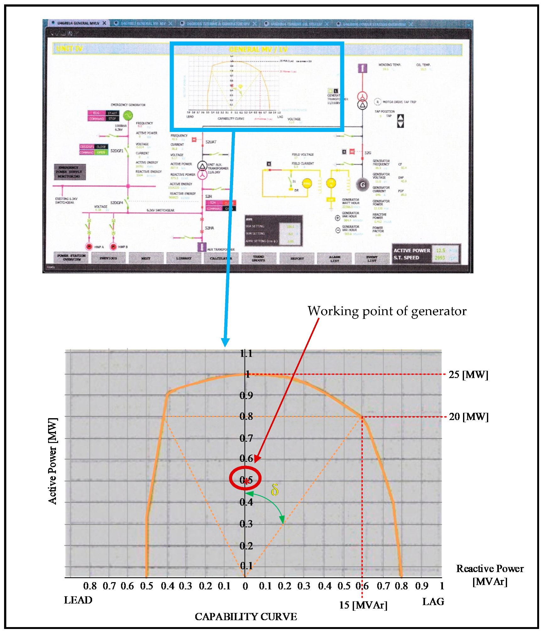
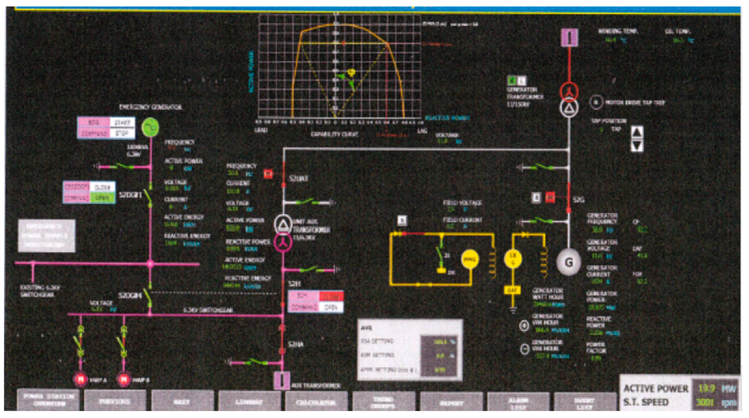
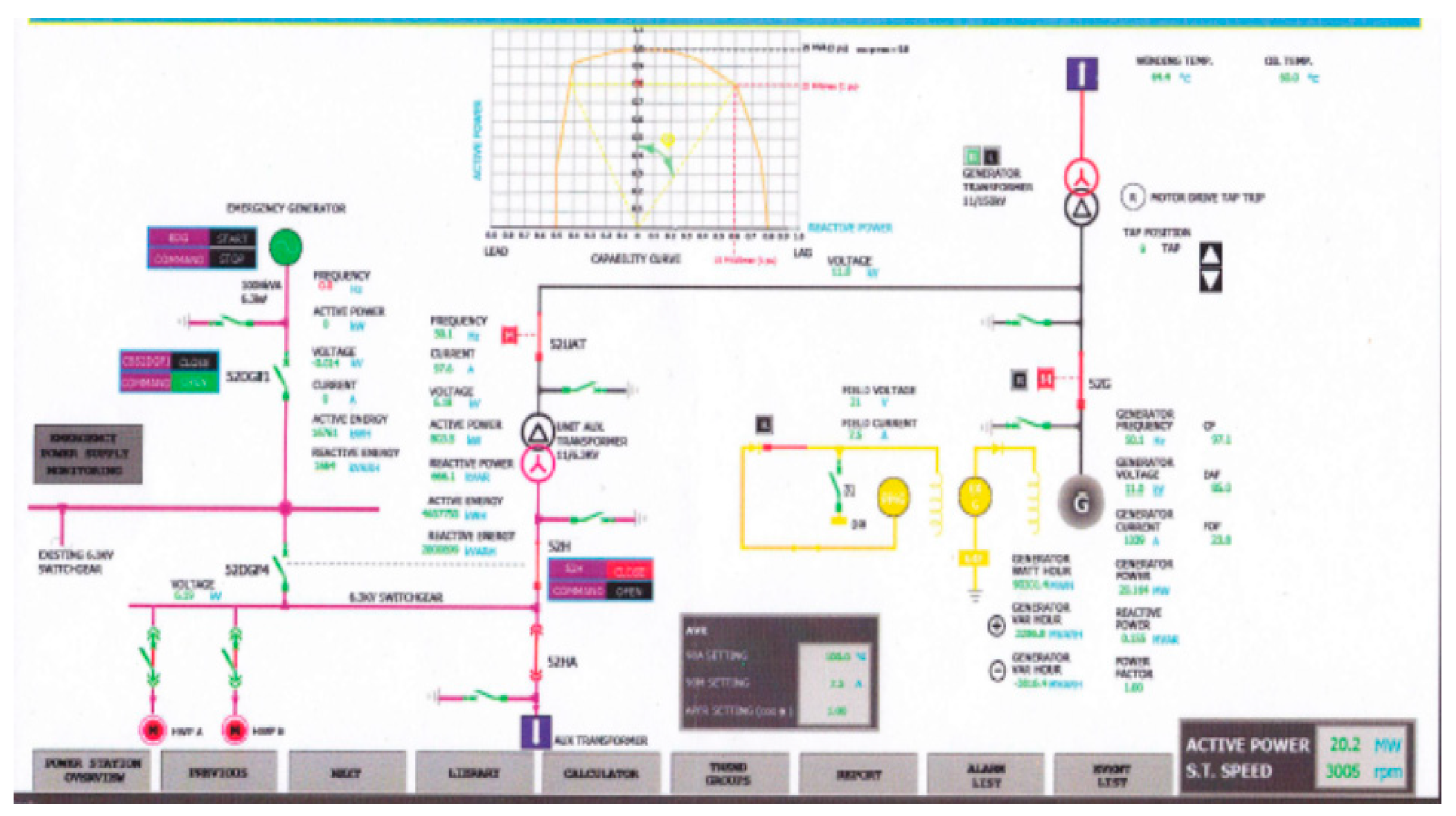
• Developing a virtual visualization of a capability curve simulation to visualize the generator operation conditions. The visualization of GCC is used to monitor the working point of the generator.
• The simulation of the generator capability curve visualization is able to show the various possibilities that occur in the operation of a generator as they happen in reality.

The remainder of this paper is structured as follows. Section 2 describes the generator capability curve. Section 3 presents the proposed method. Section 4 verifies the results of the simulation. Finally, Section 5 concludes the study.

2. Generator Capability Curve

2.1. Devolopment of Generator Capability Curves

A synchronous generator is a type of electric machine that functions to produce an alternating voltage by converting mechanical energy into electrical energy. Mechanical energy is obtained from the rotation of the rotor, which is driven by the prime mover. Meanwhile electrical energy is produced from the electromagnetic induction process that occurs in the stator coil and rotor. The generator operating point limits are stated and visualized in the form of the generator capability curve. The generator load capability curve and generator operating capability include active power (MW), reactive power (MVAr), and apparent power (MVA). The capability curve is drawn on the $PQ$ axis. The capability curve generator is formed based on the phasor diagram, as shown in Figure 1. We assume that the terminal voltage $\left(V_{\mathsf{\varphi }}\right)$ is constant and the stator resistance is negligible. The voltage terminal generator is a phasor reference.

The capability curve generator is formed based on the following steps [18,19]: The phasor diagram from Figure 1 is plotted on the $x$ and $y$ axes, which represent the voltage axis, as shown in Figure 2. In Figure 1a, the generator is in an over-excited condition if $\left|E_{\mathrm{i}}\right|cos\delta >\left|V_{\mathsf{\varphi }}\right|$. Length $\left|E_{\mathrm{i}}\right|cos\delta$ equals line length OB and length $\left|V_{\mathsf{\varphi }}\right|$ equals line length OA. Line OB is longer than line OA, so it can be stated that $\left|E_{\mathrm{i}}\right|cos\delta >\left|V_{\mathsf{\varphi }}\right|$. In the over-excitation condition, the generator work is affected by the field current ($I_{\mathrm{f}}$). In this condition, the generator sends reactive power ($Q$) to the system with a positive power factor angle (pf = positive). Viewed from the system, the generator is like a capacitor.

• The $x$ and $y$-axis of the phasor diagram in Figure 2 are converted into active and reactive power. The $x$-axis becomes the reactive power (MVAr) and the $y$-axis becomes the active power (MW). To change the scale from the voltage unit to the power unit, it is multiplied by $3\frac{V_{\mathsf{\varphi }}^{}}{X_{\mathrm{s}}}$, as shown in Figure 3.
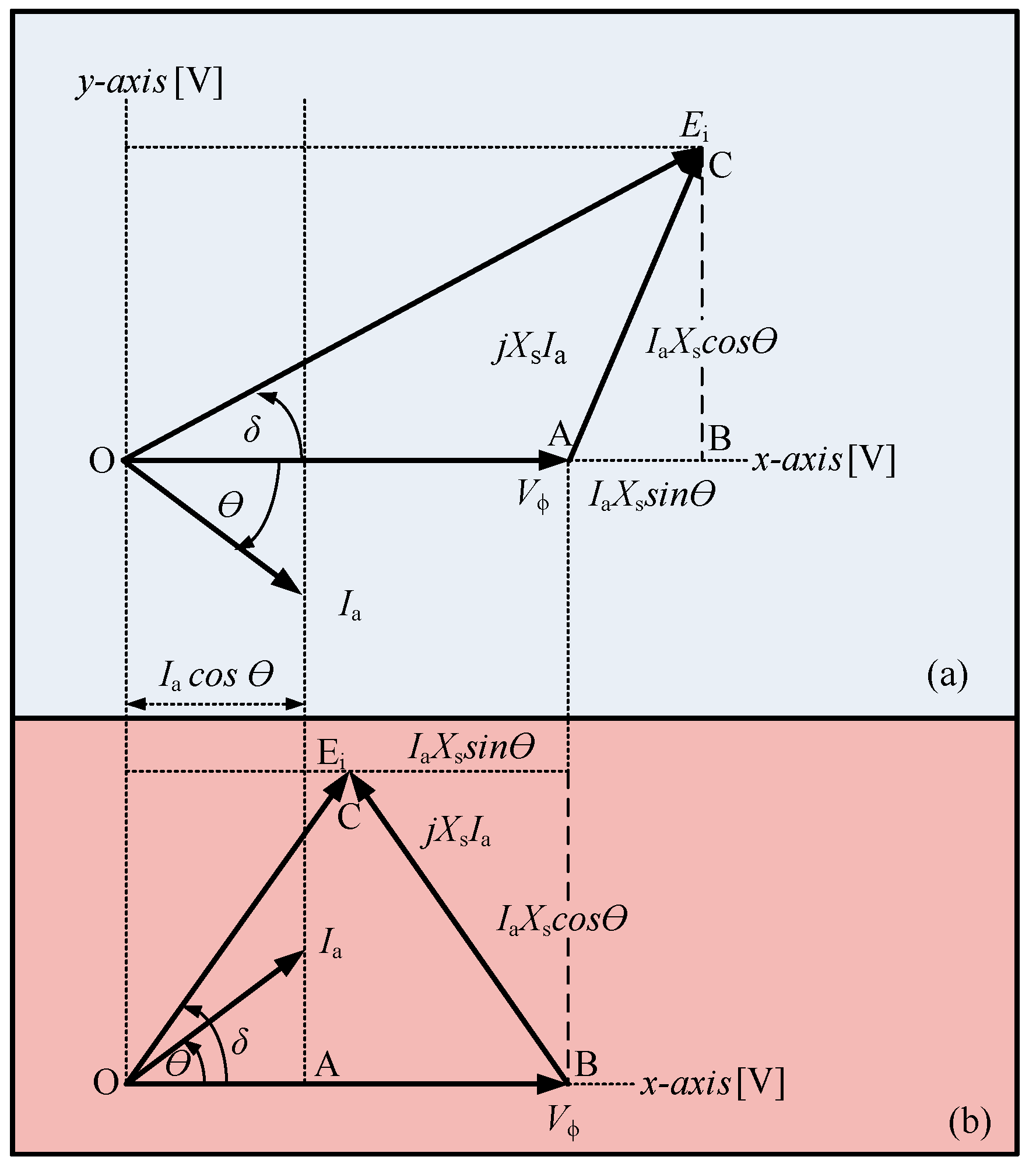
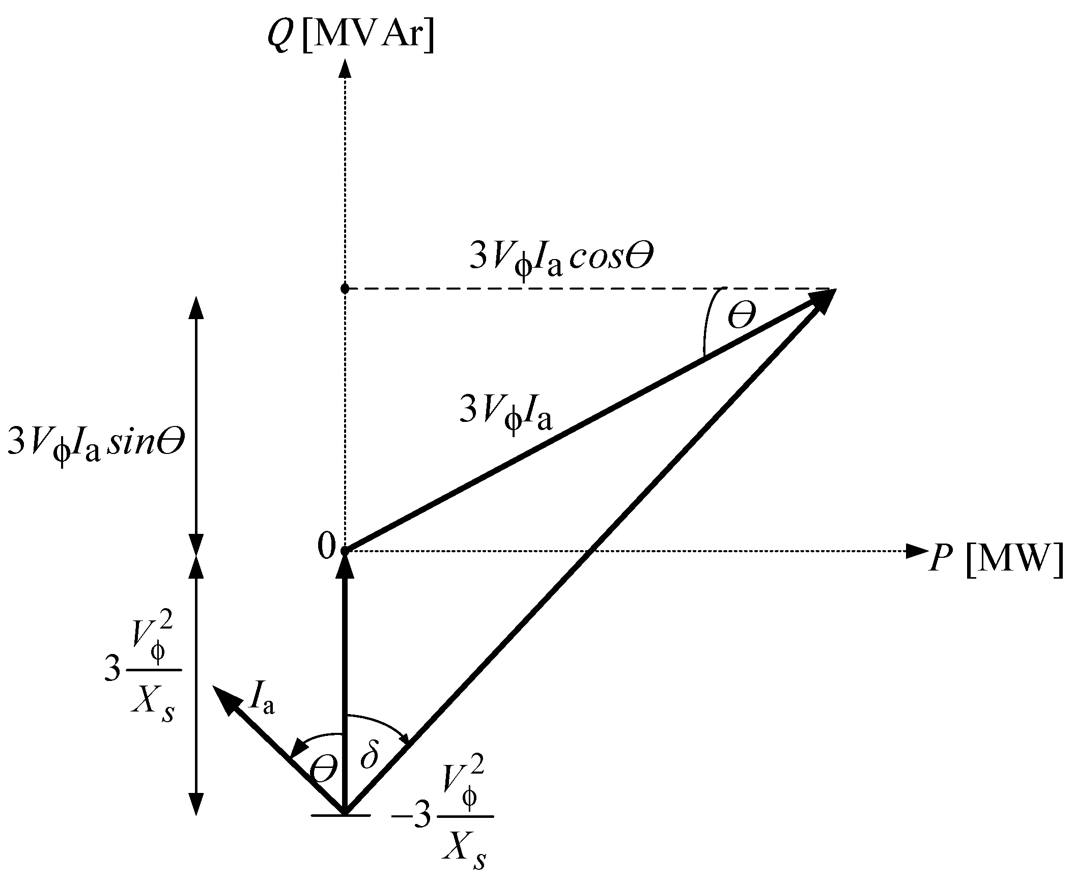
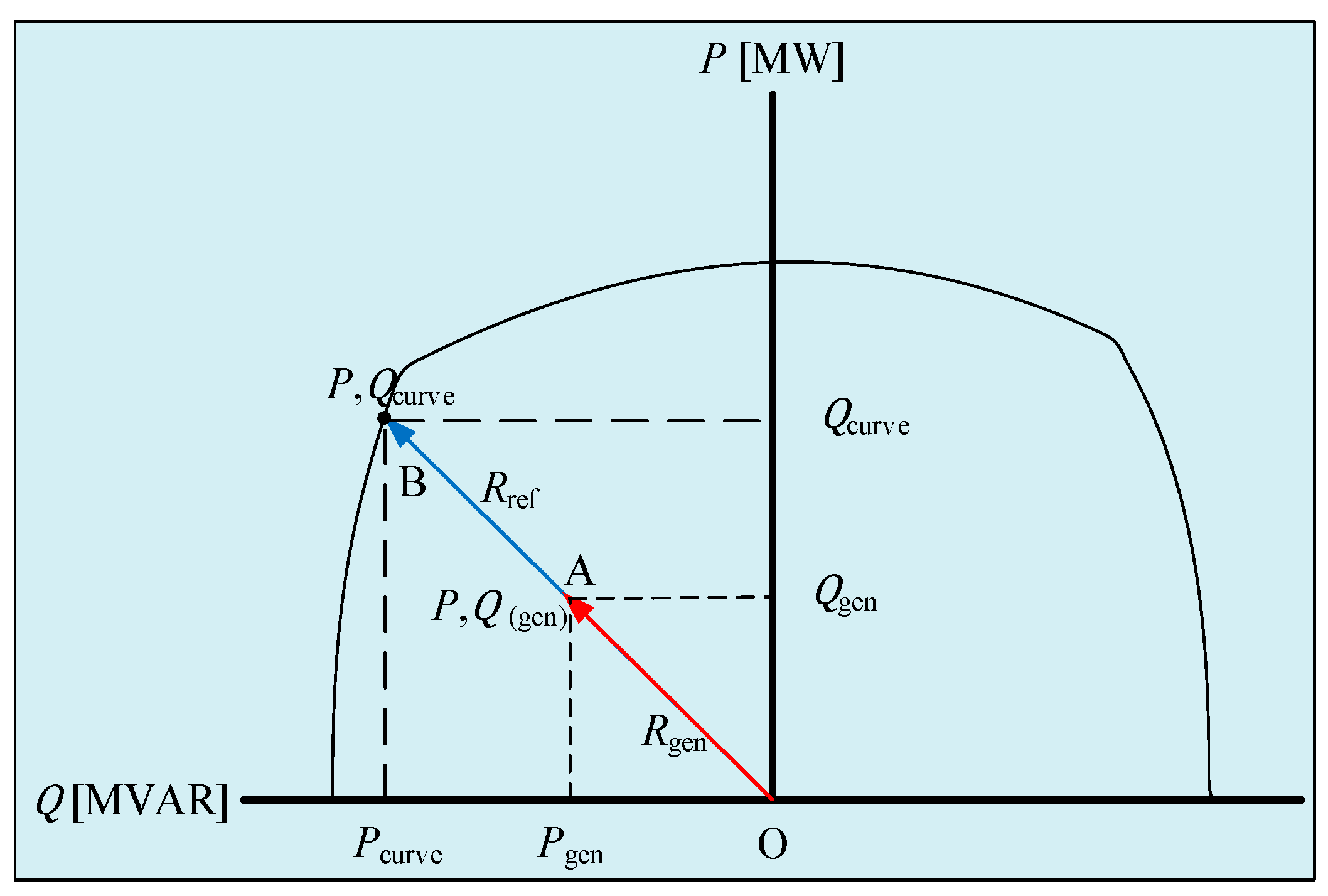
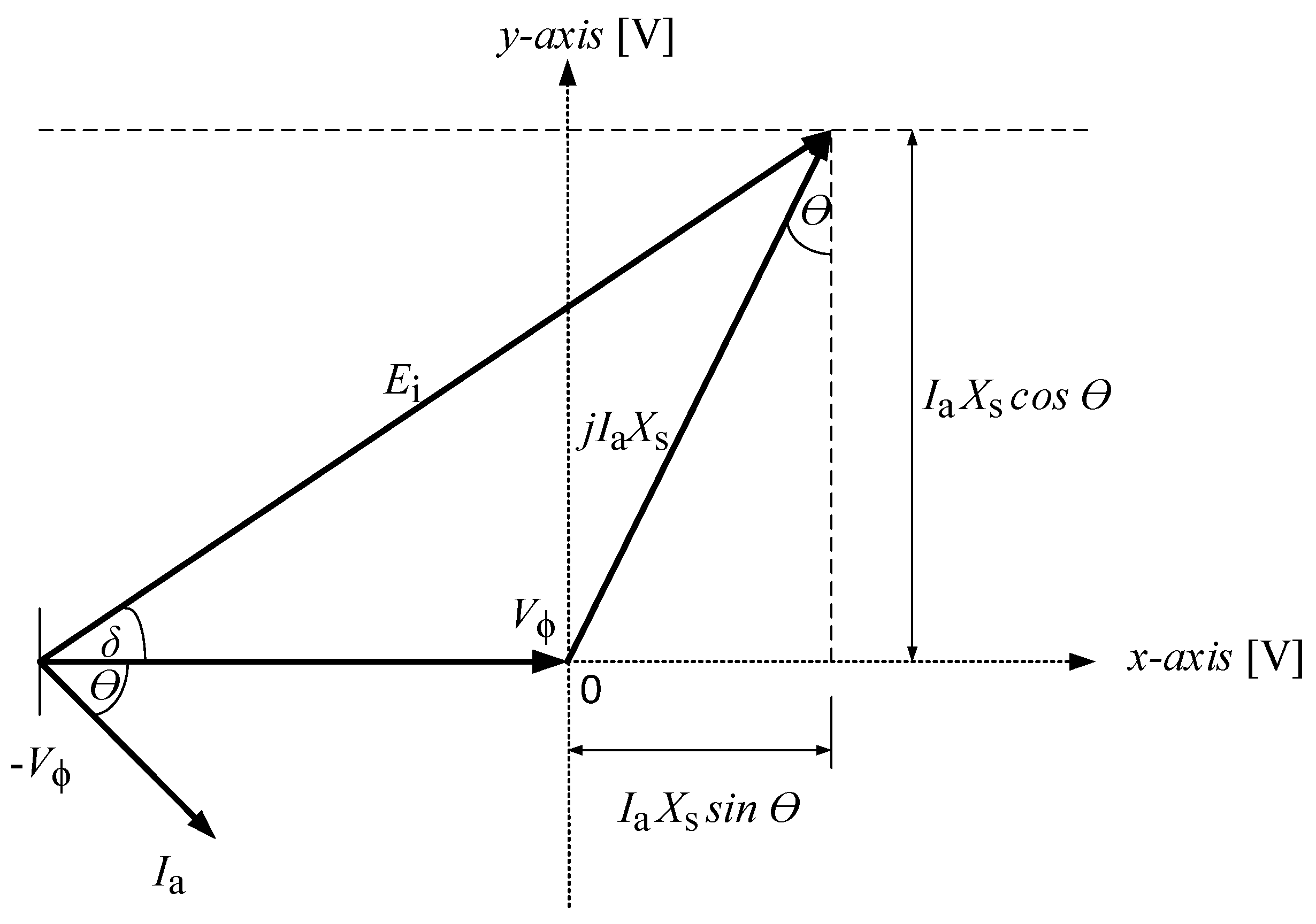
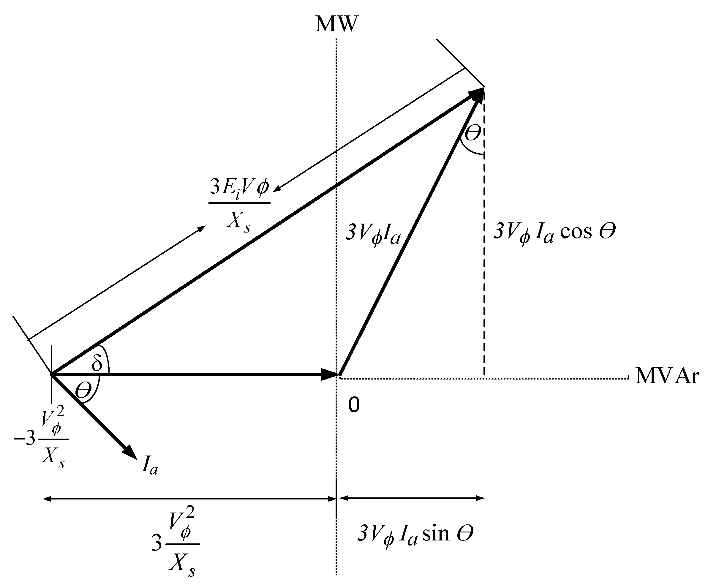
• In theory, the generator capability curve is formed with active power (MW) on the x-axis and reactive power (MVAr) on the y-axis. Therefore, the phasor diagram of Figure 3 is rotated ${90}^{°}$ towards the O-axis counterclockwise, producing a phasor diagram with active power (MW) on the $x$-axis and reactive power (MVAr) on the $y$-axis, as shown in Figure 4.
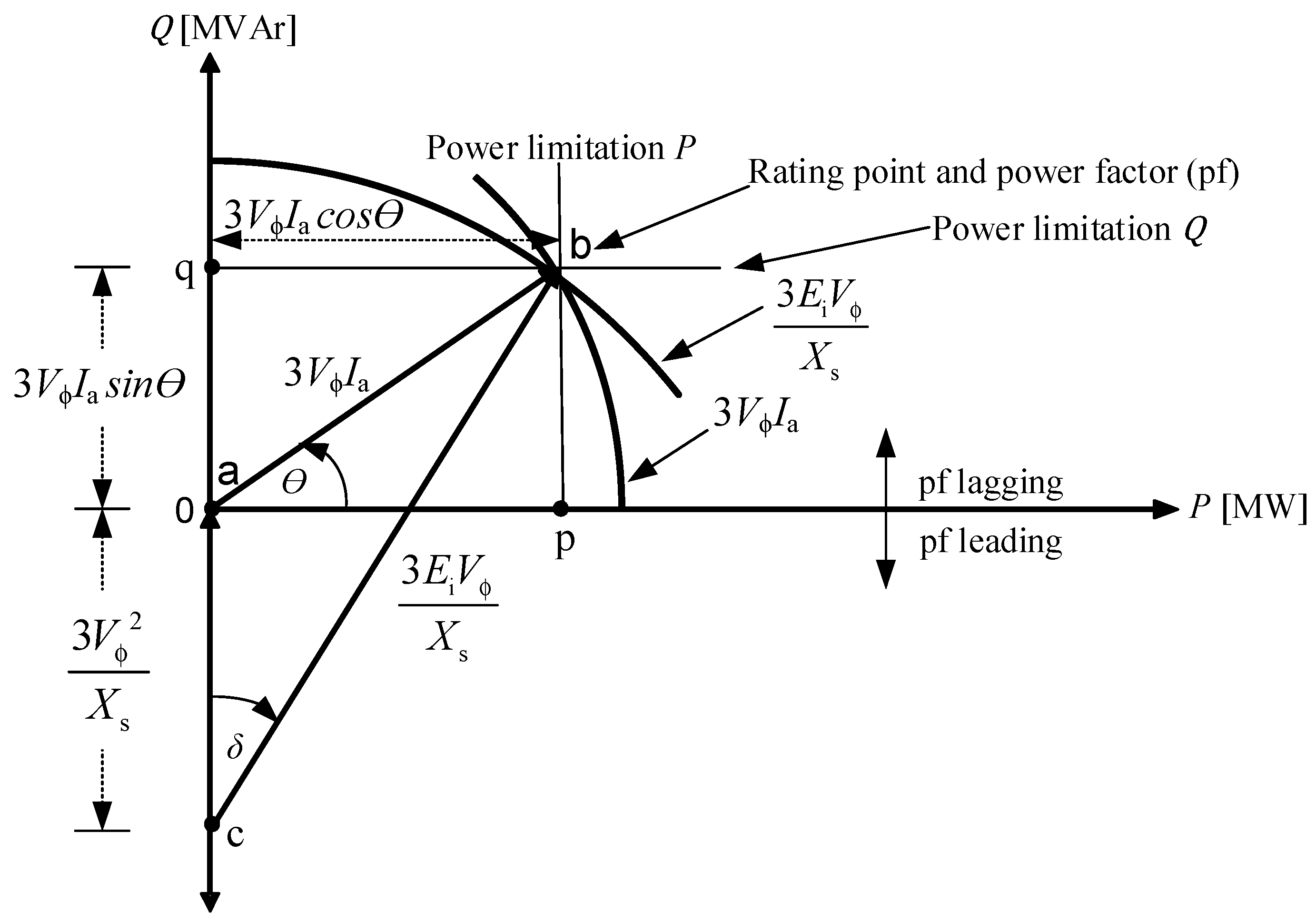
• Based on the power diagram of a synchronous engine, the generator working area is on the positive $x$-axis while the motor work is on the negative $x$-axis. Therefore, the phasor diagram from Figure 4 is mirrored against the $y$-axis, resulting in a phasor diagram in Figure 5 which states the generator working area on the positive $x$-axis.

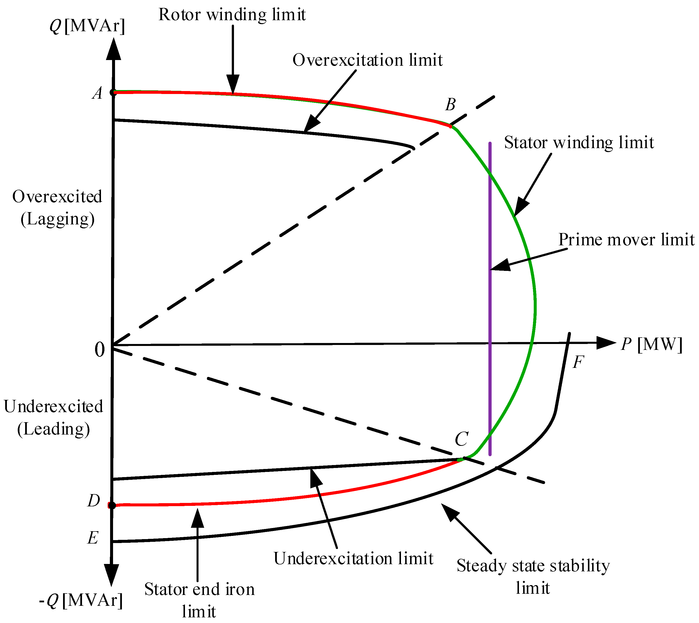
2.2. Generator Operation Limits

Based on the constraints of the operation generator limitations, the capability curve is formed. The limit of the generator operating capability in sending power to the system is illustrated in Figure 6 [20].

where:

• $P$: active power (MW).
• $Q$: reactive power (MVAr).
• $E_{\mathrm{i}}$: apparent power (MVA).
• $I_{\mathrm{a}}$: stator current (A).
• $I_{\mathrm{f}}$: field current (A).
• $X_{\mathrm{s}}$: synchronous reactance (p.u).
• $V_{\mathsf{\varphi }}$: terminal voltage (V).
• 3V_ϕ I_a cos θ: active power limitation (MW).
• 3V_ϕ I_a sin θ: reactive power limitation (MVAr).
• 3V_ϕ I_a: stator current limitation (A).
• $\frac{3E_{\mathrm{i}}{V}_{\mathsf{\varphi }}}{X_{\mathrm{s}}}$: rotor current limitation (A).
• Point b: generator rating (MVA).
• pf: power factor (p.u).

The GCC is limited by some constraints, as follows:

1.

Generator power limit:

The active power (P) of the generator is generated by adjusting the prime mover speed of the generator. The limit for the active power of the generator is stated by:

$$P=3V_{\mathsf{\varphi }}{I}_{\mathrm{a}}cos\theta .$$

(1)

Visually, the active power limit of the generator is shown in Figure 6 by drawing a vertical line from point b to point p, which is parallel to the axis $Q$.

Generator reactive power is generated by adjusting the generator excitation system—namely, the field amplifier current ($I_{\mathrm{f}}$). The limit of the reactive power ($Q$) of the generator is expressed by:

$$Q=3V_{\mathsf{\varphi }}{I}_{\mathrm{a}}sin\theta .$$

(2)

Visually, the reactive power limit of the generator is shown in Figure 6 by drawing a horizontal line from point b to point q, which is parallel to the axis $P$.

The complex power limit or rated power of the generator is expressed by:

$$S=3V_{\mathsf{\varphi }}{I}_{\mathrm{a}},$$

(3)

Visually, the complex power limit of the generator is shown in Figure 6, where point b is the generator rating point (MVA).

Operation in over- and under-excited modes results, as a consequence, in the greater heating of some elements of the generator—i.e., the stator and rotor windings, the end zone of the stator core, etc. During the long-term operation of a generator, in both over- and under-excited modes, some undesirable phenomena can occur, particularly because of the premature aging of the stator and rotor insulation.

2.

Armature current limit:

Armature current ($I_{\mathrm{a}}$) flowing in the stator winding results in power loss ($I^{2}R)$. This power loss can result in an increase in the conductor temperature and that of the nearby environment. If allowed, this temperature increase can occur continuously. Therefore, one of the limitations in generator work is the maximum current that the anchor can carry without exceeding the allowable heating limit. Visually, the stator current limit is shown in Figure 6:

• Depicted as a circle $3V_{\mathsf{\varphi }}{I}_{\mathrm{a}}$
• Center of circle: at point a (0,0);
• Length of radius of circle: length of line a–b, which is the generator rating $3V_{\mathsf{\varphi }}{I}_{\mathrm{a}}$.

3.

Field current limit:

Due to the heating resulting from copper losses in the rotor windings, the rotor currents also determine the limits in generator operation. The rotor current limit is affected by the excitation current. The excitation current can be maintained constant by maintaining the direct current if wrapped in a constant field. Visually, the rotor current limit is shown in Figure 6:

• Depicted as a circle $\frac{3E_{\mathrm{i}}{V}_{\mathsf{\varphi }}}{X_{\mathrm{s}}}$
• Center of circle point: at point c $\left[0,\frac{3{E_{\mathsf{\varphi }}}^2}{X_{\mathrm{s}}}\right]$.

4.

Length of radius of circle: length of line c-b $\frac{3E_{\mathrm{i}}{V}_{\mathsf{\varphi }}}{X_{\mathrm{s}}}$

5.

Stator-end region heating limit.

The heating of the stator core ends determines the operating limits of the generator in the weak excitation region (the area below the $P$-axis). The heating of the stator core ends is caused by the flux leaking in the air gap. The leakage flux is the sum of the load current flux vectors in the stator winding and direct current flux in the rotor winding. Most of the leaking flux passes through the air gap between the stator winding and the rotor, and a small portion of the leaking flux remains at the end of the stator winding. Flux leaks at the end of the stator core occur at the end of the stator core and around it. The leaky flux rotates at a synchronous speed, thus inducing eddy currents throughout the stator structure joints and also the rotor. Eddy currents can be reduced because the stator core structure is made of a magnetic steel thin layer perpendicular to the rotor axis, with each layer isolated from the other layers. The magnetic steel film effectively reduces the eddy currents when alternating current is applied in parallel to the coating. The stator-end region heating limit is depicted as a circle C,D in Figure 7.

6.

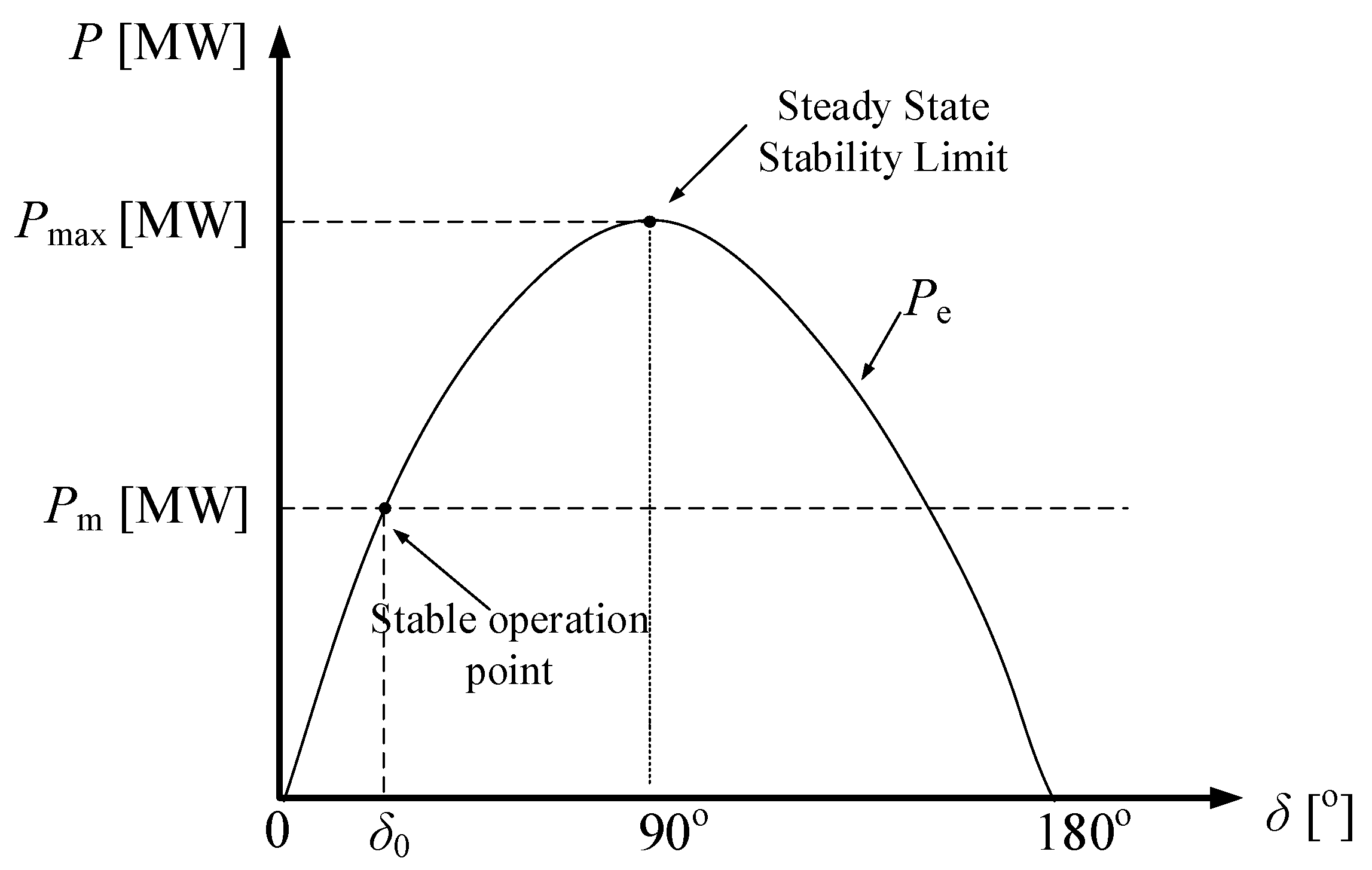
Steady-state stability limit.

Another limit in the distribution of power by the generating unit is the steady-state stability. When operating at full load, generators tend to work in the leading region, which is the area that absorbs reactive power from the system. In this condition, the generator must be operated carefully so that the steady-state stability limit is added in the generator operating area. In this condition, the generator power angle, which is the angle between the stator and the rotor, will be close to the steady-state stability point of the generator operation. If this condition is allowed and the power continues to increase uncontrollably, there will be instability of generator operation or the generator will experience a loss of synchronization. With the loss of synchronization, the rotor and stator flux speeds become different, and this results in a vibration torque, which creates the potential for induced currents to occur in the rotor structure. In this condition, the generator must be turned off immediately.

Steady-state operating conditions are achieved when the mechanical output power ($P_{\mathrm{m}}$) is balanced with the electrical output power ($P_{\mathrm{e}}$). The relationship between $P_{\mathrm{m}}$ and $P_{\mathrm{e}}$ is shown in Figure 8, where the horizontal line is the mechanical output power generated by the starting generator. If the load on the generator increases, the rotor will slow down, and, vice versa, it will be faster if the load decreases. Under normal conditions, the change in the rotor angle will slightly “overshoot”—that is, it will be a little slower or faster.

• If $P_{\mathrm{e}}$ > $P_{\mathrm{m}}$ or $\delta$ > ${\delta }_0$, the rotor is decelerating;
• If $P_{\mathrm{e}}$ = $P_{\mathrm{m}}$ or $\delta$ = ${\delta }_0$, stable operation point;
• If $P_{\mathrm{e}}$ < $P_{\mathrm{m}}$ or $\delta$ < ${\delta }_0$, the rotor is accelerating.

Here,

• $\delta$ is the power angle between voltage $E_{\mathrm{i}}$ and $V_{\mathsf{\varphi }}$ (engine torque angle);
• $P_{\mathrm{m}}$ is the mechanical output power (MW);
• $P_{\mathrm{e}}$ is the electrical output power generator (MW).

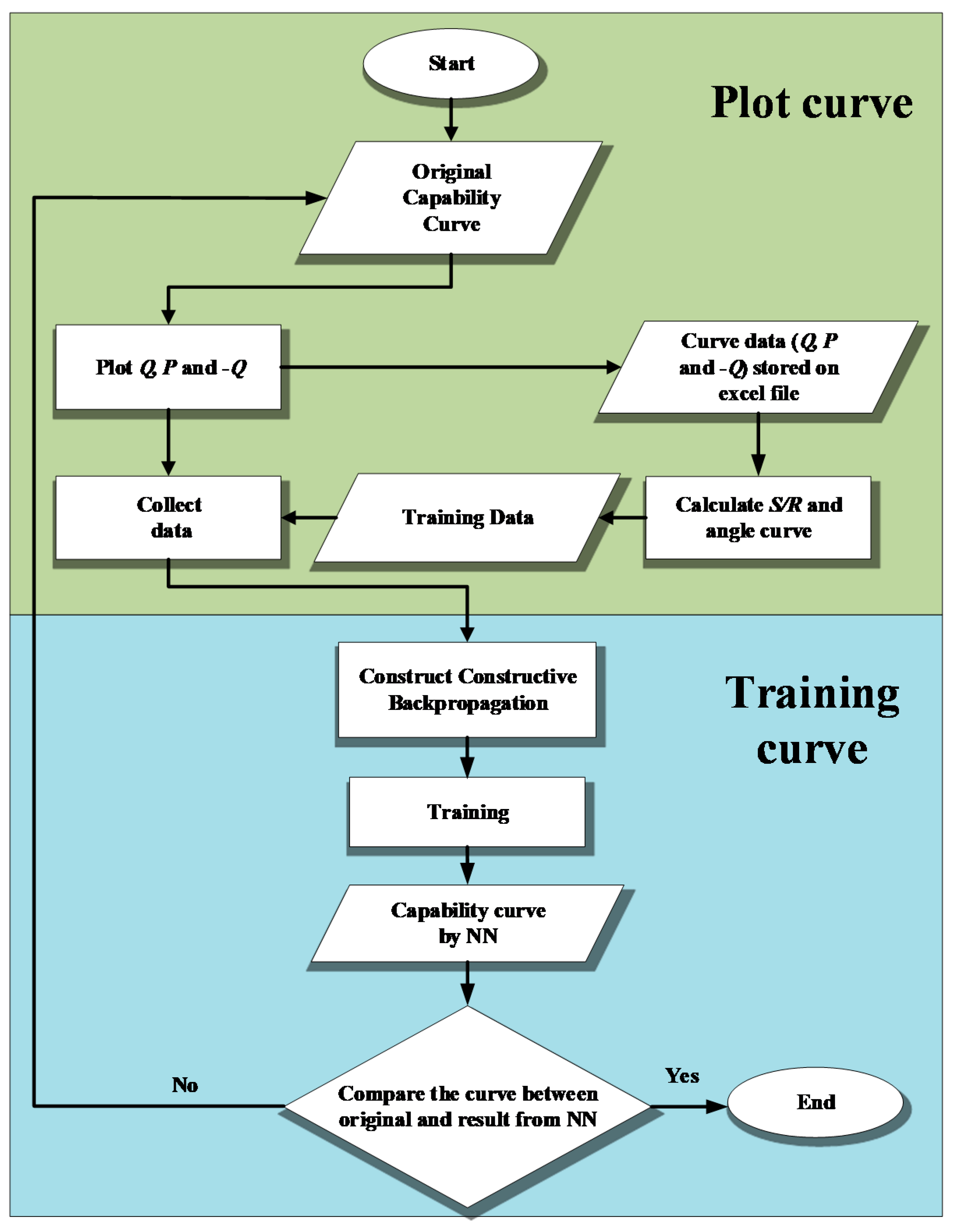
The maximum generator power delivered to the system based on the power angle curve in Figure 8 is stated as follows:

$$P_{\mathrm{e}}=\frac{3E_{\mathrm{i}}{V}_{\mathsf{\varphi }}}{X_{\mathrm{s}}} sin\delta .$$

(4)

Equation (4) is the stability limit when $\delta$ = ${90}^{°}$. The maximum power that can be supplied by the generator occurs when $\delta$ = ${90}^{°}$.

3. Proposed Method

The neural network model with the constructive backpropagation method is used to construct the generator capability curve. The formation of the capability curve is divided into two stages: the first is plotting the capability curve to obtain $P$ and $Q$ points, and second is training for the curve data. The flow chart of the generator capability curve formation is shown in Figure 9.

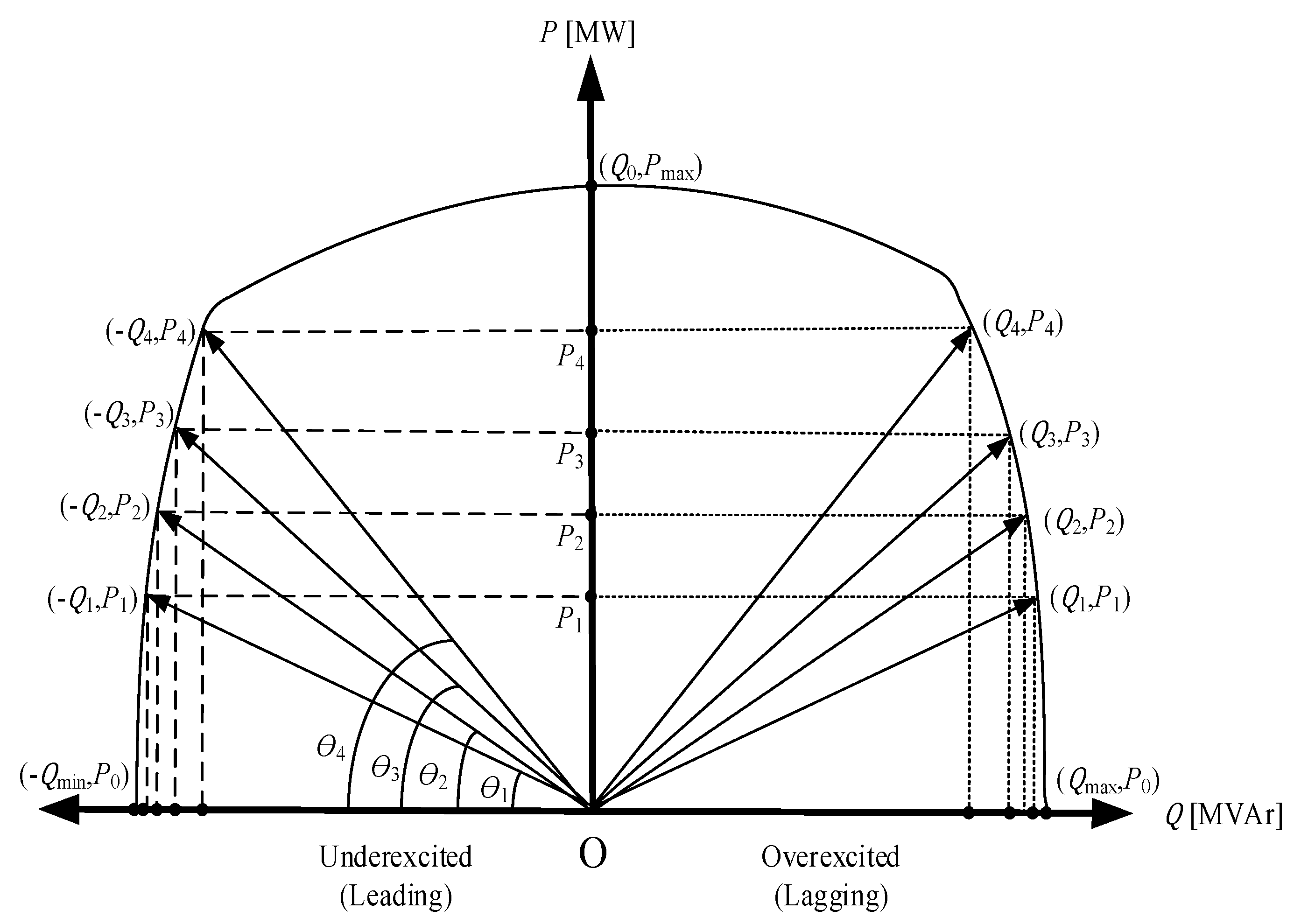
3.1. Plot the Original Capability Curve

A capability curve plot is made to obtain $P$ and $Q$ data pairs from the capability curve. How to plot the generator capability curve is shown in Figure 10 with three steps of line drawing; the first is drawing a line from point $\mathrm{O}$ to reach the boundary of the curve line. Then, from the end of the line pull (the point at the curve line), the next line is drawn, with the first one in the direction of the x-axis so that the length of $Q$ is obtained and the second one along the y-axis to obtain the length $P$—that is, from the $Q_{\min }$ limit to the curve $Q_{\max }$ limit so that as many $P$ and $Q$ data pairs as possible are obtained. In this case, 81 data pairs are generated, consisting of $P$ and $-Q$ data pairs for the leading region and $P$ and $Q$ data pairs for the lagging region.

where

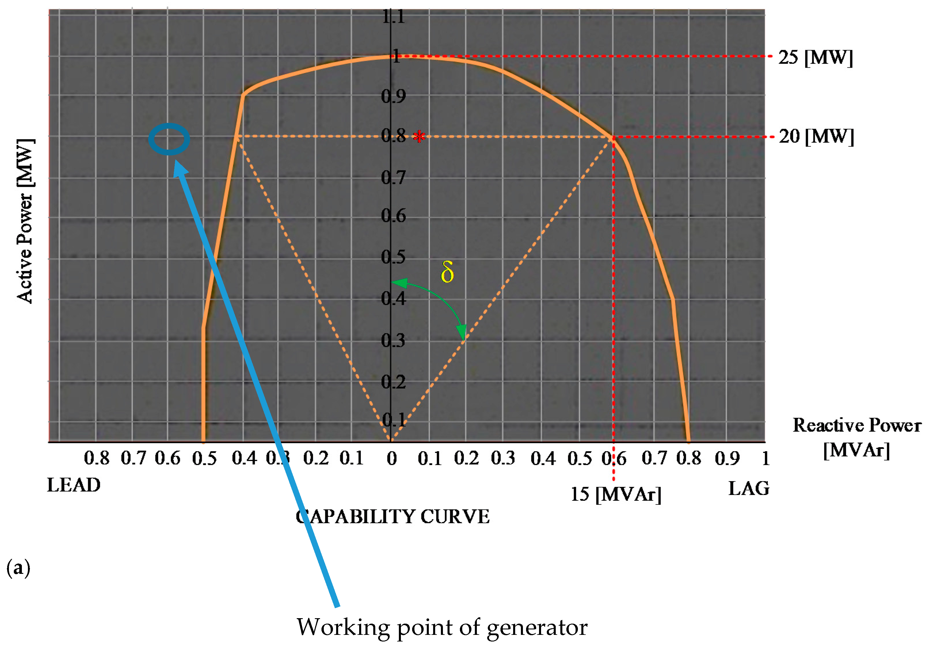
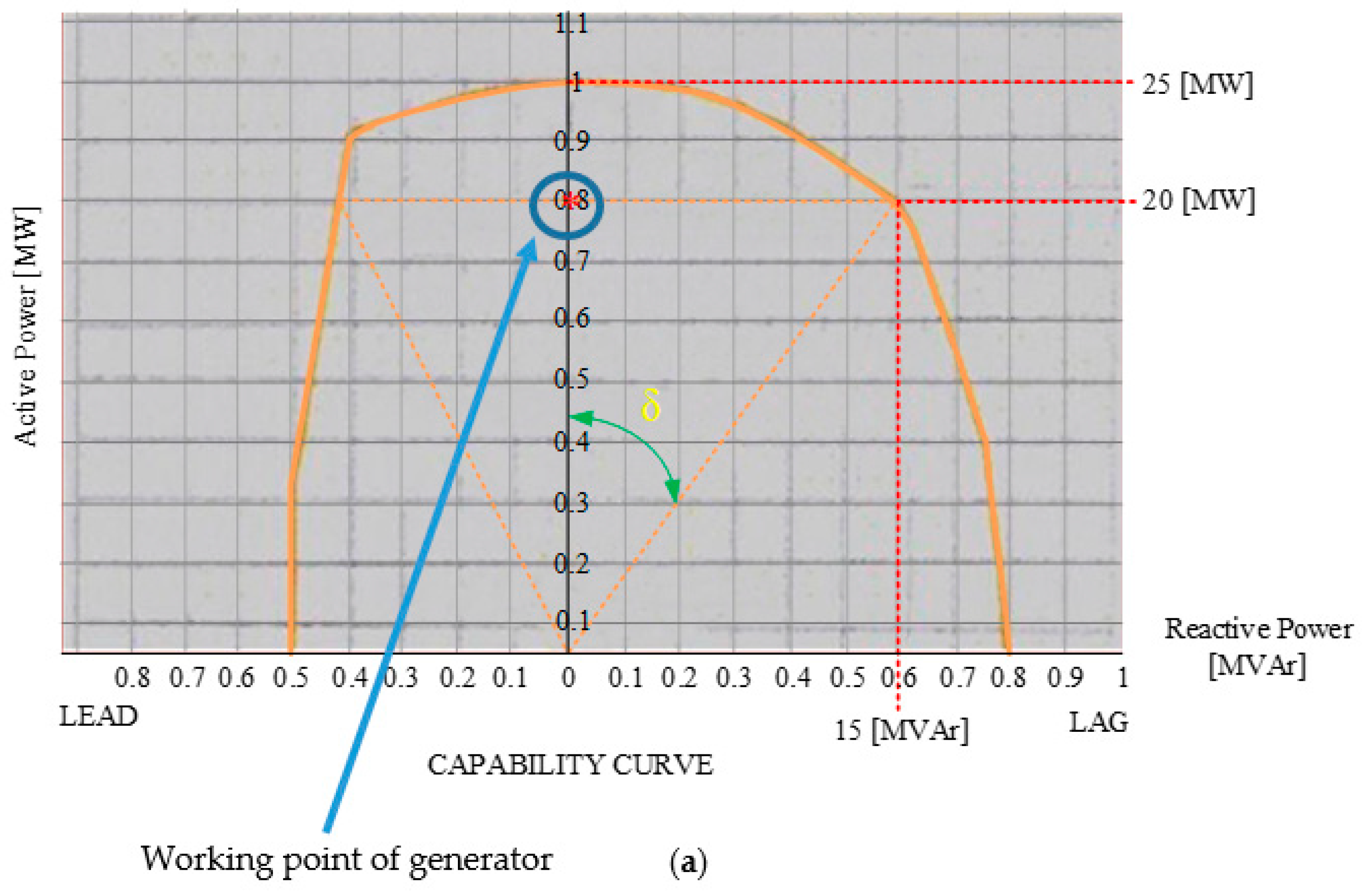
• $Q_{\max }$: maximum reactive power point (in overexcited condition/lagging area);
• $P_0$: the power point is active when $P$ = 0;
• $Q_{\min }$: minimum reactive power point (in underexcited/leading area);
• $Q_0$: the point of reactive power when $Q$ = 0.

3.2. Training the Curve Data

To obtain a capability curve by neural network (NN) similar to the original capability curve of the generator, training on the $PQ$ curve data is required. Curve data training uses the neural network with the constructive backprogation (CBP) method. The process of forming the construction of adding hidden units for the constructive backropagation learning method occurs bit by bit.

In this paper, the training stages are carried out as follows:

• Load data: the $PQ$ data resulting from the generator capability curve plot is stored in Microsoft Excel, then is called using the Matlab program.
• When calculating the complex power and angle $\theta$ curve, the calculation is conducted with the Matlab program:

  $$S_{\mathrm{curve}}=\sqrt{P^2+Q^2},$$

  (5)

  $${\theta }_{\mathrm{curve}}=ta{n}^{-1}\frac{Q}{P}.$$

  (6)

Enter the input and target data.

Input: angle $\theta$ curve.

Target: complex power curve ($S$) or the distance between the center point and curve line (R).

4.

Construct the hidden unit layer.

The construction of the addition of hidden screens with the constructive backprogation training method is carried out one by one from the smallest number until a hidden screen is obtained with a small error rate.

5.

Build a constructive backpropagation network.

The curve training process using the constructive backprogation method begins with the weight initialization process followed by the feedforward stage, which is shown in the use of the “newff” component as a function that will create a feedforward network that adds weighted input signals to the hidden layer and the output layer. The constructive backropagation training algorithm is as follows:

• Initialization—namely, the initial formation of ANN in the form of ANN without hidden units. The weight of the initial configuration is calculated by minimizing the sum of squared error (SSE). Weights that have been found are fixed.
• New hidden unit training to connect the input to the new unit and connect the output to the output unit. All the weights connected to the new unit are adjusted by minimizing the SSE (modified SSE).
• Freezing of new hidden units—namely, permanently assigning weights to interconnect with new units.
• Convergence test—that is, if the number of hidden units has produced a viable solution, then the training is stopped. If not, go back to step 2.
• Determine training parameters.

There are several training parameters that are set before the training is carried out—namely, by giving the desired values to these parameters to obtain optimal results. The parameters are listed as follows:

• net.trainParam.show: used to display the change frequency of mse (mean square error).
• net.trainParam.lr: used to determine the rate of understanding (α = learning rate).
• net.trainParam.epochs: used to determine the maximum number of epochs of training.
• net.trainParam.goal: used to specify the mse value limit to stop iteration. The iteration will stop if the mse < limit specified in “net.trainParam.goal”.

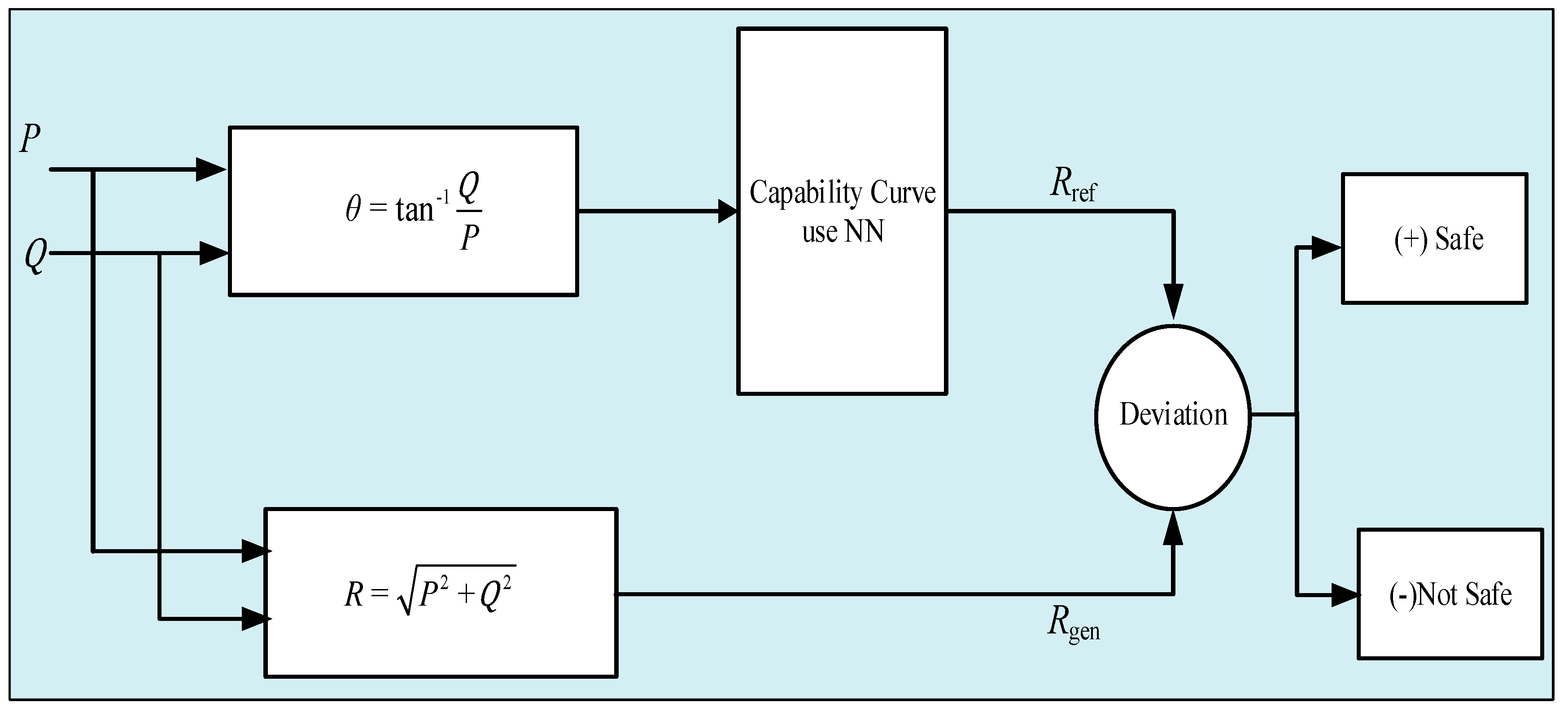
Testing of the generator capability curve from the NN training is carried out to test the safety of the generator. The algorithm for testing the generator capability curve of the NN training results is as follows:

• Entering the active power ($P$) and reactive power ($Q$) of the original capability curve as an input to the capability curve of the NN training results.
• From the $P$ and $Q$ data of the original capability curve, the $\theta$ value and the magnitude of the $R_{\mathrm{gen}}$ are calculated (the power of the generator complex or the radius of the load curve).
• By entering the angle data $\theta$ as an input to the NN yield curve that has been previously generated, the output of the NN yield capability curve will be obtained in the form of $R_{\mathrm{ref}}$ (the radius of the NN yield curve).
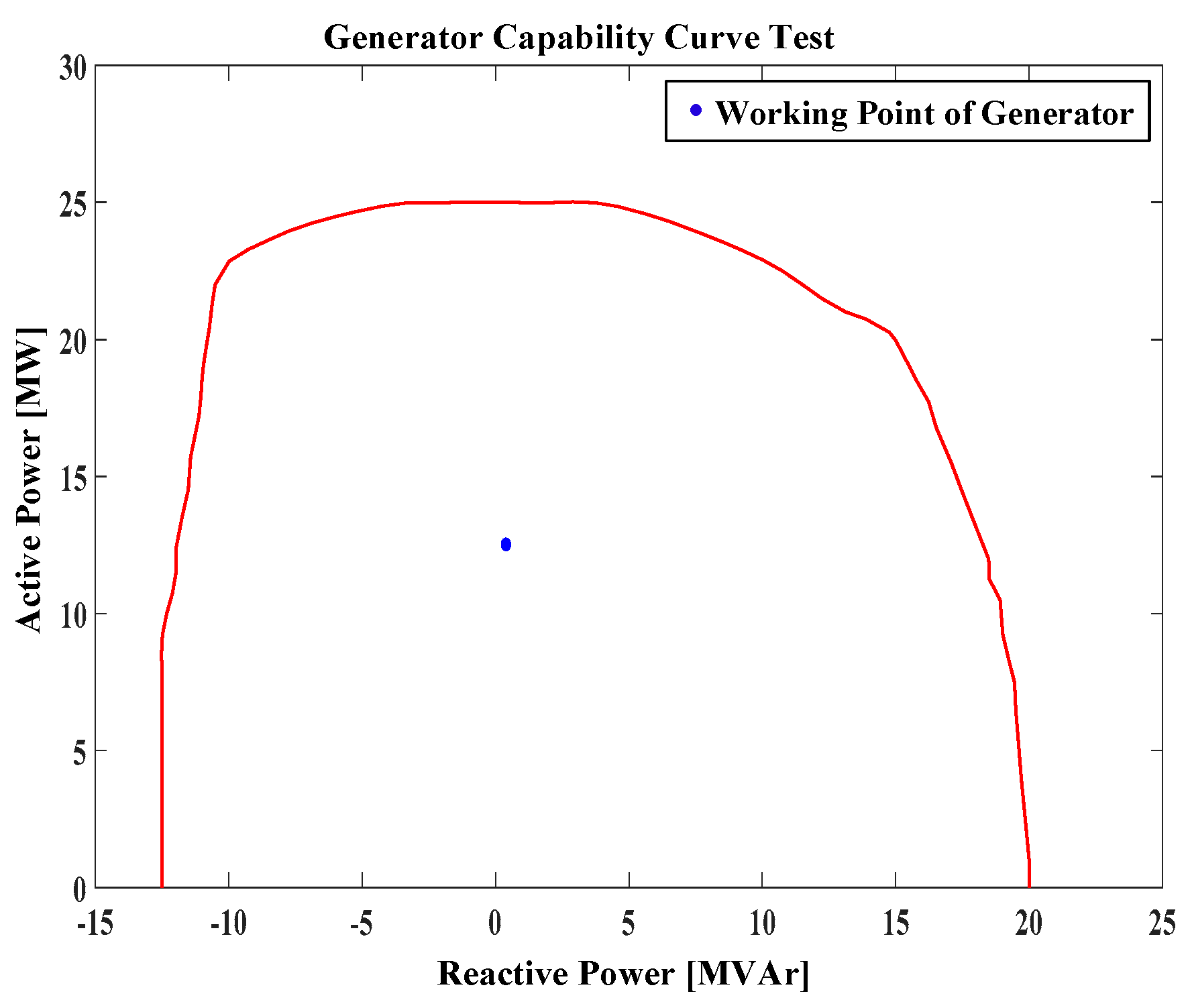
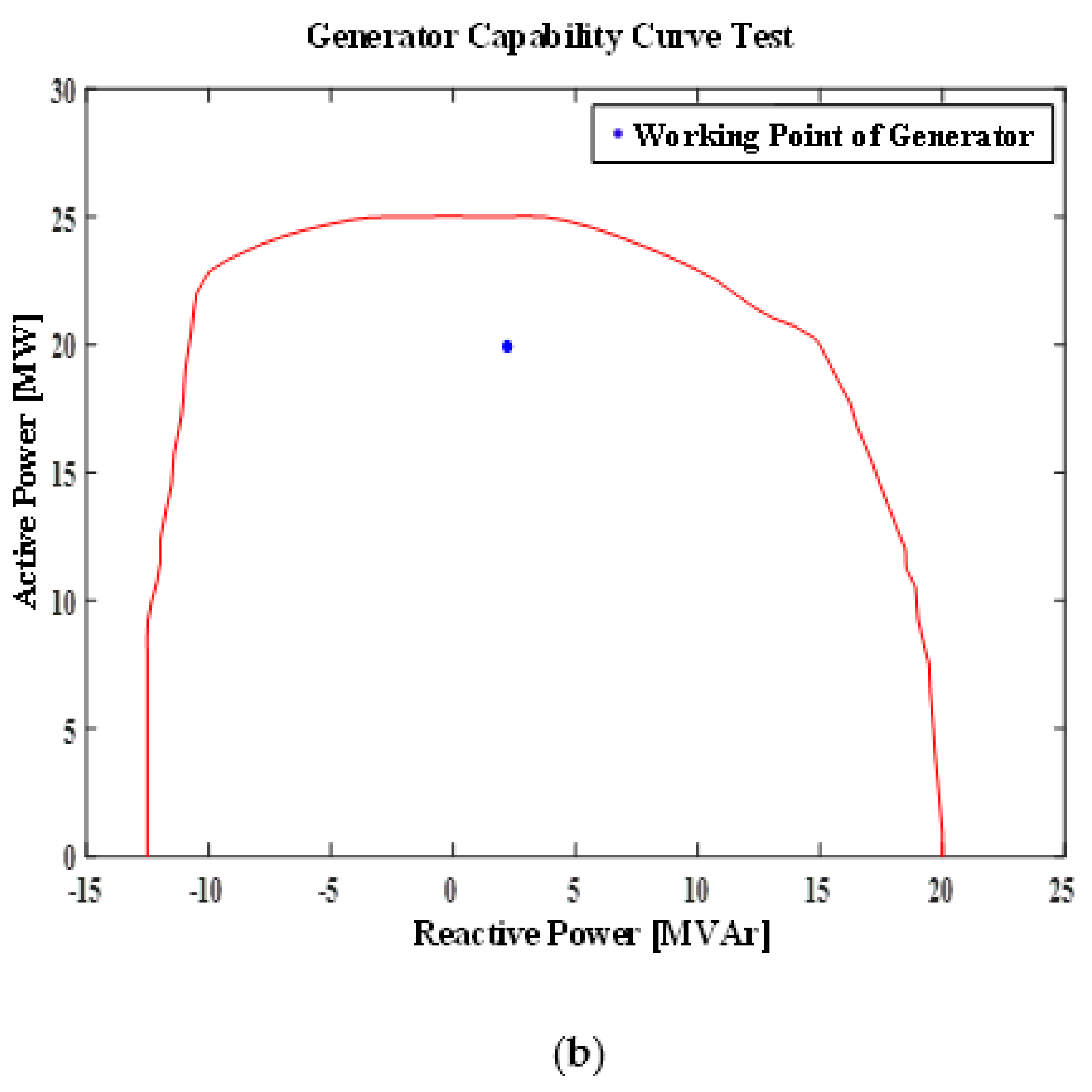
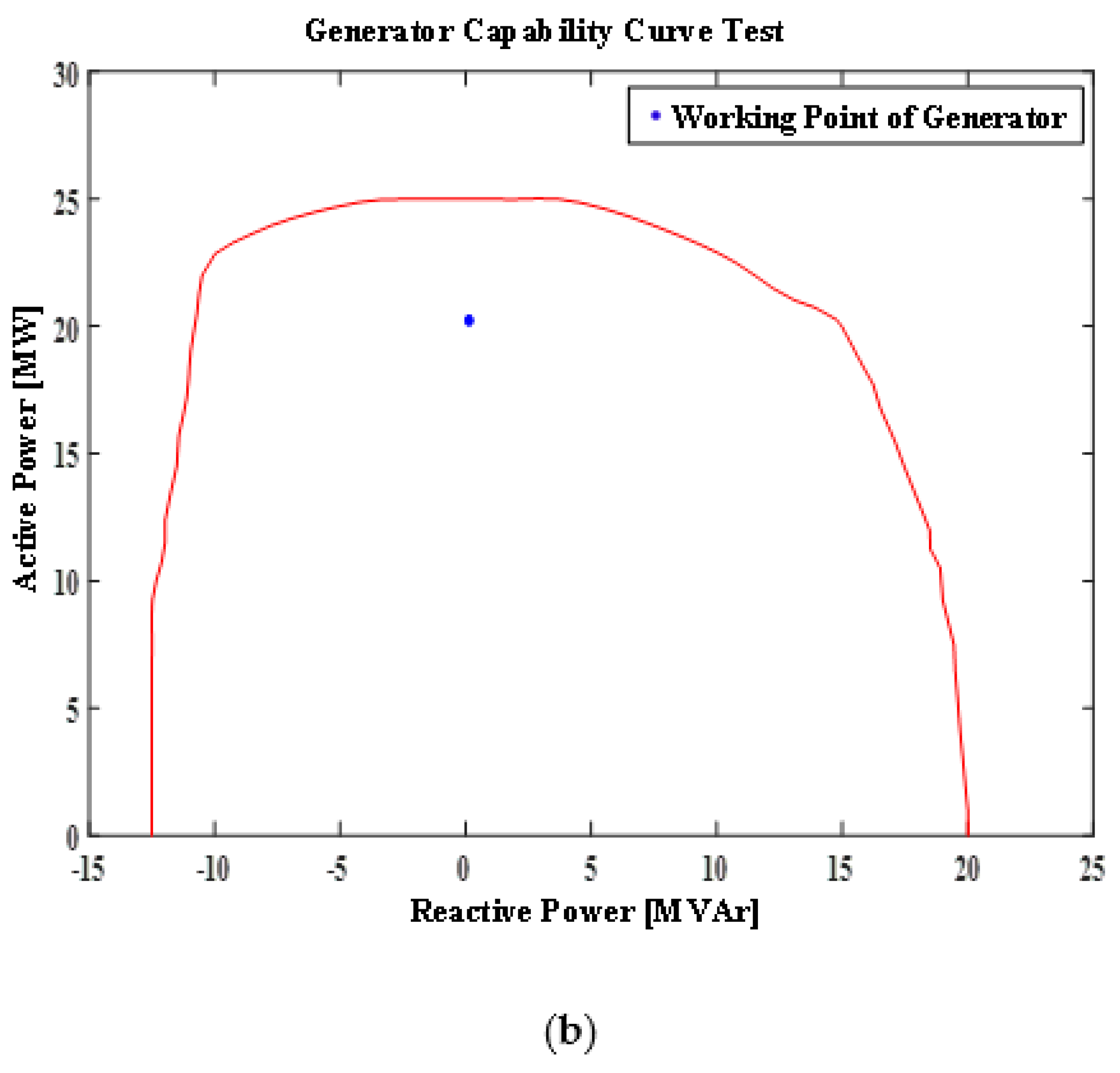
• Generator safety testing is carried out by comparing the $R_{\mathrm{gen}}$ and $R_{\mathrm{ref}}$ values. If $R_{\mathrm{gen}}$ ≤ $R_{\mathrm{ref}}$ and the difference between $R_{\mathrm{gen}}$ and $R_{\mathrm{ref}}$ (difference R) is positive, the generator status is safe. Otherwise, if $R_{\mathrm{gen}}$> $R_{\mathrm{ref}}$ and the difference between $R_{\mathrm{gen}}$ and $R_{\mathrm{ref}}$ (difference $R$) is negative, the generator status is not safe.

Figure 11 shows the relationship between the generator operating point ($P$, $Q$), angle $\theta$, $R_{\mathrm{gen}},$ and $R_{\mathrm{ref}}$. When line OA is the length of the radius of the load ($R_{\mathrm{gen}}$), line OB is the length of the radius of the curve ($R_{\mathrm{ref}}$) and line AB is the difference between $R_{\mathrm{gen}}$ and $R_{\mathrm{ref}}$.

The algorithm for testing the generator capability curve is shown in Figure 12.

4. Results of the Simulation

4.1. Case Study 1

To apply the proposed method, an original capability curve from the generator in Lahendong IV geothermal power plant is used. Lahendong IV geothermal power plant is located in Minahasa, North Sulawesi, Indonesia. Lahendong IV geothermal power plant has a unit generator with a capacity of 20 MW. The specification of the generator is shown in

Table 2. Generator specification.

Generator Name	LH4
Type	GTLRI494/45–2
Output [MVA]	25
Output [MW]	20
Voltage [kV]	11
Current [A]	1312
Excitation voltage [V]	160
Excitation current [A]	808
Phase	3
Power factor	0.8
Frequency [Hz]	50
Number of Poles	2
Speed [rpm]	3000
Production year	2010
Producer	Fuji Electric

.

The original capability curve from the generator in Lahendong IV geothermal power plant is shown in Figure 13. The sign inside the red circle is the working point of the generator, which visualizes that the generator is operated at that condition related to the $P$ and $Q$ of the generator.

The plot of the original capability curve of the Lahendong IV geothermal power plant generator produces a pair of $PQ$ data points shown in

Table 3. The $PQ$ curve data plot.

No.	Pcurve	Qcurve	S	θ	No.	Pcurve	Qcurve	S	θ
1	0.000	20.000	20.000	1.571	41	25.000	0.000	25.000	0.000
2	0.950	20.000	20.023	1.523	42	25.000	−0.750	25.011	−0.030
3	2.000	19.900	20.000	1.471	43	25.000	−1.600	25.051	−0.064
4	3.000	19.800	20.026	1.420	44	25.000	−2.500	25.125	−0.100
5	4.000	19.700	20.102	1.370	45	24.950	−3.400	25.181	−0.135
6	5.250	19.600	20.291	1.309	46	24.900	−4.250	25.260	−0.169
7	6.450	19.500	20.539	1.251	47	24.600	−5.250	25.154	−0.210
8	7.500	19.450	20.846	1.203	48	24.500	−6.000	25.224	−0.240
9	8.250	19.250	20.943	1.166	49	24.250	−6.900	25.213	−0.277
10	9.250	19.000	21.132	1.118	50	24.000	−7.750	25.220	−0.312
11	10.500	18.900	21.621	1.064	51	23.600	−8.500	25.084	−0.346
12	11.250	18.500	21.652	1.024	52	23.250	−9.250	25.022	−0.379
13	12.000	18.500	22.009	0.994	53	22.900	−10.000	24.988	−0.412
14	12.500	18.250	22.120	0.970	54	22.000	−10.500	24.377	−0.445
15	13.450	17.900	22.390	0.926	55	21.250	−10.600	23.747	−0.463
16	14.500	17.450	22.688	0.877	56	20.500	−10.750	23.148	−0.483
17	15.500	17.100	23.079	0.834	57	19.800	−10.800	22.554	−0.499
18	16.750	16.500	23.512	0.778	58	19.050	−10.950	21.973	−0.522
19	17.750	16.250	24.065	0.741	59	18.400	−11.000	21.437	−0.539
20	18.500	15.750	24.296	0.705	60	18.000	−11.050	21.121	−0.551
21	19.500	15.250	24.755	0.664	61	17.200	−11.100	20.471	−0.573
22	20.000	15.000	25.000	0.644	62	16.400	−11.250	19.888	−0.601
23	20.250	14.750	25.052	0.630	63	15.750	−11.450	19.472	−0.629
24	20.750	13.900	24.975	0.590	64	14.500	−11.500	18.507	−0.671
25	21.000	13.100	24.751	0.558	65	13.500	−11.750	17.897	−0.716
26	21.500	12.250	24.745	0.518	66	12.400	−11.950	17.221	−0.767
27	22.000	11.500	24.824	0.482	67	11.500	−12.000	16.621	−0.807
28	22.500	10.750	24.936	0.446	68	10.750	−12.100	16.186	−0.844
29	22.900	10.000	24.988	0.412	69	10.000	−12.300	15.852	−0.888
30	23.250	9.250	25.022	0.379	70	9.250	−12.500	15.550	−0.934
31	23.500	8.500	24.990	0.347	71	8.500	−12.500	15.116	−0.974
32	23.900	7.750	25.125	0.314	72	7.750	−12.500	14.708	−1.016
33	24.100	7.250	25.167	0.292	73	7.000	−12.500	14.327	−1.060
34	24.300	6.500	25.154	0.261	74	6.300	−12.500	13.998	−1.104
35	24.500	5.600	25.132	0.225	75	5.500	−12.500	13.657	−1.156
36	24.900	4.600	25.321	0.183	76	4.650	−12.500	13.337	−1.215
37	25.000	3.750	25.280	0.149	77	3.750	−12.500	13.050	−1.279
38	25.000	2.900	25.168	0.115	78	3.000	−12.500	12.855	−1.335
39	25.000	1.900	25.072	0.076	79	2.000	−12.500	12.659	−1.412
40	25.000	0.750	25.011	0.030	80	1.000	−12.500	12.540	−1.491
					81	0.000	−12.500	12.500	−1.571

, consisting of:

• $P$ point: 81 points;
• $Q$ point: 81 points.

The simulated capability curve display with the original $PQ$ curve data of the generator in the Lahendong IV geothermal power plant is shown in Figure 14.

The capability curve from the NN training results already recognizes the target as the initial capability curve, which are the $PQ$ curve data. It is proven that the capability curve of the NN training results (red line) is similar to the $PQ$ curve data target (blue line). A trial of the capability curve of the NN training results was carried out to obtain the work point of the generator so that it could be determined whether the generator worked at safe limits or not. The generator work point is declared safe if it meets the requirements of $R_{\mathrm{gen}}$ ≤ $R_{\mathrm{ref}}$. The testing of the generator capability curve is carried out on several loading conditions—namely, by entering the $P$ and $Q$ values as an input to the capability curve of the results of the NN training, as shown in Figure 15.

4.2. Case Study 2

An original generator capability curve in Lahendong IV geothermal power plant with data operation $P$ = 19.9 (MW) and $Q$ = 2.236 (MVAr), as shown in Figure 16, is used to verify the effectiveness of the method.

A comparison of original generator capability curves and the simulation results is shown in Figure 17.

Referring to Figure 16 and Figure 17, when the generator supplies a load with $P$ = 19.9 [MW], $Q$ = 2.236 [MVAr], resulting in the generator working point. Figure 17a,b show the location of the generator working point ($P$, $Q$) from the original capability curve of the Lahendong IV geothermal power plant generator, and the simulation result capability curve at the loading point (19.9 [MW], 2.236 [MVAr]) is the same. At this loading condition, the generator operates in overexcitation conditions—that is, the generator works in the lagging area or sends reactive power to the system. The working point of the generator is within the limits of the capability curve, though the reactive power to the system is quite small—namely, 2.236 [MVAr]—resulting in a large generator power factor value of 0.99 lag, which indicates that the generator is still in a normal excitation condition. Therefore, in this condition the generator works in safe conditions.

4.3. Case Study 3

In this case study, an original generator capability curve in Lahendong IV geothermal power plant with data operation $P$ = 20.2 [MW] and $Q$ = 0.155 [MVAr], as shown in Figure 18, is used to verify the effectiveness of the method.

The enhanced figure of the generator capability curve is shown in Figure 19a. A comparison of the original generator capability curves and the simulation results for the third testing is shown in Figure 19.

From Figure 18 and Figure 19, when the generator supplies the load with $P$ = 20.2 [MW], $Q$ = 0.155 [MVAr], the resulting generator working point. Figure 19a,b show the location of the generator working point ($P$, $Q$) from the original capability curve, and the simulation result capability curve is the same at the loading point (20.2 [MW], 0.155 [MVAr]). At this loading condition, the generator operates in overexcitation conditions—that is, the generator works in the lagging area or sends reactive power to the system. The reactive power to the system is quite small—namely, 0.155 [MVAr]—resulting in a large generator power factor value of 1.00 lag, which indicates that the generator work is in normal excitation conditions. Therefore, in this condition the generator works in safe conditions. However, as in the previous condition, in this condition the active power output ($P$) of the generator is quite large, and it has even passed the active power rating of the generator (20 [MW]) to reach 20.2 [MW]. If the active power of the generator in this condition increases, the generator work will reach the limit of the capability curve, which is at the stator winding heating limit, resulting in damage to the generator due to this heating.

4.4. Discussion

In this study, two advantages are summarized as follows:

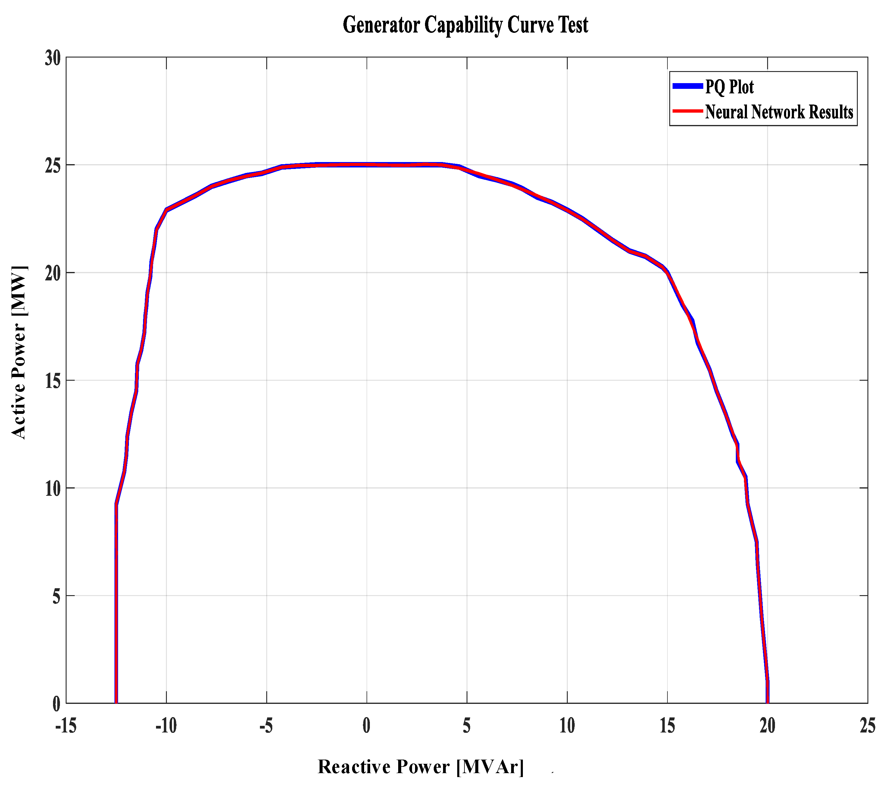
• Developing a virtual visualization of capability curve: Unlike some similar research to GCC, this study proposed a virtual visualization of GCC which can monitor the condition of generator during operation considering all the limitations of the generator.
• Shown an excellent performance: The proposed GCC is identical to the original GCC. The GCC visualization can monitor the operation condition of generator and ensure the safety of the generator through the working point of the generator.

5. Conclusions

This study successfully developed a virtual visualization of generator capability curve simulation to visualize the operation conditions of a generator. The proposed method shows an excellent performance, so it is able to obtain a capability curve that is identical to the original capability curve. The generator capability curves in this paper used a simple NN model, but the performance is excellent and the generator work point can be visualized directly to ensure the safety of the generator. Unlike other similar papers, the capability curve in this study not only can be used to evaluate the operation of the generator based on the theoretical aspects or draw it manually but is more advanced, so it is more useful for analyzing the operation condition of the generator through the working point of the generator. The virtual visualization of capability curves in this study is able to show the various possibilities that occur in the operation of a generator as they happen in reality, and it can even simulate special conditions which are based on various conditions. Based on this study, the main weakness encountered is the dependence on the original capability curve of the generator as the basis for developing the capability curve according to the proposed method. In the future, this research can be expanded by combining optimal power flow so that the analysis is more complex, where there is an optimal power flow analysis in the system in the beginning and the results of the analysis can be used for monitoring the condition of the generator through the visualization of the proposed GCC.

References

1. Shen, X.; Wu, G.; Wang, R.; Chen, H.; Li, H.; Shi, J. A self-adapted across neighborhood search algorithm with variable reduction strategy for solving non-convex static and dynamic economic dispatch problems. IEEE Access 2018, 6, 41314–41324. [Google Scholar] [CrossRef]
2. Lee, C.-Y.; Tuegeh, M. Optimal optimisation-based microgrid scheduling considering impacts of unexpected forecast errors due to the uncertainty of renewable generation and loads fluctuation. IET Renew. Power Gener. 2020, 14, 321–331. [Google Scholar] [CrossRef]
3. Fu, C.; Zhang, S.; Chao, K.H. Energy management of a power system for economic load dispatch using the artificial intelligent algorithm. Electronics 2020, 9, 108. [Google Scholar] [CrossRef] [Green Version]
4. Yang, Y.; Wei, B.; Liu, H.; Zhang, Y.; Zhao, J.; Manla, E. Chaos firefly algorithm with self-adaptation mutation mechanism for solving large-scale economic dispatch with valve-point effects and multiple fuel options. IEEE Access 2018, 5, 45907–45922. [Google Scholar] [CrossRef]
5. Nilsson, N.E.; Mercurio, J. Synchronous generator capability curve testing and evaluation. IEEE Trans. Power Deliv. 1994, 9, 414–424. [Google Scholar] [CrossRef]
6. Painemal, H.P. Enforcement of current limits in DFIG-based wind turbine dynamic models through capability curve. IEEE Trans. Sustain. Energy 2019, 10, 318–320. [Google Scholar] [CrossRef]
7. Thakar, S.; Vijay, A.S.; Doolla, S. Effect of p-q limits on microgrid reconfiguration: A capability curve perspective. IEEE Trans. Sustain. Energy 2019. [Google Scholar] [CrossRef]
8. Fernandes, I.G.; Paucar, V.L.; Saavendra, O.R. Impacts of synchronous generator capability curve in power system analyses trough a convex optimal power flow. In Proceedings of the 2019 IEEE PES Innovative Smart Grid Technologies Conference-Latin America (ISGT Latin America), Gramado, Brazil, 15–18 September 2019. [Google Scholar]
9. Sangeetha, G.; Sherine, S.; Arputharaju, K.; Prakash, S. On line monitoring of higher rated alternator using automated generator capability curve administer. In Proceedings of the 2018 International Conference on Recent Trends in Electrical, Control and Communication (RTECC), Selangor, Malaysia, 20–22 March 2018. [Google Scholar]
10. Morais, A.P. Adaptive Mho relay for synchronous generator loss-of-excitation protection: A capability curve limit-based approach. IET Gener. Transm. Distrib. 2016, 10, 3449–3457. [Google Scholar] [CrossRef]
11. Park, B.; Tang, L.; Ferris, M.C.; DeMarco, C.L. Examination of three different ACOPF formulations with generator capability curves. IEEE Trans. Power Syst. 2017, 32, 2913–2923. [Google Scholar] [CrossRef]
12. Sutherland, P.E. Safe operating limit. IEEE Ind. Appl. Mag. 2011, 17, 14–19. [Google Scholar] [CrossRef]
13. Ahmadi, H.; Foroud, A.A. Design of joint active and reactive power reserve market: A multi-objective approach using NSGA II. IET Gener. Transm. Distrib. 2015, 10, 31–40. [Google Scholar] [CrossRef]
14. Enrique, E.H. Generation capability curves for wind Farms. In Proceedings of the IEEE Conference on Technologies for Sustainability, Portland, OR, USA, 24–26 July 2014. [Google Scholar]
15. Tan, Z.; Zhong, H.; Wang, X.; Tang, H. An Efficient Method for Estimating the Capability Curve of a Virtual Power Plant. CSEE J. Power Energy Syst. 2020. [Google Scholar] [CrossRef]
16. Khazaei, J.; Nguyen, D.H.; Asrari, A. Consensus-based demand Response of PMSG wind turbines with distributed energy storage considering capability curves. IEEE Trans. Sustain. Energy 2019. [Google Scholar] [CrossRef]
17. Shicong, Y.; Ukil, A.; Gupta, A.K. Development of low voltage ride-through capability curve for grid connected diesel engine generators. In Proceedings of the IECON 2016—42nd Annual Conference of the IEEE Industrial Electronics Society, Florence, Italy, 23–26 October 2016. [Google Scholar]
18. Grainger, J.J.; Stevenson, W.D., Jr. Power System Analysis; McGraw-Hill, Inc.: New York, NY, USA, 1994. [Google Scholar]
19. Beaty, H.W.; Fink, D. Standard Handbook for Electrical Engineers, 16th ed.; McGraw-Hill, Inc.: New York, NY, USA, 2012. [Google Scholar]
20. Blackburn, J.L.; Domin, T.J. Protective Relaying Principles and Applications, 3rd ed.; CRC Press Taylor & Francis Group: New York, NY, USA, 2007. [Google Scholar]
Figure 1. Generator phasor diagram [18]: (a) over-excited generator sends reactive power to the system, (b) Excited generator absorbs reactive power from the system.
Energies 14 00185 g001
Figure 2. Phasor plot diagram in the x and y axis.
Energies 14 00185 g002
Figure 3. Plot of the phasor diagram in the power axis.
Energies 14 00185 g003
Figure 4. Phasor diagram in Figure 3 after rotating 90 ° counterclockwise.
Energies 14 00185 g004
Figure 5. Phasor diagram in Figure 4 after reflecting on the y -axis.
Energies 14 00185 g005
Figure 6. Capability curve formed from the generator phasor diagram.
Energies 14 00185 g006
Figure 7. Limitations on the generator capability curve.
Energies 14 00185 g007
Figure 8. The relationship between P m and P e .
Energies 14 00185 g008
Figure 9. Flowchart of the generator capability curve formation.
Energies 14 00185 g009
Figure 10. How to plot the capability curve.
Energies 14 00185 g010
Figure 11. Relationship between P , Q , θ , R gen , and R ref .
Energies 14 00185 g011
Figure 12. Generator capability curve testing algorithm.
Energies 14 00185 g012
Figure 13. Original capability curve from the generator in Lahendong IV geothermal power plant.
Energies 14 00185 g013
Figure 14. The developed capability curve of a generator with neural network training.
Energies 14 00185 g014
Figure 15. The developed capability curve of a generator of neural network training.
Energies 14 00185 g015
Figure 16. Original capability curve from the generator in Lahendong IV geothermal power plant.
Energies 14 00185 g016
Figure 17. Comparison of the generator capability curves for the second testing: (a) original capability curve, (b) simulation results.
Energies 14 00185 g017aEnergies 14 00185 g017b
Figure 18. Original capability curve from the generator in Lahendong IV geothermal power plant.
Energies 14 00185 g018
Figure 19. Comparison of the generator capability curves for the third testing: (a) original capability curve, (b) simulation results.
Energies 14 00185 g019aEnergies 14 00185 g019b