Article

Computational Intelligent Approaches for Non-Technical Losses Management of Electricity

Department of Electrical and Electronics Engineering, Universidad del Norte, Barranquilla 081007, Colombia
*
Author to whom correspondence should be addressed.
Energies 2020, 13(9), 2393; https://doi.org/10.3390/en13092393
Submission received: 27 March 2020 / Revised: 19 April 2020 / Accepted: 23 April 2020 / Published: 11 May 2020
(This article belongs to the Special Issue Soft Computing Techniques in Energy System)

Abstract

:
This paper presents an intelligent system for the detection of non-technical losses of electrical energy associated with the fraudulent behaviors of system users. This proposal has three stages: a non-supervised clustering of consumption profiles based on a hybrid algorithm between self-organizing maps (SOM) and genetic algorithms (GA). A second stage for demand forecasting is based on ARIMA (autoregressive integrated moving average) models corrected intelligently through neural networks (ANN). The final stage is a classifier based on random forests for fraudulent user detection. The proposed intelligent approach was trained and tested with real data from the Colombian Caribbean region, where the utility reports energy losses of around 18% of the total energy purchased by the company during the five last years. The results show an average overall performance of 82.9% in the detection process of fraudulent users, significantly increasing the effectiveness compared to the approaches (68%) previously applied by the utility in the region.

Graphical Abstract

1. Introduction

As part of real-world processes, power systems are not capable of delivering all electrical power produced to users, so a difference between the energy generated and delivered is inherent to their operation. Technically, this difference is defined as a loss of energy [1], because it is not remunerated in any way and it has environmental and economic impacts on the operation of electrical systems. Since this energy must be generated, it requires greater use of primary sources and fossil fuels in generation plants, causing over costs in the operation of the electricity network.
Losses of electrical energy can be classified into two large groups: technical losses and non-technical losses (NTL). The former corresponds to the percentage of electrical energy transformed into other types of energy during the transmission process. The second group refers to the amount of electrical energy delivered to end-users but is not billed properly and is therefore not economically represented [2,3]. In the NTL group, we find products of errors and breakdowns in measurement equipment, energy not invoiced due to errors in meter reading or billing processes, and finally, those associated with fraudulent behavior of customers, who evade payment corresponding to the consumption of electrical energy [4,5].
This paper is focused on NTL of electrical energy that are the product of fraudulent behaviors of clients. In this sense, Northeast Group LLC published a report showing that NTL frauds cause an $89.3 billion loss globally, among which $58.7 billion loss is from the top 50 emerging market countries [6]. For instance, owing to theft in electricity utilities in India, they experience a loss of nearly $4.5 billion each year. Utilities in the United State of America (USA) experience a loss of approximately $1.6-billion. In Canada, according to British Columbia Hydro (BCH), there is a loss of about $100 million each year [2,7]. In Colombia, according to the “Unidad de Planeación Minero-Energética (UPME)”, this type of loss can be assumed to account for on average 15% of the total energy purchased by the country’s electricity companies [8]. This represents a warning value due to the economic and environmental impacts that these losses bring with them, and therefore, it is important to propose solutions aimed at reducing these high rates of electrical energy losses.
Currently, commercial electrical energy companies are implementing improvement and management plans to reduce the percentage of energy lost. In this sense, statistics reflect a decrease in the percentage of non-technical losses from 20 years ago to the present [8]. Among the solutions currently implemented to detect fraud, three types stand out: consumption deviation, commercial cycle evaluation, and macro-measuring.
Consumption deviation consists of quantifying total energy losses in a specific zone and dividing this value equally among the number of users. It is then established whether the amount of energy recovered by inspecting each user of the area represents a profit for the company, taking into account the expenses associated with sending crews to check each house. The commercial cycle is a follow-up that is carried out for customers who presented drastic changes in their consumption, turning them into potential cases of irregularity. For these customers, their consumption behavior in the previous months is evaluated; as well their behavior in the same month when the change occurred but during previous years, to obtain information that makes it possible to decide with certainty whether there is a case of fraud. Finally, macro-measuring, the most used technique at the moment, consists of the placing of meters in the output of the transformers that feed groups of users. If no fraud exists, the measurement delivered by these meters must coincide with the sum of the measurements of the clients associated with that transformer. Otherwise, there are losses of energy in that group of clients.
The impact of the problem is so severe that it is currently the focus of multiple worldwide research projects, which converge towards the use of algorithms and computational intelligence techniques [3]. Such techniques facilitate the exploration, acquisition, processing, and analysis of large amounts of data, which any human being operator is not capable of, as well as a high degree of accuracy in the detection of fraud, which makes it possible to recover a large amount of the income [9,10].
Some authors tackled this problem from the perspective of intelligent algorithms and machine learning. Among the computational intelligence techniques used for the problem of fraudulent connections are neural networks [11,12,13,14], support vector machines [15,16,17], and fuzzy logic [18,19,20,21]. Such proposals demonstrate an interest in the use of these tools to obtain more rigorous and effective solutions, and confirm that these techniques become powerful tools that provide better solutions than those currently used [21,22].
In this paper, a solution is proposed through the implementation of an intelligent system to detect users with fraudulent connections, which is divided into three stages. The first stage is a clustering of consumption profiles based on a hybrid algorithm between self-organizing maps and genetic algorithms. This clustering stage is developed taking into account the consumption curve of each user. The second stage is a forecast of future consumption based on ARIMA models, which is corrected by a neural network. This prediction stage is developed taking into account customers’ consumption curves and exogenous variables such as temperature, billed days, and socio-economic stratum, among others. The final stage is a classifier of fraudulent and non-fraudulent users based on random forest, which receives as inputs the variables that characterize the consumption behavior of each user, as well as the outputs of the two stages mentioned above. The integration of clustering and forecasting techniques based on intelligent systems to identify fraudulent customers is a promising solution since the proposal allows to adapt and optimize the structure of the system for each customer. In this sense, this approach differs from those presented in other works because it seeks to reinforce detection by including additional variables that are the results of other intelligent algorithms.

2. Intelligent Approach to Managing NTL Associated with Fraudulent Connections

In this study, non-technical losses of electrical energy due to fraud by end-users are analyzed. This situation affects the operating costs of the electrical system. The result is a chain of negative effects, from economic to environmental. Therefore, this problem deserves more attention [3].

2.1. Proposed Intelligent System for Managing NTL Associated with User Fraud

To address this problem, the standard widely used model of problem-solving consists of three stages: the first one refers to the entry of the input variables, then the execution of computational intelligence techniques, and finally the detection of fraudulent users. However, the methodology developed in this research is presented in Figure 1, and it is composed of five steps.
In an attempt to relate these steps to the standard model of problem-solving, the proposed methodology is divided into three groups. The first group is marked with the blue line and contains step one (1), which corresponds to the start stage. The second group is marked with the green line and contains steps two to four (2–4), which correspond to data conditioning and execution of the intelligent system. The third group is marked with the red line and contains step five (5), which corresponds to the results stage. Next, the three groups and the methodological steps that comprise them will be described in detail.

2.1.1. Group 1: Start

This group contains the methodological step one (1). During this step, the selection of variables to characterize the problem is carried out, that is, variables with which the consumption behavior of users of electrical energy can be analyzed are defined. Based on them, it is possible to classify users as fraudulent and non-fraudulent. Table 1 shows the variables selected for the problem. These variables make it possible to analyze consumption behavior in detail. Data from these variables must be complete for all users at the system.

2.1.2. Group 2: Conditioning and Execution of the Intelligent System

This group contains the methodological steps two to four (2–4), where the conditioning and the execution of the three stages of the intelligent system are carried out. The first stage is an unsupervised grouping of similar consumption profiles. The second stage is the modeling and prediction of future consumption. The third stage is a fraudulent user detector that receives as input the outputs of the previous stages, together with the other variables described in Group 1.
Once the results of the first two stages are obtained, step three of the methodology is carried out, which corresponds to the conditioning of all the variables that enter into the final stage (stage 3). Finally, the variables already conditioned are entered into the detector in step four. This step is executed to classify users into fraudulent and non-fraudulent customers.
Figure 2 shows the proposed block diagram. The grouping and prediction stages are independent and their outputs are entered in the detection stage. Additionally, a set of inputs is used to execute stages 1 and 2, and the remaining variables are entered as inputs in stage 3 (detection). The inclusion of the grouping and prediction stages is the key difference between this proposal and others. Such variables provide information of considerable relevance that allows reinforcing the learning so that the algorithm makes a better characterization of fraudulent and non-fraudulent behaviors.

2.1.3. Group 3: Results and Validation of the System

This group contains the methodological step five (5), where the results from the analysis and validation of the detection stage are carried out. It corresponds to the evaluation of the intelligent system performance for the detection of fraudulent users.

2.2. Intelligent Detection of Fraudulent Users Using Intelligent Reinforcement Stages

This approach aims at improving performance by obtaining additional inputs from those obtained from electricity companies. These additional inputs can reinforce detection because they are the product of computational intelligence techniques that focus on characterizing aspects that are not measurable but highly significant in the analysis of electrical energy consumption behaviors. This is because of the ability of these algorithms to generalize and recognize patterns, facilitating a better and more detailed characterization of users’ behavior [10].
As a result, the addition of two reinforcement inputs to the detection is proposed, each one a product of the execution of its corresponding stage based on computational intelligence techniques. The first input is the result of the grouping stage, while the second input is the product of the prediction stage. Both stages are described below.

2.2.1. Stage 1: Unsupervised Grouping of Consumption Profiles

This process is carried out by the use of clustering algorithms. Based on the set of input variables presented in this section, users’ consumption profiles are used for the execution of this stage, resulting in a time series that represents the consumption behavior of users within the study window. The function of the cluster is to divide the set of users into groups, so that the users of the same group exhibit similar consumption behaviors, and differ from the behavior of the users of other groups (see Figure 3).
Since the function of this stage is to group according to similar consumption behaviors, it is necessary to ensure that the input variable allows the algorithm to fulfill such function. So it was decided to normalize each consumption curve (profile) concerning their maximum value to eliminate the affectation that introduces the magnitude of consumption and to capture only its behavior, as it is shown in Figure 4.

2.2.2. Stage 2: Consumption Profiles Modeling and Prediction of Next Month’s Consumption

This stage seeks to find the best model to represent the consumption profile of each user so that it is possible to perform with a high degree of certainty the prediction of the consumption of each user for the next month. For that, this stage corresponds to a regression problem, where a set of variables is used to find the function that creates the best fit for the output’s known data. In this context, some of the input variables are used to find the model that best fits the consumption profile data of each user.
The variables taken into account as inputs for this stage are (1) Consumption profile of each user, (2) Average temperature of the month, (3) Climate factor of the month, (4) User tariff, and (5) Meter readings.
Figure 5 represents the operation of the modeling and prediction stage. Given a consumption profile of a user (black line with squares) and the other variables mentioned for that user, the stage fits the model that best explains the consumption profile of this user (red line). Once this model is found, it is used to predict next month’s consumption of the user under study (red dot). The difference between the value of the red dot (prediction) and the actual value (when it occurs) is the output of stage 2 for this user, which is entered as additional reinforcement input into the detection (stage 3). This process is repeated independently for each one of the N users.

2.2.3. Stage 3: Detection of Fraudulent Users

This is the final stage of the proposed intelligent system since it is here that the intelligent detection of fraudulent users is performed. The design of this stage corresponds to the solution of a classification problem. In this context, variables that allow performing a suitable generalization of the characteristics that differentiate fraudulent users from non-fraudulent ones are used. In addition to these variables, the outputs of stages 1 and 2 are also used as inputs for this stage, since these represent the reinforcement inputs whose purpose is to improve the characterization of the consumption behavior provided by the initially mentioned variables.
The variables taken into account as inputs for this stage are: (1) User measurement equipment, (2) Geographic location of the user, (3) Number of complaints made, (4) Number of overdue bills, (5) Customer fraud history, (6) Reading and billing anomalies, (7) Group to which each user belongs–output of stage 1– and 8) Consumption deviation–output of stage 2.
The classification problems belong to the supervised learning approach. Therefore, the training of the intelligent technique is performed by examples with known results. To achieve the training of the intelligent classifier for the detection of fraudulent users, not only are the mentioned inputs used but a set of known outputs for the combinations of inputs are used as well. This is the purpose of the variable balance and moorage of macrometers, as well as the variable results of campaigns and inspections. These make it possible to determine whether a user shows normal or fraudulent behavior so that the classifier can be trained with the examples determined by the sets of inputs and their outputs.
Figure 6 shows an example of the operation of the detection stage. A set of examples is initially presented, which corresponds to a group of users whose input variables are known, as well as their corresponding output (normal or fraudulent). The data of these users are entered to train the classification algorithm, which at the end of the process is able to determine if one user is committing fraud or not, depending on the values of their inputs.

2.3. Implementation of the Intelligent System for the Detection of Fraudulent Users

The proposed approach is a general methodology that is composed of a series of steps whose correct execution allows the detection of fraudulent users. Although the approach can be applied generally to any system of electric power distribution; for convenience, the place where this research is developed is the city of Barranquilla, Colombia. The inputs of the system are (1) User consumption profile including a series of 55 periods, (2) Average temperature of the month for 55 periods, (3) Climate factor of the month for 55 periods, (4) User tariff (fixed), and (5) Billed days of the month for 55 periods.

2.3.1. Implementation of the Stage of Unsupervised Grouping of Consumption Profiles (Stage 1)

The two most widely used techniques for solving clustering problems are self-organizing maps (SOM) and K-Means. For the implementation of this stage, it is decided to use SOM. The SOM parameters are (1) dimension, which is related to the total number of groups obtained from the grouping; (2) topology, which is the interconnection of the neurons on the map; (3) distance function, being the membership of each element in any of the groups in the network; (4) the number of training steps, which makes use of the space covered by the elements to be grouped [23].
To improve the results of this method, it is necessary to perform the best possible grouping, which implies what combination of parameters makes such clustering possible. A search algorithm is used since this type of technique makes it possible to find the best possible solution. A genetic algorithm (GA) is the metaheuristic technique selected [10].
The SOM is responsible for grouping consumption profiles for a given configuration of its parameters, while the genetic algorithm explores the combinations of possible parameter configurations until it finds the one that yields the best clustering. During the operation of this stage, the GA follows its operating principle to select the combinations of parameters with which the SOM is executed. The functional structure of the stage is presented in Figure 7.

2.3.2. Implementation of the Stage of Consumption Profiles Modeling and Prediction of the Next Month Consumption (Stage 2)

The second stage consists of two parts: the first is obtaining the best ARIMA model for each user of the system. These models are obtained by using the Akaike Information Criterion (AIC), which allows the selection of P and Q values that yield the best model in terms of performance and complexity. Once the models that represent each user are obtained, the consumption of the next month is predicted for each of them [24]. Figure 8 shows that even the best model obtained is not able to perfectly explain the behavior of the consumption profile. This is because ARIMA models are univariate models of time series, that is, they try to explain the series with a single input variable, which is the same series. In the particular case of the consumption of electrical energy, some factors modify the consumption behaviors of users. These factors are known as exogenous variables. The consumption profile is not able to explain itself. Therefore, these exogenous variables can explain the differences between both curves.
The second part of the second stage uses neural networks to intelligently correct each user model obtained during the first part. This is done by selecting the best neural network to explain, from the exogenous variables, the differences in each statistical model of the users. The prediction of the next consumption is also affected by the correction.
Obtaining the differences corresponds to a problem of regression that, without having an analytical solution model, favors the use of computational intelligence techniques. The intelligence technique selected must belong to supervised learning, because all the differences are known for 55 periods, which in this case represent the output. The inputs are the average temperature of the month, climate factor of the month, user tariff, and days billed in the month for each of the 55 periods of the study window, which correspond to the exogenous variables of the model. Based on the above, the set of examples that can train an intelligent algorithm in a supervised way is complete.
Currently, the two most widely used techniques for regression problems are neural networks and support vector machines (SVM). The technique selected for the second part of this stage is artificial neural networks (ANN), which is a feed-forward multi-layer perceptron with training based on backpropagation. The neural network is randomly initialized before training, which makes it possible to obtain solutions that can be completely different, even with the same initial data conditions. This variability factor facilitates the exploration of an extensive set of solutions, opening the possibility of finding networks that generalize quite well and give way to obtaining better solutions. Several neural networks are trained independently of each other, and the one with the best performance is selected for obtaining the differences.
At the output of this stage, differences added to the statistical model in each period to perform the correction are obtained. Figure 9 shows an example of the intelligent correction process. Here, the intelligently corrected model succeeds in satisfactorily explaining the behavior of the user profile.
Finally, statistically and intelligently corrected predictions are compared to determine which of them is accepted as valid for each user of the system. The one that is closest to the actual value of the customer profile is selected to calculate the deviation of the consumption. The functional structure of the stage is shown in Figure 10.
The aspects taken into account to obtain the statistical model of each user of the system are shown below:
  • Verification of stationarity: ARIMA models are suitable for non-stationary series. The verification of stationarity is carried out by using the statistical test of Dickey-Fuller.
  • Limits of the P and Q degrees of the polynomial model: This value indicates the non-existence of the part of the model whose degree is zero. The maximum value for these coefficients is given by the number of observations that exist from the time series to be modeled. The tests show that the maximum value for P and Q from the 55 observations that compose the study window is two in both cases.
  • Selection of P and Q values for each user’s model: As mentioned, the Akaike criterion makes it possible to select the best model based on its performance and complexity [24,25]. For the ARIMA models, the criterion measures the performance of the fitting by the likelihood of the model. To measure the complexity, the criterion quantifies the number of parameters of the model; this is represented by the sum of its degrees of P and Q. Equation (1) shows the AIC expression used to evaluate the models, where LH is the likelihood and NumParam is the sum of P and Q.
AIC = 2 ( LH ) + 2 ( NumParam )
For each user, the models with degrees 1 and 2 are tested for both P and Q. For each model, its respective AIC is calculated. The model with the lowest AIC value is the best. Table 2 exemplifies the AIC calculation for each possible model.
The aspects taken into account to perform the intelligent correction of the statistical models of each user of the system are shown below:
  • The number of neurons in the hidden layer: This parameter is closely linked to the performance of the neural network. A low number of neurons will lead to poor performance, while a very high number can lead to overfitting [24]. To obtain this parameter, there are several heuristics according to empirical rules. Equation (2) shows the most common one.
N H i d d e n = [ ( 2 3 ) N i u t p u t ] + N O u t p u t
where N i n p u t is the number of neurons in the input layer, which corresponds to the number of input variables, six in the case of the second part of the stage. N O u t p u t is the number of neurons in the output layer, which is given by the number of outputs of the network. As for each case of the network execution, the values of the six inputs for a period make it possible to obtain as output the difference in the said period between the real series and the statistical model; there is only one exit. Therefore, N O u t p u t is one for the case of the second part of this stage.
The evaluation of the expression shows that N H i d d e n is five for all networks to use within the second part of stage 2.
  • The number of neural networks: the use of an ANN introduces variability in the results, even though it is executed with a fixed configuration. This happens when the problem is not easy to solve, allowing the network to learn differently in each execution. To take advantage of this feature, 50 independent networks are trained for each user. The network with the best performance is selected for the intelligent correction of the statistical model of that user.
  • Neural network performance metrics: A metric based on the linear correlation coefficient is used for the evaluation of each trained network. A way to evaluate the fit of a model is by calculating the correlation coefficient between the actual data and the fitted model data. The higher the value of the correlation coefficient, the better the fitting performed by the model [25].
Since the data of the input variables are divided into three groups (training, validation, and testing), the linear correlation coefficient for each group is calculated. The performance of a network is better the higher the calculated value (see Equation (3)).
P e r f = C T r a 2 + C V a l 2 + C T e s t 2
where C t r a is the linear correlation coefficient of the fitting performed by the network for the training data, C V a l is the linear correlation coefficient of the fitting performed by the network for the validation data, and C T e s t is the linear correlation coefficient of the fitting performed by the network for test data. To obtain the definitive differences of a user, the network whose P e r f value is higher than the other 49 is used.

2.4. Implementation of the Stage of Fraudulent User’s Detection (Stage 3)

All the efforts made to implement the two previous stages converge at this point. This stage uses the data of the variables it receives as inputs to generalize about the patterns and behaviors that differentiate a fraudulent user from a non-fraudulent one. For each user, the output of this stage is a label that allows classification (fraudulent and non-fraudulent).
The input variables used for the execution of this stage are: (1) User measurement equipment, (2) Geographic location of the user, (3) Number of complaints in the last year, (4) Number of overdue bills, (5) Customer fraud history, (6) Reading and billing anomalies in the last year, (7) Group to which each user belongs—output of stage 1—and (8) Consumption deviation of the month—output of stage 2.
Since the execution of the system to detect fraudulent users is done monthly, the variable consumption deviation is composed of the deviations of users for the month in which the detection of fraud is desired. The variables number of complaints and reading and billing anomalies are evaluated for the last 12 periods before the month of execution of the system, this is because they represent user behaviors that can change with the time. The variables user measurement equipment, geographic location, and group to which the user belongs are fixed. Likewise, the variable customer fraud history and number of overdue bills result from evaluating the user throughout the study window.
The computational intelligence technique used for supervised user classification is random forests. The output is a label for each user where the class is indicated (fraudulent and non-fraudulent). The functional structure of the stage is presented in Figure 11. Arrows with dotted lines indicate that this part of the process occurs only during training, and it is not taken into account during the commissioning of the system.

3. Experimental Results

3.1. Tests and Results of Stage 1: Grouping of Consumption Profiles

The hybrid design between the clustering technique and the genetic algorithm is proposed to find the best possible grouping. Next, the tests for the establishment of the upper limit of the dimension parameter are presented, as well as the results of the execution of the stage.

3.1.1. Selecting the Upper Limit of the SOM Dimension Parameter

The selection of the upper limit for the SOM dimension parameter is experimentally established. Likewise, a criterion is established to increase the performance of the stage without falling into individualization. This criterion consists in finding the groups with a greater and smaller number of elements after the grouping. If the number of elements in the minor group does not exceed 5% of the number of elements of the major, the grouping is considered invalid.
The tests consisted of the successful execution of the SOM by varying the upper limit of the dimension parameter. It is initiated from the value of the lower limit that is two (four groups). The grouping is carried out and the established criterion is applied to evaluate the results. The same configuration is tested 10 times to take into account the variance of the process. If the results obtained from the configuration under study met the criterion, the value of the upper limit is increased by one and the process is carried out again.
The tested upper limit values met the criteria with no problem in all of their replicates until 15 (225 groups). In 16 (256 groups), of the 10 tests performed, five met the criteria and the other five did not, and in 17 (289 groups), none of the 10 SOM execution results are accepted. Therefore, it is decided to set the value of the upper limit in 16, to include those results that fulfill the condition for this value.

3.1.2. Optimization Results

The execution of stage 1 of the system concludes when the optimization process is finished. The optimization performed is multi-objective, in which it seeks to obtain the least number of groups and the best performance. The multi-objective optimization processes do not yield a single solution; they yield a set that contains the best solutions for each objective function. The set containing the best solutions for each objective function is known as the Pareto frontier. The completion of the GA yields the Pareto frontier with the best solutions to the problem. For system automation, the algorithm chooses by default the solution with the best value of the proposed performance metric. The results obtained from the final execution of this stage are presented, which is performed with the total users of the system (92,794). The solution space consists of 360 combinations of the SOM configuration parameters, the GA has to evaluate 217 of these combinations to reach the solution of the optimization. This validates the decision to use this metaheuristic technique over an experimental design. The Pareto frontier after the execution of the stage for the total set of users is shown in Figure 12.
Table 3 contains the values of the two objective functions that compose the Pareto frontier.
The Pareto frontier does not include the value of the upper limit of the parameter dimension (16). The “chromosomes” of the GA that included this value do not meet the proposed criterion of the minimum number of elements in a group.
The default selection of the solution is made with the best value of the proposed performance metric, which corresponds to the point of the frontier that leads to the obtaining of 225 groups and the lowest value of the metric (0.1392). The values of the SOM parameters that describe the configuration representing that frontier point are:
  • Dimension: 15 × 15 neurons (225 groups).
  • Topology: Grid.
  • Distance function: “boxdist.”
  • Number of training steps: 100.
The grouping is obtained from the execution of the SOM with the configuration described above. The group with the highest number of elements has 1237, while the group with the lowest number of elements has 140; this value is 11.1% of 1237. Therefore, it fulfills the criterion of the minimum number of elements. The consumption profiles are composed of 55 periods and correspond to the curves with blue lines. The red line corresponds to the average profile of each group. Examples of selected groups are shown in Figure 13, Figure 14, Figure 15 and Figure 16.

3.2. Tests and Results of Stage 2: Modeling and Prediction of Consumption Profiles

The first one is statistical modeling of consumption profiles, where an ARIMA model is fitted for each user of the system. These models must correspond to the model that best explains the profile of each user. To achieve this, the Akaike Information Criterion is used, which makes it possible to compare ARIMA models of different orders and select one with suitable performance and acceptable complexity.
In an attempt to improve the fitting made by the statistical models, the second part of the stage is implemented, which trains a set of 50 independent neural networks to select the one that can better explain the differences between the actual consumption and the fitted model. Like the first part, this second part is also executed individually for each user.
Next, the tests performed on each of the parts of stage 2 are described. This is done to evaluate the performance and validate the functioning of these parts. Since both parts are independent of each other, the tests and experiments, as well as the analysis of the results obtained, are separately presented.

3.2.1. Obtaining the Statistical Model of Each User

After validating the stationarity of the profile of each user through the Dickey-Fuller test, the corresponding four statistical models are fitted for each user. This is done since the combinations (1,1), (1,2), (2,1) and (2,2) of the degrees P and Q of the polynomials of the model are tested. Subsequently, the best of the four ARIMA models fitted is selected, using the Akaike Information Criterion. Although the AIC makes it possible to select the best model based on the likelihood and complexity of the model, the most commonly used metric to evaluate the performance of curve-fitting models is the Mean Absolute Percentage Error (MAPE) (see Equation (4)) [26].
M A P E = 100 n t = 1 n | A t F t A t |
where n is the number of observations in the series, A t is the actual value at time t, and F t is the value fitted by the model at time t. This metric is used to quantify the performances of the statistical models obtained for each user and is the product of the first part of this stage. The above is carried out in order to have a metric to evaluate the performance of the statistical modeling from a general perspective, which is used to validate the operation of this first part of the stage as a whole.
As the execution of this first part is individual for each user, a total of 92,794 ARIMA models are obtained. Due to the impossibility of showing all of them in this paper, a selected sample of four users is presented in Figure 17, which makes it possible to verify the functionality of this part of stage 2.
The average of the MAPE of the 92,794 users is 15.42%. To support the above statement, the frequency histogram of Figure 18 is presented, which shows the ranges within which the MAPE for all users is located.
The range with the highest number of MAPE is between 10% and 11%, containing 7292 users. This, together with the analysis of the MAPE average, makes it possible to validate the operation of this part of stage 2, because of its satisfactory performance in the modeling of the consumption profiles of the users.

3.2.2. Intelligent Correction of the System Users’ Models

For each user, the correction is done by implementing a set of neural networks that are independent of each other. These networks are trained to be able to explain the differences between the user’s actual consumption profile and its corresponding fitted statistical model. To evaluate the performance of each network, a metric based on the linear correlation coefficient is used, and the network with the best performance is selected to obtain the differences that must be added to the statistical model in each period, to correct its fitting for the user under study.
The selection of the neural networks as a technique to implement the second part of this stage is explained. The main idea is to take advantage of the high variability that this technique presents in its output to explore a wide number of solutions to find a neural network that can correctly generalize the behavior of the differences in each period of the study window, starting from the relations and interactions between the inputs of this second part of the stage (exogenous variables). It is then necessary to carry out an experiment that tests a varied number of networks, until finding one with the desired behavior.
The three factors that can be varied for the execution of this type of network are the training algorithm, the number of neurons of the hidden layer, and the number of networks tested [27]. The training algorithm is defined as fixed, selecting one that takes longer in execution but yields better results (Bayesian regularization). The number of neurons in the hidden layer remained fixed and is obtained by means of a heuristic, which avoided overfitting and underfitting. Therefore, the only factor varied is the number of trained networks.
To carry out the experiment, a set of neural networks are trained, all with the same configuration. Although all have the same configuration, the high variability of the technique makes it possible to obtain a diverse set of outputs. It is defined that 50 equal networks are trained for each user.
The performance metric for the evaluation of the implemented neural networks is defined, namely to obtain the linear correlation coefficient for each data set (training, validation, and testing). These coefficients make it possible to analyze the performance of a network for each set. The evaluation of the overall performance of the said network is analyzed by computing the square sum of the three previous coefficients, which corresponds to the performance metric selected.
Next, the process of selecting the best network for a system user is exemplified. Because this part of the stage analyzes each user individually, this process is repeated in the same way for all users of the system. Therefore, the example presented is sufficient, and it is not necessary to show the process for all (92,794 users).
Figure 19 shows the linear correlation coefficients of the datasets for each of the 50 networks implemented during the analysis of the sample user. Figure 20 shows the performance metric for each network. The best network is the one where the highest point of the curve occurs, which is indicated with a red dotted line. The maximum value mentioned occurs in network number 37, which is selected to perform the intelligent correction of the statistical model of the sample user.
After selecting the best network, it is executed to perform the intelligent correction of the statistical model obtained for that user. The execution of the network makes it possible to obtain the differences that must be added to the statistical model in each period to improve the fitting (see Figure 21). As this process occurs in the same way for the 92,794 users, a sample of four users is selected to demonstrate the operation of this second part of stage 2. The results of the correction for these users are shown in Table 4. The selected examples correspond to users where the statistical model does not present a good performance, which makes it possible to notice the action of intelligent correction.
The output of the stage of the prediction selection for each user is the consumption deviation, i.e., the difference between the closest prediction and the actual consumption of the predicted month for each of them. After the execution of stage 2, predictions are made for each user: one by the statistical models and one corrected by the neural network. Although it is verified that the intelligent correction part works correctly, it is evident that in all users the performance is not improved. Therefore, in all cases, the corrected prediction is not more accurate. The above represents the reason why it is decided that the comparison of both predictions with the actual value is made, to select the closest one.
After the execution of the entire stage, the number of users for whom the intelligent correction improves the statistical fitting (decreases the MAPE) is 76,451. This corresponds to 82.38% of the total users of the system. However, when comparing the predictions, the situation changes. Despite the good performance of the intelligent correction, only in 36.26% does it manage to make a more accurate prediction. Nevertheless, the result obtained is satisfactory. This is because it is possible to improve 36.26% of the predictions using intelligent correction, which is not possible using only the statistical prediction.

3.3. Tests and Results of Stage 3: Fraudulent User Detection

Once the sample dataset for the training is available, the functionality of the stage consists of the execution of the intelligent classification algorithm. Therefore, the tests are oriented towards the selection of the classification technique and the configuration of its parameters to obtain the best possible classification.

3.3.1. Selection of the Intelligent Classification Technique

In Section 2.3, three techniques are considered for the implementation of this stage. These techniques are artificial neural networks, support vector machines, and random forests. The one with the best performance for solving the problem of the classification of users into fraudulent and non-fraudulent is selected. An experiment is executed to compare the three techniques, where the evaluation of their performance is carried out by the most commonly used method to evaluate classification algorithms, which is known as the K-fold cross-validation [28].
To describe it briefly, K-fold cross-validation divides the total set of training data into K equal (or roughly equal) groups. K-1 groups are used to train the algorithm, the remaining group is used for testing, the algorithm is executed, and the results are recorded (performance). Next, K-1 groups are used once more to train the algorithm a second time, and the remaining group is reserved for testing. In this second run, the group that is first used for testing must be part of the K-1 used for the training, with a different group used for testing. The process is repeated until the K groups are used for testing, i.e., the technique is executed a total of K times. The overall performance of the classification algorithm is the average of the performances that are obtained for each of the K testing groups.

3.3.2. Experiment to Select the Classification Technique

The number of periods (months) for training the detector is six (November 2017 to April 2018). The set of examples that results from examining these periods consist of 4640 users. This amount is considerably smaller than the 92,794 total users of the system. However, this is explained because the sample base is constructed from the variables of macrometers (non-fraudulent users) and inspection results (fraudulent users).
The electricity company of the region carries out between 20,000 and 30,000 monthly customer inspections. This number is the total for the entire Caribbean region. It is reasonable to assume that the number of monthly inspections carried out for users belonging to the Barranquilla delegation is well below the total number presented. Besides, the total number of users of the system is the product of a series of filters. Therefore, of all inspections carried out in Barranquilla, those that encounter valid users of the system are even smaller. All of the above explains the reason why only 4640 users are obtained after reviewing the six periods for the training of the detector.
One of the conditions for the correct training of a classification algorithm is to guarantee the homogeneity of the training base, that is, to have an equal number of examples of each class. This is done so the algorithm can perform a good generalization since highly unbalanced training sets (with an appreciable difference between the number of examples for each class) tend to present bias in learning towards classes with more examples.
From the above, it is possible to infer that of the 4640 training examples, 2320 are fraudulent users and the remaining 2320 are non-fraudulent. On average, 750 users are provided monthly to feed the bank of examples of training: approximately 375 of each class (fraudulent and non-fraudulent).
The experiment performed for the comparison of the three techniques is K-fold cross-validation with a K of 10, which is executed three times (one time for each technique). The complete base of 4640 users is used for the experiment, which means that 10 groups of 464 users are obtained for cross-validation, with each round using 9 for training (4176 users) and 1 for validation (464 users).
The network topology, number of neurons of the hidden layer, and the training algorithm are fixed for the configuration of the neural network. The topology is a two-layer feed-forward; the number of neurons is obtained by the expression presented in Equation (4), and the training algorithm corresponds to the best performance (in classification problems) with longer training time. The parameter varied is the number of times training the network, that is to say, the same network is trained several times to find the one with the best results. To configure the SVM, the Kernel function is fixed, using the most common Kernel for classification problems. Gamma coefficient and cost are varied. To configure the random forest, the parameter varied is the number of trees.
A set of tests is performed to determine the values of the parameters of each technique that make it possible to obtain suitable results for the training dataset. Table 5 compiles the values of the fixed and variable parameters of each technique.
Table 6 compiles the K-fold cross-validation with 
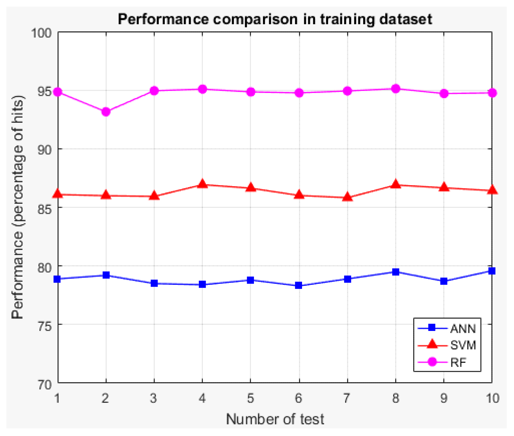
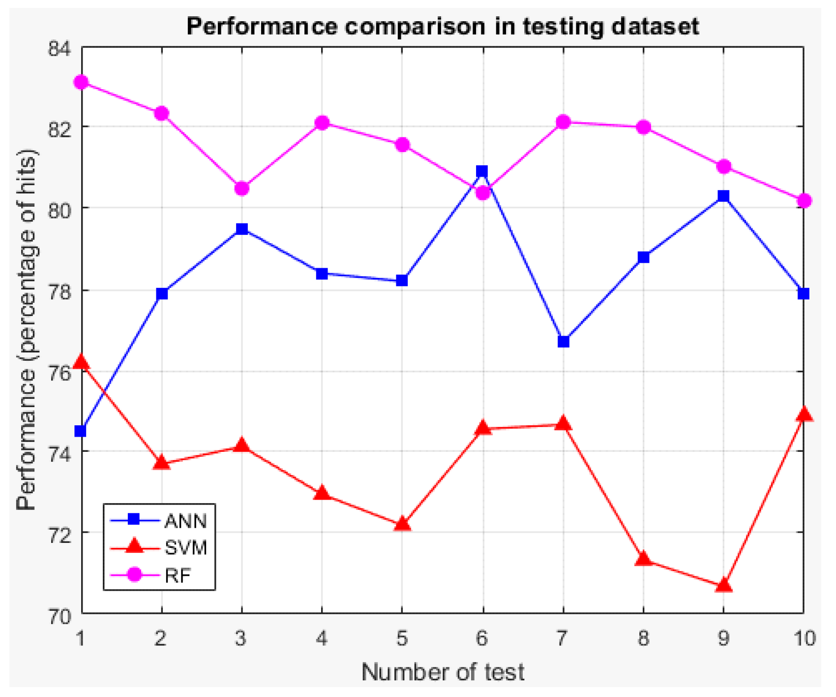
K of 10 results for the three techniques, which show the training and testing performances for each one of the 10 rounds. The performance represents the success rate (percentage of hits) of each technique, i.e., in what percentage of the times it indicates as fraudulent a fraudulent user and as non-fraudulent a non-fraudulent user.
The values below in bold indicate the technique with the highest average performance for each case (training and testing), which shows that for both cases, the random forest is the technique with the best average performance. Therefore, it is the technique selected for the implementation of the classifier of stage 3. Additionally, for both cases, graphs showing the performances of the techniques for each round of K-fold cross-validation are presented (See Figure 22 and Figure 23).
Once random forests are selected as the technique to be used, it is necessary to find the values of the parameters of the random forest that made it possible to obtain the best performance of the classification. As mentioned previously, for this technique, the only parameter that can be varied is the number of trees of the model. Therefore, an experiment based on K-fold cross-validation is performed once more to determine the number of trees that could obtain the best performance.
K-fold cross-validation is used with K of 5; the decrease in the value of K is justified in the low variability of the output of the technique (see Figure 22 and Figure 23). The total training base (4640 users) is used to carry out the experiment. This means that five groups of 928 users each are obtained for cross-validation, using four in each round for training (3712 users) and one for validation (928 users). The number of trees to test ranged from 10 to 100 in steps of 10.
A total of 10 K-fold cross-validations are performed with K of 5 since for each value of the number of trees, it is necessary to obtain the general performance of the technique. Figure 24 compiles the average performance results for each number of trees in training and testing cases.
From the presented results, the value of 60 is selected for the parameter of the number of trees of the model. The best average performance of the training is the model of 90 trees, with 95.7%; the model of 60 trees has the second-best average performance in the training, with 95.6%. However, in the testing scenario, the 90-tree model has the lowest average performance, with 81.36%, while the 60-tree model has the highest average performance, with 82.87%. Because of the small difference in the training case and the big difference in the testing, the 60-tree model performs best.

3.3.3. Selection of the Number of Trees

Based on the experiment carried out to select the number of trees, the model of 60 trees is obtained and trained with the training dataset of 4640 users (six periods). Stage 3 and the system validation are performed through the execution of the detector in the three periods reserved for testing (May 2018 to July 2018). The execution of the system is done monthly; therefore, each period is independently tested. The extraction of the users from each test period makes it possible to obtain three sets of data, which are summarized in Table 7. However, although some of them are not perfectly homogeneous; the difference is minimal and does not have any impact on the execution of the system.
A confusion matrix is used to evaluate the system performance in each testing set (see Table 8). The three sets (i.e., periods reserved for testing) are not used during training, so they are completely new and unknown to the system. The results of these sets are known and used to compare them with those obtained from the execution of the system.
The performance (percentage of hits) of the classification for the first period is 82.9%. Of the 494 fraudulent users, the detector identified correctly 423, missing 71 users. Of the 513 non-fraudulent users, the detector identified correctly 412, missing 101 users.
The performance (percentage of hits) of the classification for the second period is 82.7%. Of the 453 fraudulent users, the detector identified correctly 386, missing 67 users. Of the 461 non-fraudulent users, the detector identified correctly 370, missing 91 users.
The performance (percentage of hits) of the classification for the third period is 83.1%. Of the 549 fraudulent users, the detector identified correctly 470, missing 79 users. Of the 549 non-fraudulent users, the detector identified correctly 442, missing 107 users.

4. Conclusions

The results obtained from the execution of the proposed intelligent system made it possible to identify its striking characteristics and those of each stage that compose it. It was possible to evaluate the performance of the system in achieving the main objective for which it was designed, which is the detection of users with fraudulent behavior. Concerning the above, the system has an average overall performance of 82.9% in identifying correctly the class to which each evaluated user belongs. However, because this process is composed of multiple stages, it is necessary to reflect on each part that has made it possible to achieve the performance mentioned. Many variables were selected to characterize the electrical energy consumption behavior of the users under study. However, the objective was not to select a large number of variables but to identify those that provide the greatest amount of information to complete the characterization. A key role was played by the decision to take into account the experience of people who work in the electricity companies because it led to the selection of the variables.
Although the clustering of consumption profiles was used by several authors reviewed in Section 1, the method in this proposal was optimized by the use of a genetic algorithm. In this sense, the results from this grouping process improve with the best configuration performance.
Essentially, the approach of stage 2 was oriented towards obtaining a correct prediction of customers’ consumption. This was carried out through a statistical block that adjusted the best model of each user, from which an average general MAPE of 15.42% was obtained. Next, an intelligent correction of the statistical models was performed, which reduced the average general MAPE to 12.83%, which led to a performance increase in the prediction of 36.26%.
Classification problems require the use of a technique capable of recognizing the patterns present in the data. To ensure the correct solution to the problem of detecting fraudulent users, several techniques were compared, and the one that presented the best performance was selected (random forests). This led to the achievement of the mentioned performance of 82.9%, which was considered satisfactory and made it possible to validate the operation of the system.

Author Contributions

Conceptualization, R.G.R.; data curation, R.G.R.; formal analysis, R.G.R.; investigation, R.G.R. and C.G.Q.M.; methodology, R.G.R. and C.G.Q.M.; project administration, C.G.Q.M.; software, R.G.R. supervision, J.J.M. and C.G.Q.M.; validation, R.G.R., J.J.M. and C.G.Q.M.; visualization, R.G.R., J.J.M. and C.G.Q.M.; writing—original draft, R.G.R., J.J.M. and C.G.Q.M.; writing—review and editing, J.J.N. and C.G.Q.M. All authors have read and agreed to the published version of the manuscript.

Funding

This research received no external funding.

Acknowledgments

This work was supported by Universidad del Norte, Barranquilla-Colombia.

Conflicts of Interest

The authors declare that there are no conflicts of interest regarding the publication of this paper.

References

  1. Navani, J.P.; Sharma, N.K.; Sapra, S. Technical and non-technical losses in power system and its economic consequence in Indian economy. Int. J. Electron. Comput. Sci. Eng. 2012, 1, 757–761. [Google Scholar]
  2. Ahmad, T.; Chen, H.; Wang, J.; Guo, Y. Review of various modeling techniques for the detection of electricity theft in smart grid environment. Renew. Sustain. Energy Rev. 2018, 82, 2916–2933. [Google Scholar] [CrossRef]
  3. Bula, I.; Hoxha, V.; Shala, M.; Hajrizi, E. Minimizing losses with point-to-point losses with measurement of voltage drop losses between SMART meters. IFAC 2016, 49, 206–211. [Google Scholar]
  4. Suriyamongkol, D. Non-Technical Losses In Electrical Power Systems. Ph.D. Thesis, Ohio University, Athens, OH, USA, November 2002. [Google Scholar]
  5. Viegas, J.L.; Esteves, P.R.; Melício, R.; Mendes, V.M.F.; Vieira, S.M. Solutions for detection of non-technical losses in the electricity grid: A review. Renew. Sustain. Energy Rev. 2017, 80, 1256–1268. [Google Scholar] [CrossRef] [Green Version]
  6. Han, W.; Xiao, Y. NFD: Non-technical loss fraud detection in Smart Grid. Comput. Secur. 2017, 65, 187–201. [Google Scholar] [CrossRef] [Green Version]
  7. Razavi, R.; Gharipour, A.; Fleury, M.; Justice, I. A practical feature-engineering framework for electricity theft detection in smart grids. Appl. Energy 2019, 238, 481–494. [Google Scholar] [CrossRef]
  8. Unidad de Planeación Minero Energética (UPME). Plan Preliminar de Expansión de Referencia Generación—Transmisión 2011–2025; UPME: Bogotá, Colombia, 2011. [Google Scholar]
  9. Ma, H.; Shen, S.; Yu, M.; Yang, Z.; Fei, M.; Zhou, H. Multi-population techniques in nature inspired optimization algorithms: A comprehensive survey. Swarm Evol. Comput. 2019, 44, 365–387. [Google Scholar] [CrossRef]
  10. Zhang, J.; Oluwarotimi, S.; Wang, H. Sustainable computing: Informatics and systems intelligent computing system based on pattern recognition and data mining algorithms. Sustain. Comput. Inform. Syst. 2018, 20, 192–202. [Google Scholar]
  11. Ahmad, T. Non-technical loss analysis and prevention using smart meters. Renew. Sustain. Energy Rev. 2017, 72, 573–589. [Google Scholar] [CrossRef]
  12. Cabral, J.E.; Pinto, J.O.P.; Martins, E.M.; Pinto, A.M.A.C. Fraud detection in high voltage electricity consumers using data mining. In Proceedings of the 2008 IEEE/PES Transmission and Distribution Conference and Exposition, Chicago, IL, USA, 21–24 April 2008; pp. 3–7. [Google Scholar]
  13. Galván, J.R.; Elices, A.; Muñoz, A.; Czernichow, T. System for Detection ff Abnormalities and Fraud in Customer Consumption. In Proceedings of the 12th Conference on the Electric Power Supply Industry, Pattaya, Thailand, 2–6 November 1998. [Google Scholar]
  14. Guerrero, J.I.; León, C.; Member, I.; Biscarri, F.; Monedero, I.; Biscarri, J.; Millán, R. Increasing the efficiency in non-technical losses detection in utility companies. In Proceedings of the Melecon 2010—2010 15th IEEE Mediterranean Electrotechnical Conference, Valletta, Malta, 26–28 April 2010; pp. 136–141. [Google Scholar]
  15. Yap, K.S.; Tiong, S.K.; Nagi, J.; Koh, J.S.P.; Nagi, F. Comparison of supervised learning techniques for non-technical loss detection in power. In International Review on Computers and Software (I.RE.CO.S.); Praise Worthy Prize: Rome, Italy, 2012. [Google Scholar]
  16. Nizar, A.H.; Dong, Z.Y. Identification and detection of electricity customer behaviour irregularities. In Proceedings of the 2009 IEEE/PES Power Systems Conference and Exposition, Seattle, WA, USA, 15–18 March 2009; pp. 1–10. [Google Scholar]
  17. Pok, H.L.; Yap, K.S.; Hussien, Z.F.; Mohamad, A.M. Abnormalities and fraud electric meter detection using hybrid support vector machine and modified genetic algorithm. In Proceedings of the 19th International Conference on Electricity Distribution, Vienna, Austria, 21–24 May 2007; pp. 21–24. [Google Scholar]
  18. Babu, T.V.; Murthy, T.S.; Sivaiah, B. Detecting unusual customer consumption profiles in power distribution systems—APSPDCL. In Proceedings of the 2013 IEEE International Conference on Computational Intelligence and Computing Research, Enathi, India, 26–28 December 2013; pp. 1–5. [Google Scholar]
  19. Angelos, E.W.S.D.; Saavedra, O.R.; Cortés, O.A.C.; De Souza, A.N. Detection and identification of abnormalities in customer consumptions in power distribution systems. IEEE Trans. Power Deliv. 2011, 26, 2436–2442. [Google Scholar] [CrossRef]
  20. Muniz, C.; Vellasco, M.; Tanscheit, R.; Figueiredo, K. A neuro-fuzzy system for fraud detection in electricity distribution. In Proceedings of the 2009 International Fuzzy Systems Association World Congress and 2009 European Society of Fuzzy Logic and Technology Conference IFSA-EUSFLAT 2009, Lisbon, Portugal, 20–24 July 2009; pp. 1096–1101. [Google Scholar]
  21. Viegas, J.L.; Esteves, P.R.; Vieira, S.M. Clustering-based novelty detection for identi fi cation of non-technical losses. Electr. Power Energy Syst. 2018, 101, 301–310. [Google Scholar] [CrossRef]
  22. Messinis, G.M.; Hatziargyriou, N.D. Review of non-technical loss detection methods Decision tree False positive. Electr. Power Syst. Res. 2018, 158, 250–266. [Google Scholar] [CrossRef]
  23. Benghabrit, A.; Bouhaddou, I. A survey of clustering algorithms for an industrial context A survey of clustering algorithms for an industrial context. Procedia Comput. Sci. 2019, 148, 291–302. [Google Scholar]
  24. Bengtsson, T.; Cavanaugh, J.E. An improved Akaike information criterion for state-space model selection. Comput. Stat. Data Anal. 2006, 50, 2635–2654. [Google Scholar] [CrossRef]
  25. Mehta, P.; Bukov, M.; Wang, C.; Day, A.G.R.; Richardson, C.; Fisher, C.K.; Schwab, D.J. A high-bias low-variance introduction to Machine Learning for physicists. Phys. Rep. 2019, 810, 1–124. [Google Scholar] [CrossRef] [PubMed]
  26. Adhikari, R.; Agrawal, R.K. A combination of artificial neural network and random walk models for financial time series forecasting. Neural Comput. Appl. 2014, 24, 1441–1449. [Google Scholar] [CrossRef]
  27. César, C.; Ramos, O.; De Sousa, A.N.; Papa, J.P.; Falcão, A.X. A New Approach for Nontechnical Losses Detection Based on Optimum-Path Forest. IEEE Trans. Power Sys. 2011, 26, 181–189. [Google Scholar]
  28. Refaeilzadeh, P.; Tang, L.; Liu, H. Cross-Validation; Springer: New York, NY, USA, 2008. [Google Scholar]
Figure 1. Structure of the proposed methodology.
Energies 13 02393 g001
Figure 2. Proposed intelligent system block diagram.
Energies 13 02393 g002
Figure 3. Illustrative example of the operation of stage 1.
Energies 13 02393 g003
Figure 4. Example of the normalization of consumption profiles of stage 1. (a) Before normalization (b) after normalization.
Energies 13 02393 g004
Figure 5. Illustrative example of the operation of stage 2.
Energies 13 02393 g005
Figure 6. Illustrative example of the training and operation of stage 3.
Energies 13 02393 g006
Figure 7. Functional structure of stage 1 of the system.
Energies 13 02393 g007
Figure 8. Example of ARIMA adjustment of a consumption profile.
Energies 13 02393 g008
Figure 9. Intelligent correction of the statistical model by adding the differences.
Energies 13 02393 g009
Figure 10. Functional structure of stage 2 of the system.
Energies 13 02393 g010
Figure 11. Functional structure of stage 3 of the system.
Energies 13 02393 g011
Figure 12. Pareto frontier of the definitive execution.
Energies 13 02393 g012
Figure 13. Consumption profiles of groups 1 and 31.
Energies 13 02393 g013
Figure 14. Consumption profiles of groups 18 and 162.
Energies 13 02393 g014
Figure 15. Consumption profiles of groups 117 and 130.
Energies 13 02393 g015
Figure 16. Consumption profiles of groups 57 and 97.
Energies 13 02393 g016
Figure 17. Best statistical models obtained for sample profiles 1 (upper left), sample profiles 2 (upper right), sample profiles 5 (bottom left), and sample profiles 6 (bottom right).
Energies 13 02393 g017
Figure 18. Histogram of the Mean Absolute Percentage Error (MAPE) for all users.
Energies 13 02393 g018
Figure 19. Correlation coefficients of datasets for each network.
Energies 13 02393 g019
Figure 20. Performance metric for each network.
Energies 13 02393 g020
Figure 21. Intelligent correction of the selected user 1.
Energies 13 02393 g021
Figure 22. Results per round of K-fold cross-validation for training.
Energies 13 02393 g022
Figure 23. Results per round of K-fold cross-validation for testing.
Energies 13 02393 g023
Figure 24. Results of K-fold cross-validation for each number of trees.
Energies 13 02393 g024
Table 1. Characterization of the problem’s variables.
Type of VariableName of the VariablePropertyMeasurement
User identificationUser identification number (NIS)StaticFixed
User tariffStaticFixed
User measurement equipmentStaticFixed
Geographical location of the userStaticFixed
Characterization of consumption behaviorConsumption profileDynamicMonthly
Meter readingDynamicMonthly
Number of complaints madeDynamicMonthly
Number of overdue billsDynamicMonthly
Customer fraud historyDynamicMonthly
Reading and billing anomaliesDynamicMonthly
Classification of user typeBalance of macrometersDynamicMonthly
Moorage of macrometersDynamicMonthly
Results of campaigns and inspectionsDynamicMonthly
ClimaticAverage temperature of the monthDynamicMonthly
Climate factorDynamicMonthly
Table 2. Akaike Information Criterion (AIC) calculation for the possible models of a user.
OrderP
12
Q15131007
2461914
Table 3. Pareto frontier values.
Number of ClustersValue of Proposed Performance Metric
360.1558
490.1528
640.1505
810.1477
1000.1463
1210.1445
1440.1430
1690.1419
1960.1403
2250.1392
Table 4. MAPE before and after the intelligent correction.
User N°Statistical MAPE (%)Corrected MAPE (%)
116.228.03
214.319.31
389.7046.01
413.409.55
Table 5. Parameters of techniques for cross-validation.
Two-Layer Feed-Forward ANNSupport Vector MachinesRandom Forests
N° of hidden layer neurons35Kernel functionRadial basisNumber of trees50
Training algorithmResilient backpropagationGamma0.01
N° of training of the ANN50Cost10
Table 6. Results of K-fold cross-validation to compare techniques.
K-Fold Crossvalidation, K = 10
RoundTraining Performance (%)Testing Performance (%)
ANNSVMRandom ForestANNSVMRandom Forest
178.9086.0994.8474.5076.1883.11
279.2085.9993.1577.9073.7082.34
378.5085.9394.9479.5074.1380.49
478.4086.9395.0878.4072.9582.11
578.8086.6394.8478.2072.1981.57
678.3086.0194.7680.9074.5680.38
778.9085.8294.9276.7074.6782.13
879.5086.9095.1278.8071.3382.00
978.7086.6694.7080.3070.6881.03
1079.6086.4294.7677.9074.8980.19
Average78.8886.3494.7178.3173.5381.54
Table 7. Datasets reserved for system validation.
Test PeriodFraudulent UsersNon-fraudulent UsersTotal Users
1—May 20184945131007
2—June 2018453461914
3—July 20185495491098
Table 8. Confusion matrix for the first, second, and third testing period. C1: fraudulent class and C2: non-fraudulent class.
1st Testing Period2nd Testing Period3rd Testing Period
Output ClassC1423 (42%)101 (10%)80.7%386 (42.2%)91 (10%)80.9%470 (42.8%)107 (9.7%)81.5%
C271 (7.1%)412 (40.9%)85.3%67 (7.3%)370 (40.5%)84.7%79 (7.2%)442 (40.3%)84.8%
85.6%80.3%82.9%85.2%80.3%82.7%85.6%80.5%83.1%
C1C2 C1C2 C1C2
Target Class

